University of Nebraska - LincolnDigitalCommons@University of Nebraska - Lincoln

Journal of Actuarial Practice 1993-2006 Finance Department

1999

Credibility Calculations Using Analysis of VarianceComputer RoutinesDennis H. TolleyBrigham Young University, tolley@byu.edu

Michael D. NielsenUniversity of Pensylvania's Wharton School of Business, mdn2@wharton.upenn.edu

Robert BachlerEducators Mutual Insurance Association, bachlero@educatorsmutual.com

Follow this and additional works at: http://digitalcommons.unl.edu/joap

Part of the Accounting Commons, Business Administration, Management, and OperationsCommons, Corporate Finance Commons, Finance and Financial Management Commons, InsuranceCommons, and the Management Sciences and Quantitative Methods Commons

This Article is brought to you for free and open access by the Finance Department at DigitalCommons@University of Nebraska - Lincoln. It has beenaccepted for inclusion in Journal of Actuarial Practice 1993-2006 by an authorized administrator of DigitalCommons@University of Nebraska -Lincoln.

Tolley, Dennis H.; Nielsen, Michael D.; and Bachler, Robert, "Credibility Calculations Using Analysis of Variance Computer Routines"(1999). Journal of Actuarial Practice 1993-2006. 87.http://digitalcommons.unl.edu/joap/87

Journal of Actuarial Practice Vol. 7, 1999

Credibility Calculations Using Analysis of Variance Computer Routines

H. Dennis Tolley, * Michael D. Nielsen, t and Robert Bachler*

Abstract

In this paper we present a method of calculating Biihlmann-Straub credi­bility factors using standard statistical techniques developed for the analysis of variance. Emphasis is placed on using readily available statistical packages such as SAS and SPSS. Additionally many other computational tools such as EXCEL can be programmed to make such calculations. An example and some sample SAS programs are provided.

Key words and phrases: Biihlmann-Straub credibility factors, empirical Bayes, borrowing strength, random ANOVA model

*Dennis Tolley, PhD., A.S.A., is professor of statistics at Brigham Young University. He received his Ph.D. in biostatistics from the University of North Carolina in 1981. He has taught statistics and actuarial methods at Duke University and at Texas A&M University. His research interests are in health and mortality statistics, especially as these regard health care costs issues. He is currently active in health care cost research and in models of health care needs.

Dr. Tolley's address is: Department of Statistics, Brigham Young University, Provo UT 84602, USA. Internet address: to/ley@byu.edu

tMichael D. Nielsen, A.C.A.S., is currently a doctoral student studying insurance and risk management at the University of Pensylvania's Wharton School of Business. Before returning to school, he worked as an actuary for both Fireman's Fund Insurance Com­pany and the Allstate Research and Planning Center. He received his M.S. in statistics from Brigham Young University.

Mr. Nielsen's address is: University of Pensylvania, Wharton School of Business, 3641 Locust Walk, Philadelphia PA 19104, USA. Internet address: mdn2@wharton.upenn.edu

*Robert Bachler, A.S.A., A.C.A.S., M.A.A.A., is a vice president at Educators Mutual Insurance Association in Salt Lake City, Utah. His main practice areas are group health, group disability, and group and individual life. He graduated with a B.S. in Statistics from Brigham Young University.

Mr. Bachler's address is: Educators Mutual Insurance Association, 852 East Arrow­head Lane, Murray UT 84107, USA. Internet address: bachlero@educatorsmutual.com

223

224 Journal of Actuarial Practice, Vol. 7, 1999

1 Introduction

Casualty actuaries long have recognized the use of the methods of credibility theory as important in assisting them when setting premi­ums for (i) renewing business, (ii) blocks of new business, and (iii) deter­mining experience-based refunds. The value of these methods also is gaining recognition among health actuaries'! Implementation of these credibility methods, however, is varied. Although formal methods of calculating credibility rates are well established, their implementation varies mathematically from ad hoc computations to simple approxima­tions to detailed estimation of the model parameters. One of the rea­sons for this is the differences in computational complexity. Despite the fact that company experience is maintained in well-documented databases, use of computer programs on these databases to form cred­ibility estimates is far from seamless and may be too complex to warrant the effort.

We present a method of calculating credibility factors under the Riihlmann-Straub (1970) model using readily available statistical soft­ware. 2 The Buhlmann-Straub model is one of a variety of credibility models and is based on a least squares argument. Though the least squares basis for credibility is adequate justification for the procedure, it has been shown that the Buhlmann-Straub method of calculating cred­ibility is identical to the empirical Bayes method when the distribu­tion of losses is a member of the linear exponential family, the loss is quadratic, and when the Bayesian prior used is the conjugate prior for this distribution (Ericson, 1970). Although software programs do not explicitly identify the credibility factors in the software documenta­tion and are not part of the traditional statistical reports generated by these packages, Buhlmann-Straub credibility factors can be calculated from such packages with minimal effort. This paper illustrates these procedures.

A credibility premium uses data from two sources: the estimate of the pure premium based only on the data from a specific group of interest at a speCific time and an estimate of the pure premium based on the other data sources and/or prior information. This second estimate may be the overall average of observed rates taken from samples of other groups of poliCies or the historical average of the group of poliCies of interest.

1 There is an extensive literature on credibility in general (see, e.g., Longley-Cook, 1962; Norberg, 1979; Hossack et al., 1983; Herzog, 1996; Goulet, 1998).

2For other papers on the Buhlmann-Straub model see, for example, Morris and Slyke, (1978), and Venter (1985,1990), and Klugman (1987).

Tolley, Nielsen, and Bachler: Credibility Calculations 225

The credibility premium classically takes the form

C = ZR + (1 - Z)H, o ~ Z ~ 1, (1)

where C is the credibility premium; R is the estimate of pure premium using the data from the group of interest; H is a global premium (Le., an exogenous estimate or assumed value of the average of observations); and Z is the credibility factor and denotes the weight assigned to R. If Z = 1 then the data are said to be fully credible, and no compromise estimate is needed.

Although the simple form given in equation (1) is found in most of the literature, there are many different approaches to calculate the credibility factor. 3 Biihlmann (1967) arrives at a credibility premium by finding the linear estimator that minimizes the expected squared error. The resulting credibility premium follows the form of the model shown in equation (1), with the credibility factor, Z, given as

Z = nxVHM nxVHM+EPV

(2)

where EPV is the expected value of the process variance and refers to the value of the variance of the pure premium within each group, av­eraged across all groups; and VHM is the variance of the hypothetical means, which is the mean square distance between the mean of the pure premium in each group and the mean over all groups. Biihlmann (1967) proposes this estimate of credibility for cases when the ni are equal. The extension to the case where the ni are not equal is presented by Biihlmann-Straub (1970).

2 The Analysis of Variance (ANOVA) Approach

The connection between credibility methods and analysis of vari­ance (ANOVA)4 has been alluded to in several papers. For example, both Venter (1990) and Morris and Van Slyke (1978) describe a model similar

3Morris and Van Slyke (1978) determine Z using a Bayesian framework to obtain a form of equation (1). Biihlmann (1970) suggests an alternative method that is also related to the empirical Bayes approach. Herzog (1996), Philbrick (1981), and Venter (1990) also describe this method.

4 Analysis of variance is a standard statistical technique in the design and analysis of experiments. For more on analysis of variance, see, for example, Scheffe (1959) and Neter, Wasserman, and Craig (1990, Part 3.)

226 Journal of Actuarial Practice, Vol. 7, 7999

to the random bne-way analysis of variance model. Dannenburg (1995) uses a one-way random effects model in a cross-classification credibil­ity model that determines the credibility score using estimated variance components. Dannenburg et al. (1996) use the general variance compo­nents models of which this is a special case. (See also Goulet, 1998.)

Analysis of variance can be put into the context of the insurance model as follows: Consider an insurance company with I groups of policies. Suppose further that there are ni individuals from group i who have a claim within a single period (a month, quarter, or year, say). For i = 1,2, ... , I, the claim amount, Yiu, associated with individual u in group i, is modeled as

(3)

where Ji represents the mean over all groups and (Xi represents the amount that the mean of the ith group varies from this overall mean, (XiS are mutually independent random variables mean zero and variance uf, and the eiuS are mutually independent random variables mean zero and variance uJ. We also assume that (Xi and eiu are mutually indepen­dent.

If an assumption of normality of the distribution of (Xi and eiu were added to equation (3), this would be the standard formulation of the random one-way ANOVA model. This assumption is unnecessary to form the Buhlmann-Straub credibility premium.

Equation (3) implies that the unconditional expected value of Yiu is Ji. Conditional on (Xi, however, the expected value of Yiu is Ji + (Xi. It is the past experience that provides the basis for improving our estimate of the expected value of Yiu, for each group by providing information regarding (x.

In the ANOVA model of equation (3), the credibility factor is easy to estimate if we use the method of moments estimate of the variance components as suggested by Venter (1990). The method of moments estimate of uf is referred to in the European literature as a. Other than simplicity and unbiasedness, this method of estimation has no known optimality properties. Other estimates of uf exist with optimality prop­erties, however (see Goulet, 1998; and DeVylder and Goovaerts, 1992). We will use the simple method of moments estimator.

Tolley, Nielsen, and Bachler: Credibility Calculations 227

The following notation is used:

(4) i=1

:Vi. = Average of all observations in group i; "nj

= L.u=1 YiU; (5) ni

Y.. = Average of all observations, across all groups; 1 t nj

= N I I YiU; (6) l=1 u=1

2 1 ~ - 2 Si = --1 L (Yiu - Yd (7)

ni - u=1

1 t

MSE = N _ t i~ (ni - 1)sf, (8)

1 t _ _ MS(lX) = t _ 1 I ni(Yi. - y.J 2

• (9) l=1

The last two expressions are referred to as the mean square for error (MSE) and the mean square for groups (MS(lX», respectively. The ex­pected values of these mean squares are:s

E[MSE] = CT6

and

E[MS( lX)] = CT6 + naCTf,

where

(10)

In Buhlmann' notation, CT6 is the expected value of the process variance and CTf is the variance of the hypothetical means. Thus, Buhlmann's k is given as

SFor a derivation of E[MSE] and E[MS( cd] see Scheffe (1959, Chapter 3) or Neter, Wasserman, and Craig (1990, Chapters 14, pages 543-546).

228 Journal of Actuarial Practice, Vol. 7, 1999

k = no x MSE MS(£x) - MSE

From these expectations we can calculate the following method of mo­ments estimators for the variance components:

and

&J = MSE,

MS(lX) - MSE no

(11)

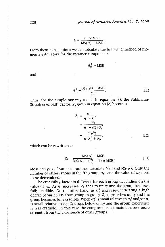
Thus, for the simple one-way model in equation (3), the Biihlmann­Straub credibility factor, Z, given in equation (2) becomes

(12)

which can be rewritten as

MS(lX) - MSE Zi = MS(lX) + (~~ - 1) x MSE'

(13)

Most analysis of variance routines calculate MSE and MS(lX). Only the number of observations in the ith group, ni , and the value of no need to be determined.

The credibility factor is different for each group depending on the value of ni. As ni increases, Zi goes to unity and the group becomes fully credible. On the other hand, as (Jl increases, indicating a high degree of variability from group to group, Zi approaches unity and the group becomes fully credible. When (Jl is small relative to (JJ and/or ni is small relative to no, Zi drops below unity and the group experience is less credible. In this case the compromise estimate borrows more strength from the experience of other groups.

Tolley, Nielsen, and Bachler: Credibility Calculations 229

Equation (13) provides a simple calculation of the credibility factor using output from ANOYA routines. Many times, however, the data have been summarized so that for each group i only the observed pure premium, say 17i., the number insured, ni, and the standard deviation, Si, are known. In this case the formulas can be used by first observing that

t - '" ni-Y .. =L.NYi..

i=l

(14)

Thus, MS(LX) is calculated as given in equation (9) using Y. as given in equation (14). Rearranging the terms in equation (9) yields a formula that is often easier to use. Explicitly,

MS(LX) = t ~ 1 (± ni17l- N17.~) 1=1

(15)

Second, MSE is calculated as in equation (8). The credibility factors Zi can be calculated using equation (13) where

the MSE is given by equation (8) and MS (LX) is calculated using equation (15) with 17 .. as defined in equation (14).

3 Calculation of Z via Computer Programs

3.1 Individual Data Case

To illustrate the formulas and computer programs we consider the hypothetical data given in Table 1. The data sets are small and would not be seriously considered as reliable insurance experience. With such small data sets, however, the details of calculations are more apparent. The data in Table 1 represent four hypothetical groups with claims for each group. We wish to determine the credibility factors for each group assuming that the four groups represent the entire experience of inter­est for the insurer.

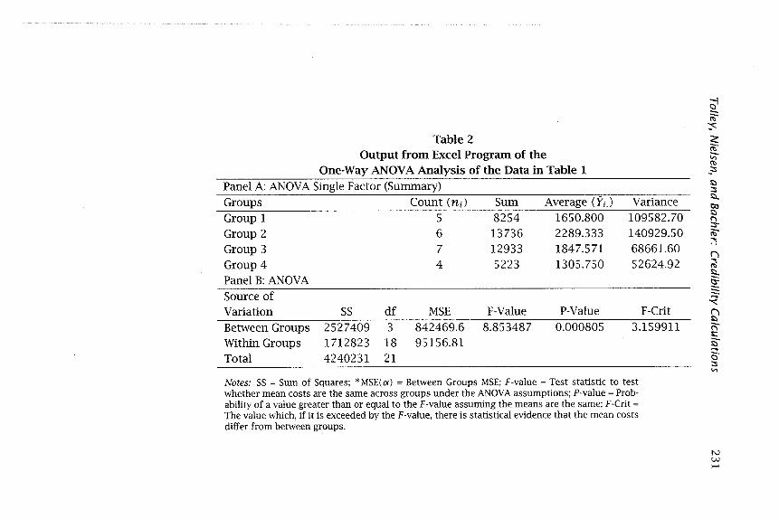
Table 2 gives the EXCEL 6 output for a one-way analysis of variance of the data in Table 1. To obtain this analysis we perform the following steps:

6EXCEL is a registered trademark of: Microsoft Corporation, One Microsoft Way, Redmond WA 98052-6399, USA.

230 Journal of Actuarial Practice, Vol. 7, 7999

Table 1 Hypothetical Individual Cost Data

For Four Groups of Insureds for a Single Year Groups

1 2 3 4 1550 1879 1440 1014 1325 2028 1601 1231 1417 2150 1790 1487 1824 2245 1852 1491 2138 2516 1998

2918 2081 2171

Step 1: Click the Data Analysis menu selection under Tools;

Step 2: We then click One-Way;

Step 3: As each column represents a different group, we indicate the Grouped by Columns option and then proceed.

The output consists of one table (Table 2) with two panels, Panel A and Panel B. The first column in Panel A lists the group name. The second gives the value of ni for group i, where i indicates the column of the group data. The fourth column gives Yi. for group i as given by equation (5). The fourth column of Panel B lists the MS(a) in the first row and the MSE in the second row.

Using the second column of Table 2, Panel A we calculate no using equation (10). For this equation t -1 = 4-1 = 3. The other components of the equation are given as:

N = 22

L ni = 126, and

no = (222 - 126)/(22 * 3) = 5.4242.

Table 2 Output from Excel Program of the

One-Way ANOV A Analysis of the Data in Table 1 Panel A: AN OVA Single Factor (Summary) Groups Count (ni) Sum Average (YiJ Variance Group 1 5 8254 1650.800 109582.70 Group 2 6 l3736 2289.333 140929.50 Group 3 7 12933 1847.571 68661.60 Group 4 4 5223 l305.750 52624.92 Panel B: ANOVA Source of Variation SS df MSE F-Value P-Value F-Crit Between Groups 2527409 3 842469.6 8.853487 0.000805 3.159911 Within Groups 1712823 18 95156.81 Total 4240231 21

Notes: SS = Sum of Squares; *MSE(()() = Between Groups MSE; F·value = Test statistic to test whether mean costs are the same across groups under the AN OVA assumptions; P-value = Prob­ability of a value greater than or equal to the F-value assuming the means are the same; F-Crit =

The value which, if it is exceeded by the F -value, there is statistical evidence that the mean costs differ from between groups.

Oi ~ :" <': ~.

<;:; n> ,::s t:l ::s tl.. OJ t:l ..., ::s­~ ~

~ tl..

~ ;;.

"" o r; s:: ~ .... o· ::s '"

N W >-'

232 Journal of Actuarial Practice, Vol. 7, 7999

Using these values we calculate the Zi for each group using equation (13). Explicitly, for group 1 we have

Z _ 842469.6 - 95156.81 1 - 842469.6 + ( - 1) x 95156.81

= 0.878631

Thus, the credibility score for group 1 is about 87.9 percent. Relative to the complete set of data available, the data on group 1 are relatively credible-there is little difference between the compromise estimate of the group pure premium and the estimate using the observed average of the group.

3.2 Grouped Data Case

Suppose that only the summary data consisting of ni, fl., and sf for each group are available (columns (2), (4), and (5) of Table 2, Panel A). In this case we can use equations (15) and (8) to calculate the components of equation (13). Explicitly we make the following calculations. First from equation (14) we have

Y. = (5 x 1650.8 + 6 x 2289.333 + 7 x 1847.571 + 4 x 1305.75)/22 40146

22 = 1824.818182.

Using these in. equation (15) we obtain

MS(()() = 75786559.41 - 73259150.73 3

2527408.68 3

= 842469.56

This is close to the value given in Table 2, Panel B (row (1), column (4)). The difference is due to roundoff error.

Calculation of MSE follows similarly using equation (8). Explicitly, we get

MSE = 1712822.66 18

= 95156.81

Tolley, Nielsen, and Bachler: Credibility Calculations 233

These results can be used to calculate the credibility scores as before. Computer code for the same calculations using SAS are given in the

appendix; no code is provided for SPSS. 7

4 Discussion

We have illustrated how the Buhlmann-Straub credibility factors can be calculated using one-way ANOVA statistical routines common in many computer programs. In order to form such scores the mean squares reported in the ANOV A tables must be used as given in equa­tion (13). Under certain situations estimated MS(lX) can be negative. In this case the value of Zi = 0 is used. This reduces the bias of the compromise estimate as shown by Morris (1983).

References

Buhlmann, H. "Experience Rating and Credibility." ASTIN Bulletin 4 (1967): 199-207.

Buhlmann, H. Mathematical Methods in Risk Theory. New York, N.Y.: Springer-Verlag, 1970.

Buhlmann, H. and Straub, E. "Glaubwlirdegkeit FUr Schadensatze." Mit­teilunger der Vereinigung Schweizerischer Versicherungsnathematiker 70 (1970): 111-133.

Dannenburg, D. "Cross Classification Credibility Models." Transactions of the 25th International Congress of Actuaries 4 (1995): 1-35.

Dannenburg, D.R., Kaas, R. and Goovaerts, M.l. Practical Actuarial Cred­ibility Models. Amsterdam, Holland: Institute of Actuarial Science and Econometrics, University of Amsterdam, 1996.

DeVylder, F. and Goovaerts, M. "Optimal Parameter Estimation Under Zero-Excess Assumptions in the Buhlmann-Straub Model." Insur­ance: Mathematics and Economics 11 (1992): 167-17l.

Ericson, W.A. "On the Posterior Mean and Variance of a Population Mean." Journal of the American Statistical Association 65 (1970): 649-652.

7SAS is a registered trademark of: SAS Institute Inc., Cary, NC 27512-8000, USA; and SPSS is a registered trademark of: SPSS Inc., 444 North Michigan Avenue, Chicago IL 60611, USA.

234 Journal of Actuarial Practice, Vol. 7, 1999

Goulet, V. "Principles and Applications of Credibility Theory." Journal of Actuarial Practice 6 (1998): 5-62.

Herzog, T.N. Credibility Theory. Winsted, Conn.: ACTEX Publications, 1996.

Hossack, LB., Pollard, J.H. and Zehnwirth, B. Introductory Statistics with Applications in General Insurance. Cambridge, England: Cambridge University Press, 1983.

Klugman, S. "Credibility for Classification Ratemaking via the Hierar­chical Normal Linear Model." Proceedings of the Casualty Actuarial Society 74 (1987): 272-32l.

Longley-Cook, L.H. "An Introduction to Credibility Theory." Proceedings of the Casualty Actuarial Society 49 (1962): 194-22l.

Morris, C and van Slyke, L. "Empirical Bayes Methods for Pricing Insur­ance Classes." Proceedings of the Business and Economics Statistics Section, American Statistical Association (1978): 579-582.

Morris, CN. "Parametric Emprical Bayes Inference: Theory and Appli­cations." Journal of the American Statistical Association 78 (1983): 47-65.

Mosteller, F. and Tukey, ].W. "Purposes of Analyzing Data That Come in a Form Inviting Us to Apply Tools From the Analysis of Variance." In Fundamentals of Exploratory Analysis of Variance. New York, N.Y.: John Wiley & Sons, 1991.

Neter, ]., Wasserman, W. and Craig, A.T. Applied Linear Statistical Mod­els. 3rd Edition. Boston, Mass.: Irwin, 1990.

Norberg, R. "The Credibility Approach to Ratemaking." Scandinavian ActuarialJournal (1979): 181-22l.

Philbrick, S.W. "An Examination of Credibility Concepts." Proceedings of the Casualty Actuarial Society 68 (1981): 195-219.

Rubin, D.B. "Using Empirical Bayes Techniques in the Law School Va­lidity Studies." Journal of the American Statistical Association 75 (1980): 801-827.

Scheffe, H. The Analysis of Variance. New York, N.Y.: John Wiley & Sons, 1959.

Tsutakawa, R.K. "Mixed Model for Analyzing Geographic Variability in Mortality Rates." Journal of the American Statistical Association 83 (1988): 37-42.

Venter, G.G. "Structured Credibility in Application-Hierarchical, Multi­dimensional and Multivariate Models." Actuarial Research Clearing

Tolley, Nielsen, and Bachler: Credibility Calculations 235

House (ARCH) 2 (1985): 267-308. (ARCH is a publication of the So­ciety of Actuaries, Schaumburg, Ill.)

Venter, G.G. "Credibility." In Foundations of Casualty Actuarial Science. Arlington, Va.: Casualty Actuarial Society, 1990.

Appendix

The codes for making credibility calculations using SAS for the data in Table 1 are given below. First we use the individual data. We have used the cards option. In practice one would read a data file. Below we give the code for grouped data. In both cases the amount of work to get the SAS code seems long relative to the simple problem considered. For longer, more practical problems, however, the benefits of SAS routines are more apparent.

DATA costs; IN FILE cards; INPUT cost group; CARDS;

1550 1 1325 1 1417 1 1824 1 2138 1 1879 2 2028 2 2150 2 2245 2 2516 2 2918 2 1440 3 1601 3 1790 3 1852 3 1998 3 2081 3 2171 3

236

1014 4 1231 4 1487 4 1491 4

RUN;

Journal of Actuarial Practice, Vol. 7, 7999

/*** Getting number of individuals per group ***/ PROC SQL;

CREATE TABLE counts AS SELECT DISTINCT group,count(group) AS number FROM costs GROUP BY group;

/*** Calculating n_not ***/ PROC SQL;

SELECT (sum(number)-(sum(number**2)/sum(number») /(count(number)-l)

INTO :n_not FROM counts;

/*** Calculating MSE, MSA ***/ PROC ANOVA DATA=costs OUTSTAT=results NOPRINT;

CLASS groL1P; MODEL cost=group;

RUN;

DATA _nulL; SET results; mean_sqr=ss/df; SELECT (_source_);

WHEN ("ERROR") CALL SYMPUTC"MSE",mean_sqr); WHEN ("GROUP") CALL SYMPUTC"MSA",mean_sqr);

END; RUN;

/*** Calculating credibilities ***/ DATA creds;

SET counts; cred=(&MSA-&MSE) / (&MSA+(&n_not/number-1) "'&MSE) ; KEEP group cred;

RUN;

Tolley, Nielsen, and Bachler: Credibility Calculations

PROC PRINT NOOBS DATA=creds; TITLE 'Credibility Factors for Individual Data';

RUN;

/****************** USING GROUPED DATA

******************/

DATA grouped; INFILE cards; INPUT group number avg_cost var_cost; CARDS;

1 58 1666 49597893 2 115 5051 216276545 3 81 4670 193990984 4 108 8966 757144094

RUN;

/*** Calculating n_not and the overall mean ***/ PROC SQL;

SELECT (sum(number)-(sum(number**2)/sum(number») /(count(number)-l), sum(avg_cost*number)/sum(number)

INTO :n_not, :y_bar2 FROM grouped;

/*** Calculating MSE, MSA ***/ PROC SQL;

SELECT 1/(count(group)-1)*(sum(number*avg_cost**2) -sum(number) >"&y_ba r2 >""(2) , 1/(sum(number)-count(group»*sum((number-1) ~'var _cost)

INTO :msa, :mse FROM grouped;

/*** Calculating credibilities ***/ DATA creds;

SET grouped; c red= (&msa-&mse) / (&msa+ (&n_not/numbe r-1) ~'&mse) ; KEEP group cred;

237

240 Journal of Actuarial Practice, Vol. 7, 1999

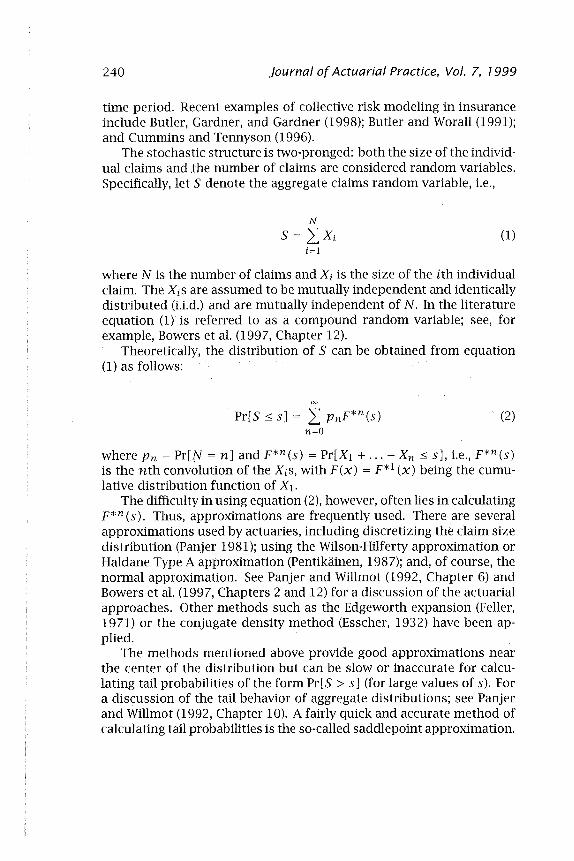
time period. Recent examples of collective risk modeling in insurance include Butler, Gardner, and Gardner (1998); Butler and Worall (991); and Cummins and Tennyson (996).

The stochastic structure is two-pronged: both the size of the individ­ual claims and .the number of claims are considered random variables. Specifically, let S denote the aggregate claims random variable, Le.,

(1)

where N is the number of claims and Xi is the size of the ith individual claim. The XiS are assumed to be mutually independent and identically distributed (LLd.) and are mutually independent of N. In the literature equation 0) is referred to as a compound random variable; see, for example, Bowers et al. (1997, Chapter 12).

Theoretically, the distribution of S can be obtained from equation (1) as follows:

00

Pr[S ::0; s] = I PnF*n(s) n=O

(2)

where Pn = Pr[jV = n] and F*n(s) = Pr[XI + ... + Xn ::0; s], Le., F*n(s) is the nth convolution of the XiS, with F(x) = F*l (x) being the cumu­lative distribution function of Xl.

The difficulty in using equation (2), however, often lies in calculating F*n (s). Thus, approximations are frequently used. There are several approximations used by actuaries, including discretizing the claim size distribution (Panjer 1981); using the Wilson-Hilferty approximation or Haldane Type A approximation (Pentikainen, 1987); and, of course, the normal approximation. See Panjer and Willmot (1992, Chapter 6) and Bowers et al. 0997, Chapters 2 and 12) for a discussion of the actuarial approaches. Other methods such as the Edgeworth expansion (Feller, 1971) or the conjugate density method (Esscher, 1932) have been ap­plied.

The methods mentioned above provide good approximations near the center of the distribution but can be slow or inaccurate for calcu­lating tail probabilities of the form Pr[S > s] (for large values of s). For a discussion of the tail behavior of aggregate distributions; see Panjer and Willmot (1992, Chapter 10). A fairly quick and accurate method of calculating tail probabilities is the so-called saddlepoint approximation.

Borowiak: Saddlepoint Approximation for Tail Probabilities 241

Since their introduction by Daniels (1954) saddlepoint approxima­tions have been utilized to approximate tail probabilities in a variety of situations; see, for example, Goutis and Casella (1999), Huzurbazar (1999), Butler and Sutton (1998), Tsuchiya and Konishi (1997), and Wood, Booth, and Butler (1993). Field and Ronchetti (1990) document the accuracy of these procedures for small sample sizes (even of sam­ple size one). In this paper a saddlepoint approximation is developed for Pr[S > s] and is applied to specific examples.

2 The Saddlepoint Approximation

The key assumption in the saddlepoint approximation is the as­sumption of the existence of the moment-generating functions corre­sponding to Xi and N, which are denoted by Mx(8) and MN(8), respec­tively, where e is a real valued parameter. 1 The moment-generating function of S, Ms(e), is then given by

Ms(8) = E[eos]

= E[E[eosIN]]

= MN(lOg(Mx (8)))· (3)

Equation (3) can be used to derive the well-known results on the mo­ments of compound sums of LLd. random variables:

Ils = E[S] = E[N]E[Xl] (4)

a-§ = Var[S] = Var[N](E[Xll)2 + E[N]Var[Xll. (5)

The saddlepoint approximation for the tail probability Pr[S > s] is adapted from Field and Ronchetti (1990) for sample size one. First let T denote the standardized random variable

S - Ils T=--

Us

lThe moment-generating function of a random variable Z is defined as

Mz(8) = E[eoz ], 8> O.

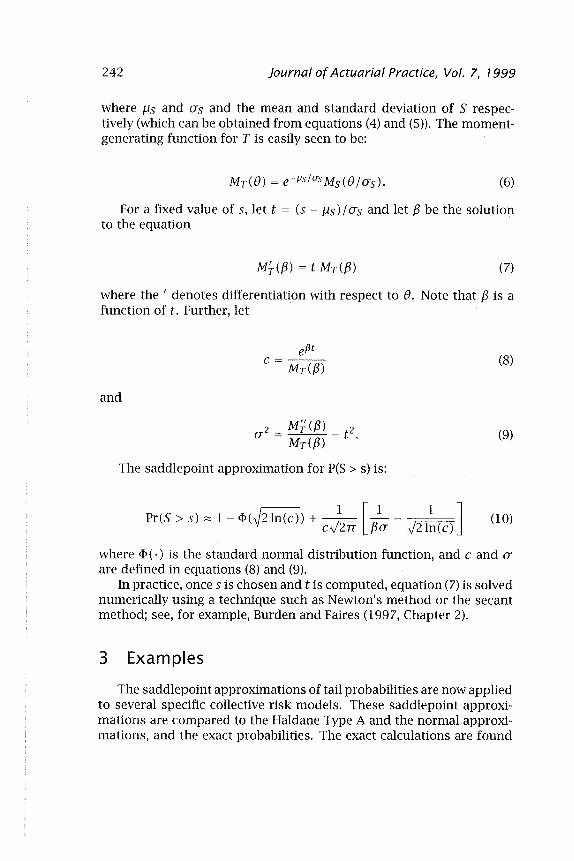
242 Journal of Actuarial Practice, Vol. 7, 1999

where J.1s and Us and the mean and standard deviation of S respec­tively (which can be obtained from equations (4) and (5)). The moment­generating function for T is easily seen to be:

(6)

For a fixed value of s, let t = (5 - J.1s) / Us and let [3 be the solution to the equation

M~([3) = t MT([3) (7)

where the I denotes differentiation with respect to e. Note that [3 is a function of t. Further, let

ef3 t

c = MT([3) (8)

and

2 _ My([3) _ t2 U - MT([3) . (9)

The saddlepoint approximation for P(S > s) is:

Pr(S > s) "" 1 - 4>(~21n(c)) + ~[_[31 - ~J (10) cv 2rr u 2In(c)

where 4>(.) is the standard normal distribution function, and c and u are defined in equations (8) and (9).

In practice, once 5 is chosen and t is computed, equation (7) is solved numerically using a technique such as Newton's method or the secant method; see, for example, Burden and Faires (1997, Chapter 2).

3 Examples

The saddlepoint approximations of tail probabilities are now applied to several specific collective risk models. These saddlepoint approxi­mations are compared to the Haldane Type A and the normal approxi­mations, and the exact probabilit'ies. The exact calculations are found

Borowiak: Saddlepoint Approximation for Tail Probabilities 243

by simulation using 10,000 repetitions, which gives accuracy to four decimal places.

If X has mean f.1x, standard deviation (J'x, and coefficient of skewness )'x, then the Haldane Type A approximation is as follows:

Pr[X ~ xo] "" <I> [( (1 + rxo)h - f.1(h, r)) / (J'(h, r)] (11)

where

- (xo - f.1x) x 0 = -'--"---'-"'-'-(J'x

(J'x r = - (12)

f.1x

h = 1 - )'x (l3) 3r 1 1

f.1(h, r) = 1 - 2"h(l - h)[l - 4(2 - h)(l - 3h)r2]r2 (14)

(J'(h,r)=hr~1-~(l-h)(l-3h)r2. (15)

The Haldane approximation is chosen because Pentikainen's (1987) re­sults show it to be, under certain circumstances, an accurate approxi­mation. Recall that the normal approximation is

Pr[X ~ xo] "" <I> [xo]. (16)

The relative errors shown in the tables are calculated as:

e atlve rror = . R I . E I Approximation Exact I Exact

3.1 Light and Medium Tailed Claim Size'Distributions

Example 1: Xl is normal random variables with mean f.1x = 100 and standard deviation (J'x = 10 while N is Poisson with mean i\ = 10. From equation (3)

244 Journal of Actuarial Practice, Vol. 7, 7999

Table 1 Approximating Tail Probabilities for

The Compound Normal-Poisson Model Relative Error

t [3 Exact Normal HALDA SADP 0.5 0.4637 0.2964 0.0411 0.0039 0.0034 1.0 0.8672 0.1575 0.0074 0.0077 0.0070 1.5 1.2243 0.0750 0.1089 0.0062 0.0087 2.0 1.5445 0.0303 0.2498 0.0125 0.0082 2.5 1.8347 0.0112 0.4469 0.0019 0.0089 3.0 2.1001 0.0036 0.6351 0.0091 0.0084

In this setting the central limit theorem is known to hold for large i\..

Example 2: Xl is a gamma random variable with a mean of Ilx = 100 and standard deviation CTx = 10. N is a negative binomial random variable with mean of ()( = 10 and and standard deviation}, = 20. Here

Ms(e) = [1 -q~; q [3)-0 r (18)

where q = 0.5, Ilx = [38, CTx = [3J8, ()( = rq/(I -q) and}' = rq/(l-q)2.

Table 2 Approximating Tail Probabilities for

The Compound Gamma-Negative Binomial Relative Error

t [3 Exact Normal HALDA SADP 0.5 0.4284 0.2684 0.1494 0.0961 0.0417 1.0 0.7502 0.1548 0.0252 0.0284 0.0032 1.5 1.001 0.0796 0.1608 0.0515 0.0050 2.0 1.203 0.0375 0.3920 0.6907 0.0027 2.5 1.369 0.0166 0.6265 0.3012 0.0084 3.0 1.508 0.0070 0.8086 0.4571 0.0100

Borowiak: Saddlepoint Approximation for Tail Probabilities 245

Example 3: Xl is an inverse Gaussian random variable with mean I1x = 100 and standard deviation (}x = 10. N is Poisson with mean i\ = 10. The moment-generating function for the inverse Gaussian distribution is

see Johnson and Kotz (1970, Chapter 15). Hence

Table 3 Approximating Tail Probabilities for

The Compound Inverse Gaussian-Poisson Model Relative Error

t f3 Exact Normal HALDA SADP 0.5 0.4537 0.2998 0.0290 0.0153 0.0147 l.0 0.8671 0.1629 0.0258 0.0258 0.0264 l.5 l.2242 0.0775 0.1381 0.0387 0.0413 2.0 l.5444 0.03 16 0.2785 0.0285 0.0348 2.5 1.8345 0.0119 0.4790 0.0588 0.0672 3.0 2.0998 0.0038 0.6474 0.0526 0.0526

These examples show that the saddlepoint approximation is supe­rior to the central limit theorem, but seems to be on par with the Hal­dane approximation in calculating tail probabilities. Next we consider a more difficult setting involving heavy tailed distributions.

4 Heavy Tailed Claim Size Distributions

The saddlepoint approximation requires the existence of the moment­generating function of the claim variable. For heavy tailed distributions, such as the Pareto (the moment-generating function does not exist)

246 Journal of Actuarial Practice, Vol. 7, 7999

and lognormal (the moment-generating function is not in convenient a closed form), an approximation is required. For these problem cases a censoring limit is imposed on the claim distribution.

For cases where the moment-generating function does not exist, the distribution of the claim variable is approximated utilizing an upper tail censoring limit. For small E the censoring limit, L, satisfies Pr[XI > L] = E. Let us define the censored claim random variable as

y. _ {Xi if Xi ::; L 1 - L if Xi> L.

The distribution function for the YiS is now

( ) _ {F(X) if x < L Fy x-I 'f L I X 2': •

The corresponding moment-generating function is

My(e) = J:=o eOXdF(x) + EeOL. (20)

The saddle point approximation is applied using the censoring moment­generating function in equation (20). This technique is now demon­strated on two examples of heavy tailed claim distributions. In both cases the number of claims is assumed to be Poisson with mean 5.

Example 4: Claims are assumed to follow a lognormal distributed with probability density function (pdf) of Xl is

2 !(X)=_l_ exp [_.!.(ln(X)-J.l)] -oo<x<oo. (21)

)2rr~ 2 ~

where J.l = 0 and ~ = 1. We assume that E = 0.001, which produces a censoring limit of L = 59.7697.

Example 5: Here we assume the claim size follows a Pareto distribution with distribution function given by

1 F(x) = 1- (1 +X)3'

Borowiak: Saddlepoint Approximation for Tail Probabilities 247

Table 4 Approximating Tail Probabilities for

The Compound Lognormal-Poisson Model Relative Error

t f3 Exact Normal HALDA SADP 0.5 0.7251 0.1628 0.8950 0.5565 0.0498 1.0 0.9501 0.0630 1.5190 1.3016 0.0825 1.5 1.0512 0.0241 1.7718 2.3361 0.0622 2.0 1.2001 0.0108 1.1111 1.0463 0.1574 2.5 1.4211 0.0047 0.3191 5.5319 0.3404

Again, E = 0.001, and this produces a censoring limit of L = 9.0. As in the previous section, normalized tail probabilities and the sad­

dlepoint approximations are compared to the exact values as obtained by simulation. These computations are listed in Tables 4 and 5.

Table 5 Approximating Tail Probabilities for

The Compound Pareto-Poisson Model Relative Error

t f3 Exact Normal HALDA SADP 0.5 0.6959 0.1664 0.8540 0.6280 0.03l3 1.0 0.9880 0.0688 1.3067 1.2456 0.1933 1.5 1.1623 0.0327 1.0428 1.5199 0.1804 2.0 1.2842 0.0165 0.3818 1.5091 0.0727 2.5 1.3772 0.0094 0.3404 1.1064 0.1596

For the heavy tailed distributions, the saddlepoint approximation is superior to the central limit theorem and the Haldane approximation in calculating' tail probabilities.

248 Journal of Actuarial Practice, Vol. 7, 7999

References

Bowers, N.L., Gerber, H.D., Hickman, J.c., Jones, DA and Nesbitt, c.]. Actuarial Mathematics, (2nd edition). Schaumburg, Ill.: Society of Actuaries, 1997.

Burden, R.L. and Faires, J.D. Numerical Analysis, (6th edition). New York, N.Y.: Brooks/Cole Publishing Company, 1997.

Butler, R.]., Gardner, H. and Gardner, H. (1998). "Workers Compensa­tion Costs When Maximum Benefits Change." journal of Risk and Uncertainty 15 (1998): 259-269.

Butler, R. and Sutton, R. "Saddlepoint Approximation for Multivariate Cumulative Distribution Functions and Probability Computations in Sampling Theory and Outlier Testing." journal of the American Sta­tistical Association 19, no. 442 (1998): 596-604.

Butler, R.J. and Worall, J.D. "Claim Reporting and Risk Bearing Moral Hazard in Workers Compensation." journal of Risk and Insurance 53 (1991): 191-204.

Cummins, J.D. and Tennyson, S. "Moral Hazard in Insurance Claiming: Evidence from Automobile Insurance." journal of Risk and Uncer­tainty 12 (1996): 29-50.

Daniels, H.E. "Saddlepoint Approximations in Statistics." Annals of Mathematical Statistics 25 (1954): 631-650.

Esscher, F. "On the Probability Function in Collective Risk Theory." Scan­dinavian Actuarial journal 15 (1932): 175-195.

Feller, W. An Introduction to Probability and Its Application, Volume 2, (2nd edition). New York, N.Y.: Wiley and Sons, 1971.

Field, C. and Ronchetti, E. Small Sample Asymptotics. IMS Lecture Notes­Monograph Series 13. Hayward, Calif.: Institute of Mathematical Statistics, 1990.

Goutis, C. and Casella, G. "Explaining the Saddlepoint Approximation." The American Statistician 53, no. 3 (1999): 216-224.

Huzurbazar, S. "Practical Saddlepoint Approximations." The American Statistician 53, no. 3 (1999): 225-232.

Johnson, N.L. and Kotz, S. Distributions in Statistics: Continuous Uni­variate Distributions, Volume 1. Boston, Mass.: Houghton Mifflin Company, 1970.

Panjer, H.H. "Recursive Evaluation of a Family of Compound Distribu­tions." ASTIN Bulletin 12 (1981): 22-26.

Borowiak: Saddlepoint Approximation for Tail Prohahilities 249

Panjer, H.H. and Willmot, G.E. Insurance Risk Models. Schaumburg, Ill.: Society of Actuaries, 1992.

Pentikiiinen, T. "Approximate Evaluation of the Distribution Function of Aggregate Claims." ASTIN Bulletin 17 (1987): 15-40.

Tsuchiya, T. and Konishi, S. "General Saddlepoint Approximation and Normalizing Transformations for Multivariate Statistics." Commu­nications in Statistics, Part A-Theory and Methods 26, no. 11 (1997): 2541-2563.

Wood, A.T., Booth, ].G. and Butler, R.W. "Saddlepoint Approximation to the CDF of Some Statistics with Nonnormal Limit Distributions." Journal of the American Statistical Association 88, no. 442 (1993): 680-686.