Credit and Business Cycles

Credit and Business Cycles

Christian Groth Emiliano Santoro

University of Copenhagen

December 2008

Groth & Santoro (Copenhagen) Credit and Business Cycles December 2008 1 / 49

Overview

Financial Hierarchy

Bank Lending Channel

Balance Sheet Channel

Credit Cycles


Overview Financial Hierarchy

Modigliani-Miller theorem (MM, 1958): �nancial structure isirrelevant to real outcomes

Perfect substitutability between di¤erent forms of funding

Cost of capital is the same regardless of the way funds are raised

This hypothesis is implicit in the IS-LM framework



MM theorem is based on the assumption of perfect and completeinformation

What�s at the root of imperfect substitutability?

Gap between internal �nance and total investmentAsymmetric information between lenders and borrowers

Asymmetric information or imperfect enforceability of �nancialcontracts:

Wedge between the cost of funds raised externally and the opportunitycost of internal funds: external �nance premium (EFP)EFP: cost implicit in the principal-agent problem characterizing therelationship between �nancial intermediaries and borrowers



Financial Hierarchy

The cost of di¤erent sources of external funding increases in thedegree of asymmetry between borrowers and lenders

Pecking order theory (or �nancial hierarchy): Myers and Majluf(Journal of Finance, 1984)

Firms prefer internal funds

If external �nance is required, �rms will resort to:1 debt �nance2 bonds3 equity �nance



Financial gap: �rms need to resort to the credit market

New equity issues are too costly due to adverse selection phenomena

At a given share price, only overvalued �rms are willing to sell theirshares

Potential shareholders anticipate that these companies are adverselyselected! no trade on the equity market

Under these conditions the announcement of an equity issue isgenerally interpreted as bad news by the investors

The stock market becomes a typical market for lemons (Akerlof,1970)



A sketch of the Financial Hierarchy theory

Internal �nance (A): retained pro�ts (cash �ow tout-court) which inturn constitute the net worth

The cost of internal �nance can be quanti�ed based on the concept ofopportunity cost (OC)

The OC of internal �nance equals the interest rate on a �nancialinvestment the �rm could undertake and that it must renounce if thereal investment is entirely covered with internal �nance (r)



Demand for capital K = f (c) f0< 0

This can be derived from a pro�t maximization problem

In this case investment takes place up to the point where

MCK = MPK



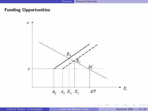
Funding Opportunities



In a MM world, external and internal �nance would have the samecost (r).

Thus c = r

The ith �rm would invest up to KM

The gap KM � A0 is covered with external �nance and leverageequals:

KM � A0KM

= 1� a0



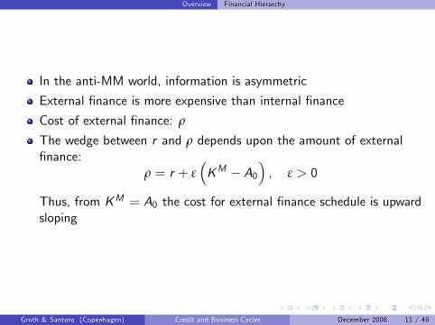
In the anti-MM world, information is asymmetric

External �nance is more expensive than internal �nance

Cost of external �nance: ρ

The wedge between r and ρ depends upon the amount of external�nance:

ρ = r + ε�KM � A0

�, ε > 0

Thus, from KM = A0 the cost for external �nance schedule is upwardsloping



Conclusions

Ine¢ cient exploitation of resources

Relevance of �nancial structure, compared to the MM paradigm:

Assume net worth increases from A0 to A1


Overview The Credit View of the Transmission Mechanism

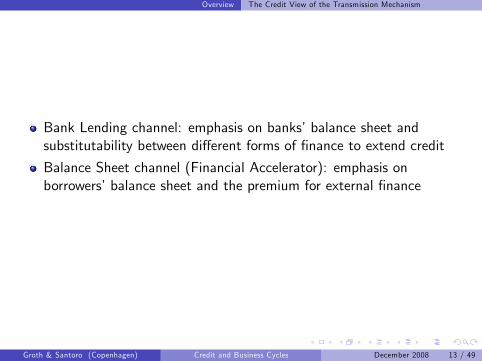
Bank Lending channel: emphasis on banks�balance sheet andsubstitutability between di¤erent forms of �nance to extend credit

Balance Sheet channel (Financial Accelerator): emphasis onborrowers�balance sheet and the premium for external �nance


Overview The Credit View of the Transmission Mechanism

Some Literature

Bank Lending view: Bernanke and Blinder (AER, 1988)

Balance Sheet channel: Greenwald and Stiglitz (QJE, 1993),Bernanke and Gertler (AER, 1989) and Kiyotaki and Moore (JPE,1997)

These frameworks emphasize the role �nancial frictions and theinteraction of heterogeneous agents

Renewed interest for the Wicksellian view that credit has bothrelevance in the propagation of business cycles and MPTM

Distinct role played by �nancial assets and liabilities and the need todistinguish between di¤erent types of non-monetary assets


Overview The Bank Lending Channel

The bank lending channel highlights the nature of credit and thespecial role played by commercial banks in the credit markets

Essence of the mechanism: monetary policy can a¤ect the external�nancial premium by in�uencing the supply of intermediated credit

Model economy: commercial banks represent the only source ofexternal funding

Banks�liabilities: deposits

Balance sheet:

ASSETS LIABILITIESReserves (r) Deposits (D)Loans (D � r)


Overview The Bank Lending Channel

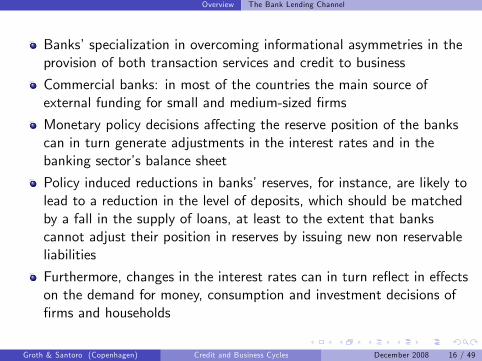
Banks�specialization in overcoming informational asymmetries in theprovision of both transaction services and credit to business

Commercial banks: in most of the countries the main source ofexternal funding for small and medium-sized �rms

Monetary policy decisions a¤ecting the reserve position of the bankscan in turn generate adjustments in the interest rates and in thebanking sector�s balance sheet

Policy induced reductions in banks�reserves, for instance, are likely tolead to a reduction in the level of deposits, which should be matchedby a fall in the supply of loans, at least to the extent that bankscannot adjust their position in reserves by issuing new non reservableliabilities

Furthermore, changes in the interest rates can in turn re�ect in e¤ectson the demand for money, consumption and investment decisions of�rms and households


Overview Credit Cycles: Kiyotaki and Moore (JPE, 1997)

Kiyotaki and Moore (1997) (KM hereafter)

Asymmetric information between borrowers and lenders

Moral hazard: lenders face a maximum limit to the credit they canobtain

Role of collateralizable assets

Collateral constraints a¤ect the scale of production: underutilizationof resources

The higher the collateral value, the higher the credit obtained and inturn investment spending and production



The economy is composed by a large number long-lived agents: 2categories

Farmers: �nancially constrained agents who produce by means ofinalienable human capital

Gatherers: agents endowed with alienable human capital, and hence�nancially unconstrained

The distribution of the agents according to their nature isexogenously postulated by KM

Two goods:

fruit (output)land: a durable and collateralizable good, whose supply is exogenouslyimposed to K



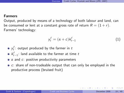
FarmersOutput, produced by means of a technology of both labour and land, canbe consumed or lent at a constant gross rate of return R = (1+ r).Farmers�technology:

y ft = (α+ c)kft�1 (1)

y ft : output produced by the farmer in t

k ft�1: land available to the farmer at time t

α and c : positive productivity parameters

c : share of non-tradeable output that can only be employed in theproductive process (bruised fruit)



GatherersGatherers access to the following technology:

ygt = f (kgt�1) (2)

ygt : output of the gatherer in t

f (�): decreasing returns to scale technologykgt�1: land available to the gatherer at time t � 1Production process: time-to-build technology



Inalienability and Impatience

Each farmer�s technology is individual-speci�c

Once the production has started, no one can successfully completethe productive process but the farmer

In principle, farmers have incentive to threaten their creditors towithdraw their labour and default

KM assume that lenders cannot force borrowers to repay their debtsunless previously secured

β < β0: heterogeneity is characterized by di¤erent discount rates

across households

Furthermore, if discount rates are equal then the steady state incomedistribution would be indeterminate: a number of hypothesis arenecessary



Collateral ConstraintGatherers collateralize farmers�land, by imposing the following constraint:

bft =qt+1k ftR

(3)

bft : loanqt+1: price of the land at time t + 1.Flow-of-funds constraint

y ft + bft = qt∆k

ft + Rb

ft�1 + c

ft (4)

c ft : farmers�consumption



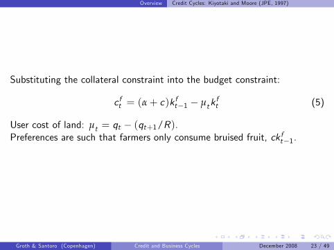
Substituting the collateral constraint into the budget constraint:

c ft = (α+ c)kft�1 � µtk

ft (5)

User cost of land: µt = qt � (qt+1/R).Preferences are such that farmers only consume bruised fruit, ck ft�1.



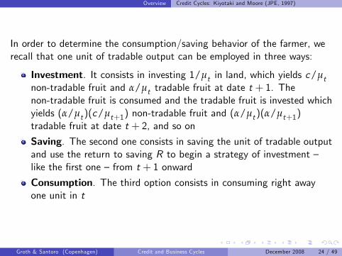
In order to determine the consumption/saving behavior of the farmer, werecall that one unit of tradable output can be employed in three ways:

Investment. It consists in investing 1/µt in land, which yields c/µtnon-tradable fruit and α/µt tradable fruit at date t + 1. Thenon-tradable fruit is consumed and the tradable fruit is invested whichyields (α/µt)(c/µt+1) non-tradable fruit and (α/µt)(α/µt+1)tradable fruit at date t + 2, and so on

Saving. The second one consists in saving the unit of tradable outputand use the return to saving R to begin a strategy of investment �like the �rst one � from t + 1 onward

Consumption. The third option consists in consuming right awayone unit in t



Alternative paths:

Inv. : 0,cµt,

α

µt

cµt+1

,α

µt

α

µt+1

cµt+2

, ....

Sav. : 0, 0,Rc

µt+1,R

α

µt+1

cµt+2

, ....

Cons. : 1, 0, 0, ....

Steady state:

Inv.: 0,cµ,

α

µ

cµ,

α

µ

α

µ

cµ, ....

Sav. : 0, 0,Rcµ,R

α

µ

cµ, ....

Cons. : 1, 0, 0, ....



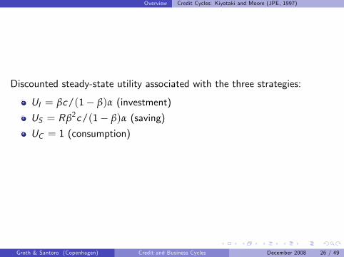
Discounted steady-state utility associated with the three strategies:

UI = βc/(1� β)α (investment)

US = Rβ2c/(1� β)α (saving)

UC = 1 (consumption)



Need to impose a condition in order to ensure that farmers will actuallyinvest, rather than saving/consuming:

UI > USUI > UC

Assumption 1Using the fact that

UI > US

entrepreneurs eat all their non-tradable output i¤:

1β> R =

1

β0 .



Assumption 2Farmers consume no more than the bruised fruit and use all tradableoutput for making deposits:

UI > UC

which in turn translates into

c >�1β� 1

�α.



Farmer�s demand for land is given by

k ft =1µt[(α+ qt )k ft�1 � Rbft�1] =

α

µtk ft�1 (6)

Substituting this expression in the collateral condition:

bft =qt+1αk ft�1Rµt

(7)



Alienability of human capital for the gatherers implies the existence of asingle constraint:

ygt + Rbgt�1 = qt∆k

gt + b

gt + c

gt (8)

As k ft = K � kgt :cgt = f (k

gt�1) + µt (K � k

gt ) (9)

The maximization problem for the gatherer implies that his preferences aresuch that Rµt = f

0(kgt ). Demand for land:

kgt = f0�1(Rµt ) (10)



For a given level of farmers�landholding and debt at the previous date anequilibrium from date t onward is characterized by the path:

f (qt+s ,Kt+s ,Bt+s )j s � 0g

This satis�es �ow-of-funds constr., coll. constr. and Euler equation of thegatherer.Rule out bubbles (transversality condition):

lims!∞

n�β0�sqt+s

o= 0



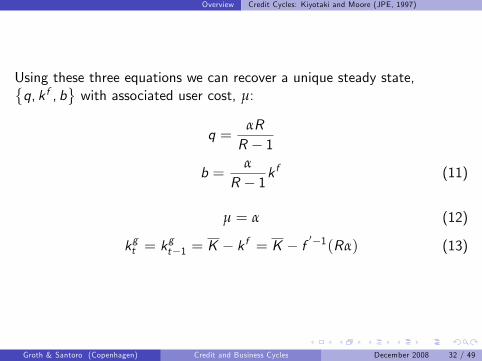
Using these three equations we can recover a unique steady state,�q, k f , b

with associated user cost, µ:

q =αRR � 1

b =α

R � 1kf (11)

µ = α (12)

kgt = kgt�1 = K � k f = K � f

0�1(Rα) (13)





We log-linearize the model economy around the steady state:

� bk ftbqt�=

"η1+η 0

�R�1η R

# � bk ft�1bqt�1�

η : elasticity of the residual supply of farmers�land with respect tothe user cost at the steady state:

1η=d log µ

�k ft�

d log k ft

��k ft =k f

= � d log f0(kgt )

d log kgt

��k gt =K�k f

� k f

K � k f

We consider f 00(�) < 0 to ensure that η is positive

Jacobian Matrix: lower triangular



Productivity Shock

At time t � 1, we assume the model economy is at the steady stateWe introduce an unexpected one-period shock to farmers�productivity, denoted by ∆.From time tand t + 1 the production technologies of the two agentsreturn to their equilibrium level

Perfect foresight: the shock is known to be temporary



Let us consider the BC of the farmer:

µtkft = [(α+ qt )k

ft�1 � Rbft�1]

Log-linear approximation around the steady state:

RHS ! [α+ ∆α+ qt � q]k f ! [α+ ∆α+ qbqt ]k fLHS !

�1+

�1+

1η

�� bk ftAfter time t the system returns to its original position

The �nancial constraint faced by the farmer holds with equality(β < β

0)



Percentage deviation of land from its steady state:

bk ft = ηR(R � 1) (η + 1)bqt + η∆

η + 1, (14)

From time t + 1 onwards, land dynamics will turn on the following path:

bk ft+s = � η

1+ η

�s bk ft , s > 0 (15)

Next, we need to determine the evolution of the asset price, qt . From theGatherer�s Euler equation:

qt = β0f 0�K � k ft

�+ β

0qt+1 (16)



After log-linearizing the Euler condition and plug it back into the linearizedconstraint of the farmer:

bqt = (R � 1) (η + 1)η ((η + 1)R � η)

bk ft (17)

We solve the resulting system to obtain:

bqt =∆η, (18)

bk ft =η

1+ η

0BB@1+ 1η

RR � 1| {z }

Ampli�cation Factor

1CCA∆. (19)



The role of elasticity ηPersistence:

bk ft+s = � η

1+ η

�s bk ft , s > 0

Market Clearing: �1+

1η

�bk ft = ∆+R

R � 1bqt



Extended Version: Section II KM (1997)

Let us assume that there is a continuum of farmers, as in the originalKM framework

Land as a reproducible asset

Depreciation

Probability of investing

A fraction π of farmers can invest (entrepreneurs), while 1� πcannot (households)



EntrepreneursFlow-of-funds Constraint

y fi ,t + bfi ,t = qt

�k fi ,t � k fi ,t�1

�+ φ

�k fi ,t � λk fi ,t�1

�+ Rbfi ,t�1 + c

fi ,t (20)

φ�k fi ,t � λk fi ,t

�: input for reproduction of capital

Collateral Constraint

bfi ,t =qt+1k fi ,tR

Assuming that investing is strictly better than consuming, the ith

entrepreneur faces the following constraint:�qt + φ� qt+1

R

�k fi ,t = (α+ λφ+ qt ) k fi ,t�1 � Rbfi ,t�1



Households

k fj ,t = λk fj ,t�1

In this case, land is solely subject to depreciation



AggregationLand Dynamics

Kt =Zk fj ,tdj +

Zk fi ,tdi =

= (1� π) λKt�1 +π�

qt + φ� qt+1R

� [(α+ λφ+ qt )Kt�1 � RBt�1]

Debt Dynamics

Bt = qt (Kt �Kt�1) + φ (Kt � λKt�1) + RBt�1

Asset Price (Gatherer�s Euler Equation)

R =f0 �K �Kt

�+ qt+1

qt



Numerical example

0 10 20 30 40 50 60 70 80 900.05

0

0.05

0.1

0.15qt

time

0 10 20 30 40 50 60 70 80 900.1

0

0.1

0.2

0.3

Kt D

t

time



Numerical Simulations (π = 0.5)

0 10 20 30 40 50 60 70 80 900

0.05

0.1

0.15

0.2qt

time

0 10 20 30 40 50 60 70 80 900

0.2

0.4

0.6

0.8

Kt D

t

time



Numerical Simulations (π = 0.8)

0 10 20 30 40 50 60 70 80 900

0.05

0.1

0.15

0.2qt

time

0 10 20 30 40 50 60 70 80 900

0.2

0.4

0.6

0.8

Kt D

t

time


Overview The Role of Capital Requirements

Loan-to-value (LTV) ratio: amount of the loan as a percentage of thetotal appraised value of real property:

bfi ,t = χqt+1k fi ,tR

0 < χ � 1

χ : LTVAs χ ", the quali�cation guidelines for certain mortgage programsbecome more strict

Lenders can require borrowers of high LTV loans to buy mortgageinsurance



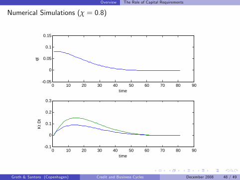
Numerical Simulations (χ = 0.8)

0 10 20 30 40 50 60 70 80 900.05

0

0.05

0.1

0.15qt

time

0 10 20 30 40 50 60 70 80 900.1

0

0.1

0.2

0.3

Kt D

t

time



Numerical Simulations (χ = 0.5)

0 50 100 150 200 2500

0.01

0.02

0.03

0.04qt

time

0 50 100 150 200 2500

0.02

0.04

0.06

0.08

Kt D

t

time


Date post:	15-Jan-2022
Category:	Documents
Upload:	others
View:	2 times
Download:	0 times

Credit and Business Cycles

Documents