Credit Crunch, Flight to Quality and Evergreening: An Analysis

Credit Crunch, Flight to Quality andEvergreening: An Analysis of Bank-Firm

Relationships After Lehman �

Ugo Albertazzi and Domenico J. MarchettiBanca d�Italia

Abstract

This paper analyzes the e¤ects of the �nancial crisis on credit sup-ply by using highly detailed data on bank-�rm relationships in Italyafter Lehman�s collapse. We control for �rms�unobservable character-istics, such as credit demand and borrower risk, by exploiting multiplelending. We �nd evidence of a contraction of credit supply, associ-ated with low bank capitalization and scarce liquidity. The ability ofborrowers to compensate through substitution across banks appearsto have been limited. We also document that larger low-capitalizedbanks reallocated loans away from riskier �rms, contributing to creditprociclicality. Such a ��ight to quality�has not occurred for smallerlow-capitalized banks. We argue that, among other things, this mayhave re�ected evergreening practices. We provide corroborating evi-dence based on data on borrowers�productivity and interest rates atbank-�rm level.

�The views in this paper are those of the authors only and do not necessarily re�ectthose of the Bank of Italy. Helpful comments were received from Paolo Angelini, MatteoBugamelli, Riccardo De Bonis, Eugenio Gaiotti, Simon Gilchrist, Luigi Guiso, GiorgioGobbi, Francesca Lotti, Paolo Mistrulli, Fabio Panetta, Diego Rodriguez de la Palenzuela,Carmelo Salleo, Fabiano Schivardi, Alessandro Secchi, Enrico Sette and seminar partici-pants at Bank of Italy, EIEF, University of Bologna, the 2009 NBER Summer Institute,the 2009 CEPR-Bank of Finland-CBS conference on �Credit crunch and the macroecon-omy�and the 2010 CEPR-Tilburg conference on �Procyclicality and �nancial regulation�.Responsability for any error is entirely our own. E-mail: [email protected];[email protected].

1

Keywords: crunch; bank capital; �ight to quality; evergreening.JEL codes: E44, E51, G21, G34, L16.

1 Introduction

Since the start of the recent �nancial crisis there has been an intense debateon whether a credit crunch was taking place, broadly de�ned as a situationwhere banks become abnormally reluctant to grant loans to the economy,especially to �rms. The debate has attracted not only economists but alsopoliticians and the public at large, for its important implications. A con-traction of credit supply is likely to be particularly harmful during a periodof weak economic activity as �rms�liquidity bu¤ers are low and a dramaticcutback in their investment spending may exacerbate the dampening e¤ectsof the recession on production and employment.One important factor which may lead to a contraction in credit supply is

related to the di¢ culties that banks encounter on the liability side of theirbalance sheets and, above all, in maintaining an adequate level of capital,whether in connection with prudential regulation or market discipline.1 Wor-ries intensi�ed after the collapse of Lehman Brothers when credit growth felldramatically in all the developed economies.However, despite the intense debate and the massive interventions by

public authorities, conclusive evidence of the existence of a credit crunch isstill not available.2 In particular, the need for e¤ective control of develop-ments in credit demand makes the identi�cation of changes in credit supplyquite di¢ cult (e.g., Udell, 2009).An additional factor is that banks�willingness to lend to a given �rm may

diminish because of an increase in perceived risk and for other good reasons.Basic corporate �nance principles suggest that some rationing in �nancialmarkets arises as a second best device to face incentive issues: as entrepre-neurs should maintain a su¢ cient stake in the returns on the investment,their debt capacity is limited by their own resources. Disentangling thesesources of supply contraction from that associated with capital constraintsis di¢ cult, as typically they all get exacerbated during crises.

1This is why the label �capital crunch�was initially introduced (see Bernanke et al.,1991).

2At an earlier stage of the crisis, when credit growth was deacreasing but still robust,some disputed the very existence of a credit crunch (Chari et al., 2008).

2

Previous studies have tried to overcome these di¢ culties in several waysbut, due to data limitation, could not properly control for loan demand.Peek and Rosengren (1995), using US bank-level data, document a strongercontraction of credit by undercapitalized banks during the 1990-91 reces-sion. Although highly suggestive, this evidence is not fully persuasive giventhat di¤erences in bank capital are likely to be associated with di¤erencesin borrowers� quality, so that di¤erences in credit growth may simply re-�ect di¤erences in �rms�conditions rather than in banks�conditions. Morestructural evidence with bank-level data is supplied by Peek and Rosengren(2000), who show that losses in Japan prompted US subsidiaries of Japanesebanks to cut back credit in the United States. Woo (2003), based on Japanesedata, documents a stronger contraction of credit by undercapitalized banksin 1997, when the indulgence towards banks of government and regulatorsceased. A similar approach, based on information on loan rejection rates overthe current �nancial crisis, is followed by Puri, Rocholl and Ste¤en (2009),who �nd that German saving banks a¢ liated with Landesbanken heavilyexposed to subprime lending reduced their acceptance rates by more thanother saving banks.3

In this work we provide robust evidence of a credit crunch, by using highlydetailed data on bank-�rm relationships after Lehman�s collapse, based ona representative sample of Italian �rms. The main feature of our empir-ical analysis is that we control for �rm�s speci�c risk and credit demandby exploiting the widespread use in Italy of multiple lenders (Detragiacheet al., 2000), which allows us to use �xed e¤ects capturing all �rms� un-observable characteristics.4 ;5 The period analyzed is the six-month period

3Other papers try to exploit �rm or sectoral level data, but cannot distinguish �pure�from other supply factors. Dell�Ariccia et al. (2008) identify loan supply factors by exploit-ing sectoral di¤erences in dependence on the banking sector; Borensztein and Lee (2002)have used information at the �rm level and proxied credit demand with some observ-able balance sheet items (e.g., net investment and cash-�ow). Perhaps most convincingly,Jiménez et al. (2009) go one step further by analyzing individual bank-�rm relationshipsin Spain until December 2008; they show that undercapitalized banks were more likely toreject a given borrower�s loan application.

4This is di¤erent from having �rm-speci�c �xed e¤ects in a standard panel set-upwith repeated cross sections, since in that environment �xed e¤ects would capture all timeinvariant unobservable features which clearly cannot include (time varying) credit demand.

5Unlike Jiménez et al. (2009), who also consider individual bank-�rm relationships,we look at credit dynamics rather than loan rejections. There are many reasons whyloan rejection rates may not re�ect only lending policies. For instance, if there is a cost

3

after Lehman�s failure (September 2008-March 2009), when the �nancial cri-sis erupted and credit growth collapsed dramatically everywhere (in Italy the3-month growth of credit to �rms fell from 8% to 1%, on a annualized basis;the dynamics of loans has stagnated since then, in Italy as in the rest of theeuro area and the other major economies; see Figure 1). This is also when,according to evidence based on bank survey data, credit supply e¤ects weremost pronounced.6

In the investigation of the credit crunch, Italy is an interesting case tostudy for two main reasons. It is a bank-based economy, so that distortions incredit supply may have a sizable impact;7 more generally, because of commoneconomic and banking features, the analysis of credit developments in Italycan help to shed light on developments in the rest of continental Europe.Moreover, because of the data requirements of banking supervision, a uniquedataset is available for the Italian economy, which includes timely informationon outstanding loans at bank-�rm level.We also investigate whether the (capital) credit crunch had a diversi�ed

impact across �rms, in particular according to borrower risk. There are sev-eral reasons why this may be so. For instance, the higher risk-sensitivenessof the Basle II capital requirements may induce a bias toward less risky bor-rowers. Other mechanisms, such as evergreening, may work in the oppositedirection. According to the latter notion (also known as forbearance lending,unnatural selection or zombie lending), under-capitalized banks may delaythe recognition of losses on their credit portfolio by ine¢ ciently rolling overloans to otherwise insolvent borrowers, in order not to cause a further im-pairment of their reported capital and pro�tability (Peek and Rosengren,2005).Unnatural selection in credit allocation has been largely documented with

regard to the long-lasting Japanese stagnation of the 1990s, to which it con-tributed in several ways (Caballero et al., 2008). Several observers haveemphasized the similarities with the current �nancial crisis (e.g., Hoshi and

associated with the decision to apply for a loan, then the expectation of a tighter (looser)lending policy may discourage (encourage) applicants (one obvious cost is related to thepossibility that a bank may get some information on previous rejections from the otherlenders, as happens in Italy).

6See Del Giovane et al. (2010).7At the end of 2008, the ratio of total bank credit to nominal GDP amounted to 60%

in the United States, compared to 112% in Italy (140% in the euro area as a whole, higherthan in Italy mainly because of the low level of Italian households�indebtedness).

4

Kashyap, 2008; Kobayashi, 2008). It is therefore natural to ask if those creditmarket ine¢ ciencies could take place in other economies beyond the Japaneseone. Indeed, the introduction in 2008 of Basle II standards, with their moreprocyclical capital requirements, may have contributed worldwide to the in-creasing di¢ culties faced by troubled banks in maintaining an adequate levelof capitalization.8

We �nd substantial di¤erences across lenders in the nexus between poorbank capitalization and the attitude towards borrower�s risk. In particu-lar, we show that larger low-capitalized banks reallocated loans away fromriskier borrowers. Such ��ight to quality�has not occurred for smaller low-capitalized banks. This �nding is consistent with evergreening but also withother explanations (for example, with smaller banks being less a¤ected byBasle II risk-sensitive capital requirements). We provide evidence that sug-gests evergreening did play a role by using data on borrowers�productivityand interest rates at bank-�rm level.Our contribution to the literature is threefold. We provide robust ev-

idence of a bank capital credit crunch. As to evergreening, our analysisrepresents the �rst attempt to our knowledge to study this issue beyond thecase of Japan. Furthermore, this paper brings an improvement in the wayimpaired borrowers are identi�ed. While previous contributions have mainlyfocused on balance sheet indicators of borrowers�quality, we also considerinformation on �rm�s economic fundamentals and competitiveness (based onTFP measures). Crucially, this allows us to disentangle ine¢ cient lendingpatterns such as evergreening from the opposite phenomenon of �patience�(namely the extension of credit to economically sound �rms which undergotemporary �nancial di¢ culties and appear risky). Altogether, we show thatan excessive generalized credit tightening and the extension of �cheap�creditto selected (risky) borrowers may well coexist, both induced by low bankcapitalization.9

The remainder of the paper is organized as follows. The next sectionpresents a simple model where capital constraints are introduced into a stan-dard model of borrowing capacity. Section 3 describes the data. Section 4presents the main evidence of a bank capital credit crunch. Section 5 ana-lyzes the heterogeneity of the crunch across �rms and banks, in particular

8See e.g. Panetta et al. (2009).9It has already been shown for transition economies that credit crunch and soft budget

constraint are not mutually exclusive (Berglöf and Roland, 1997).

5

with respect to borrower risk. Section 6 investigates the role of relationshiplending. Finally, Section 7 draws some conclusions.

2 The Analytical Framework

In this section we slightly extend a basic corporate �nance model of bor-rowing capacity in order to illustrate the theoretical underpinnings of ourempirical analysis. We show how our estimations can identify two interre-lated but distinct mechanisms, namely a bank capital crunch and e¢ cientcredit rationing.Let�s consider an economy populated by N entrepreneurs, indexed by i,

each endowed with a risky investment project. The expected return dependson the behavior of the entrepreneur which is not negotiable. The investmentis pro�table only if the entrepreneur behaves correctly (for example by ex-erting adequate e¤ort); should he misbehave, he would enjoy some privatebene�ts. Each entrepreneur is endowed with an amount of cash (or equity)equal to Ai.10

If the total investment required by the project, Ii, is larger than Ai, theentrepreneur can borrow the di¤erence (Ii � Ai) from a bank.As the behavior of the entrepreneur cannot be determined by contractual

provisions, he will choose an adequate level of e¤ort in equilibrium only if it isadvantageous for him to do so (in other words, if the incentive compatibilityconstraint is satis�ed). A standard result is that, for this to be the case,the borrower should keep a su¢ cient stake in the returns on the investment;more precisely, under quite general conditions it can be shown that thereexists a multiplier ki>1 such that Ii in equilibrium is equal to:

I 0i = min(Aiki; I�i ) (1)

where I�i is the optimal level of investment (the �rst-best solution, whereall agency frictions are ruled out by assumption). With some approximation,I�i can be thought of as loan demand.The intuition is that, whenever I�i >Aiki, there is some rationing (I

�i � Aiki),

and its extent is related to the severity of the agency costs (ki is a decreasing

10More generally, Ai can be interpreted as a measure of balance sheet conditions; a highAi characterizes a �rm with a relatively small debt or relatively high levels of cash, equityor �xed capital which can be used as collateral.

6

function of the private bene�ts that the entrepreneur enjoys by misbehav-ing).11

Let�s consider now the presence of a (binding) capital constraint. Ex-cluding by assumption the uninteresting case where I�i < Ai, the capitalconstraint can be written as:

NXi=1

(Ii � Ai) � C (2)

where C, bank capital, and are positive and exogenously given (the lefthand side is total lending by the bank). This constraint can be interpretedas representing either the prudential capital regulation ( = 1=0:08) or moregenerally the market discipline which limits the bank�s access to �nancialmarkets (for the same reasons as outlined above for a generic �rm). Thesolution is readily obtained by assuming so-called type I rationing, namelythat lending to each individual borrower is reduced proportionally to thelevel such that constraint (2) is satis�ed with an equality.12 With this sim-plifying hypothesis, lending to �rm i, denoted as L00i to distinguish it fromthe unconstrained level L0i, is equal to:

L00i = L0i ( C=L

0) = Ai (ki � 1) ( C=L0) (3)

with L0 =P

i=1;:::;N L0i. Two remarks are in order. First, since L

00i < L

0i,

the total rationing imposed on a �rm is larger when capital constraints arebinding. This additional source of rationing is exactly what the empiricalanalysis reported in Section 5 seeks to measure. The welfare implications ofthe two types of rationing are quite di¤erent. If banks granted more creditthan L0i, they would determine a misalignment of �rms�incentives; on thecontrary, if banks granted more credit than L00i then �rm�s incentives wouldstill be preserved.The two sources of rationing are likely to move together: when business

activity slows down, �rms are likely to undergo an erosion of equity andpossibly face harsher agency frictions, implying a lower L0i; similarly, therationing brought by the erosion of bank equity, i.e. the bank capital crunch,is likely to increase during recessions, when banks tend to su¤er higher creditlosses.11For more details on the notion of equity multiplier see, for example, Tirole (2006).12The opposite case of type II rationing � i.e., some borrowers within a homogeneous

group receive credit while others do not � is discussed below.

7

The rationale of our empirical strategy is suggested by the simple com-parison of the two solutions L0i and L

00i . With no shortage of bank capital,

lending to a given �rm simply re�ects its characteristics, such as its equityAi and agency costs ki. In the alternative case where C <

PNi=1Ai (ki � 1),

lending to a �rm is also in�uenced by the lender�s characteristics, in partic-ular its capitalization C. Taking logs of (3) leads to the regression equation:

ln (Li;j) = �0 + �1 ln (Ai (ki � 1)) + �2 ln (Cj) + "i;j (4)

where �0 = ln� =�P

i=1;:::;N Ai (ki � 1)��

and "i;j is an error term. Thenotation Li;j stands for loans extended to �rm i by bank j. The null hypoth-esis of no credit crunch is H0 : �2 = 0, against the alternative H1 : �2 > 0.By introducing the index j for banks we implicitly dropped the assump-

tion of the existence of a unique bank; this is done not only for the sake ofrealism, but also for in order to introduce an important methodological fea-ture of our analysis. In principle, estimating (4) requires detailed informationnot just on balance sheet items Ai but also on variables, such as the agencycosts ki, which are hardly observable. Notwithstanding, supposing that thereis availability of information on loan dynamics at bank-�rm level, an unbi-ased estimation of the coe¢ cient �2 can be obtained by using �rm-level �xede¤ects. The latter can perfectly control for all bank-invariant features relatedto individual �rms�loan demand, credit risk and debt capacity (I�i , Ai, andki).13

The model assumption of bank capital exogeneity needs some clari�ca-tion. Banks do actively adjust their own capital endowment, presumablyby also taking into account current and expected loan demand. However,as documented by the empirical literature, the adjustment of bank capital isnot necessarily frictionless (indeed, our test of the bank capital crunch can beseen as a test of capital exogeneity).14 Broadly speaking, the ability to raise(outside) equity capital is in�uenced by factors similar to those a¤ecting the

13Assuming bank-invariant loan demand is in line with standard hypotheses in bankingtheory. In principle, one can think of mechanisms that make �rms�loan demand speci�cto individual lenders. However, such factors are arguably of secondary order during a�nancial crisis, when credit is scarce and it is di¢ cult for �rms to select lenders, even ifthey wished to do so.14Barakova and Carey (2001) show that it takes 1.6 years for banks to restore their

capital after becoming under-capitalized. The adjustment is possibly even slower accordingto Barnea and Kim (2008).

8

ability to raise debt capital, for both non �nancial �rms and banks.15

Finally, it is worth mentioning that there are two potential aspects ofa credit crunch which are neglected in the above model but will be inves-tigated in the empirical section. One is that a �rm which is rationed by abank with shortage of capital may be able to compensate by borrowing morefrom another bank which has an excess of capital. The aggregate e¤ect oncredit supply of a shortage of bank capital is thus a¤ected by the abilityof �rms to substitute across lenders. A second aspect is the possible hetero-geneity across �rms in the impact of a credit crunch. This heterogeneity mayarise for several reasons. First, depending on �rms�production technologyand banks�monitoring technology, it could be less costly to sacri�ce onlysome borrowers instead of reducing somewhat the credit to all. In addition,banks�lending decisions may be a¤ected by the presence of long-lasting re-lationships. Third, banks subject to risk-sensitive capital requirements, aswith Basel II, might decide to reallocate their loan portfolio towards lessrisky borrowers in order to save on scarce capital. In the opposite direction,bankers may protect riskier borrowers in order to postpone accounting forcredit losses (evergreening). In Section 5 we investigate the heterogeneity oflending to risky borrowers across di¤erent types of under-capitalized banks.

3 Data

3.1 Data de�nition

We use data on outstanding loans extended by Italian banks to a representa-tive sample of Italian �rms in manufacturing and services, merged with dataon corresponding bank and �rm variables. The data on credit �ows referto the period September 2008-March 2009; the data on bank variables referto September 2008, those on �rm characteristics to 2007 averages. Overall,the dataset includes roughly 19,000 observations on bank-�rm relationships,which refer to outstanding loans extended by roughly 500 banks to almost2,500 non-�nancial �rms (on average, therefore, �rms in our sample borrowfrom 8 di¤erent banks).Our dependent variable is the change in outstanding loans extended by

15More speci�cally, Kashyap and Stein (2004) emphasize that (i) equity issues increasethe value of existing debt, thus generating an externality in favor of debtholders andharming existing shareholders; and (ii) equity issues may signal forthcoming losses.

9

bank b to �rm i, divided by the �rm�s total assets at the beginning of theperiod. We preferred to use this variable rather than the rate of growthof loans because in many cases the amount of credit at bank-�rm level atthe beginning of the period (September 2008) or at the end (March 2009)was negligible, resulting in a disproportionate number of observations with,respectively, a huge positive rate of growth or a rate of growth equal to -100%(see Table 1, �rst row).

Table 1Descriptive statistics of dependent variable (percent)

Variable (bank-�rm level) Percentiles

1st 10th 25th median 75th 90th 99th

Rate of growth of credit -100 -100 -63.3 -10.9 16.4 118.0 23,039

Change of credit over �rm�s assets -11.6 -2.6 -0.7 0.0 .5 2.6 12.4

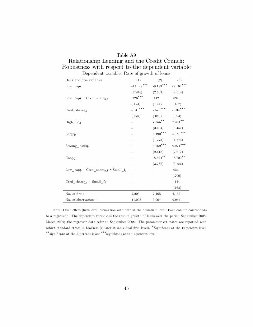
Rather than dropping large tails of the distribution of the dependentvariable in question, which in all likelihood would have resulted in the elimi-nation of observations with the most interesting information content for ourpurposes, we chose to divide the change in credit by �rm�s total assets. Thisnormalization should not alter the information content of the data, whiledelivering a variable with a much smoother distribution (see Table 1, secondrow). This is therefore the main dependent variable that we use throughoutthis paper (however, regressions with the rate of growth as the dependentvariable were also run, for the sake of robustness; see Tables A3 and A9 inAppendix II).The risk of �rms�defaulting is measured by Zscore, an indicator of the

probability of default of a given �rm, which is computed annually by theCompany Accounts Data Service (CADS) on balance sheet variables (themethodology is described by Altman, 1968, and Altman et al., 1994). It takesvalues from 1 to 9. Firms with Zscore value between 1 and 3 are considered�low risk�by CADS, those in the 4-6 range are considered �medium risk�, andthose in the 7-9 range are considered �high risk�; the latter �rms are morelikely to default within the next two years.Productivity is computed for each �rm as the log-level of (gross output)

Solow Residual, tfpi:

tfpi = ln yi � (�L � ln_li + �K � ln_ki + �M � ln_mi) , (5)

10

where ln_yi, ln_li; ln_ki and ln_mi are the logarithms of, respectively,the �rm�s gross output, hours, capital and intermediate inputs, all measuredin real terms, and the ��s are the revenue shares of each input.16 Since thelevel of productivity may vary widely across sectors, for each �rm we com-puted the di¤erence relative to the sectoral median, to allow for comparisonacross sectors.Further details on the de�nition of the variables and descriptive statistics

can be found in Appendix I.

3.2 Data sources

There are four main sources of data: those on outstanding loans come fromthe Credit Register; bank balance sheet data are drawn from the BankingSupervision Register at the Bank of Italy; data on �rms�inputs and outputs(used to measure productivity) and other �rm characteristics come from theBank of Italy annual Survey of Industrial and Service Firms and from theCompany Accounts Data Service (CADS).The Credit Register data are collected by a special unit of the Bank of

Italy (Centrale dei Rischi) and contain detailed information on virtually allindividual loans extended in Italy (see Appendix I).The Survey of Industrial and Service Firms (SISF) is carried out annually

by the Bank of Italy. The data are of very high quality, being collectedby o¢ cials of the local branches of the Bank of Italy, who often have along-standing work relationship with the �rm�s management. The CompanyAccounts Data Service (CADS - Centrale dei Bilanci) is the most importantsource of balance sheet data on Italian �rms. It covers about 30,000 �rmsand is compiled by a consortium that includes the Bank of Italy and all themajor Italian commercial banks.

16Gross-output measures of total factor productivity, whenever data are available, arepreferable to value-added measures, because of the reduced-form nature of the latter,which may induce potential model misspeci�cation and omitted variable bias when usedin regressions (see Basu and Fernald, 1997; for an analysis of these TFP measures with adataset similar to that used in this work, see Marchetti and Nucci, 2006).

11

4 Evidence for a credit crunch

4.1 The main results

The core of this paper is the investigation of loan supply e¤ects, linked tobank balance sheets, in the aftermath of Lehman�s bankruptcy, when thegrowth of credit came to a substantial halt. Within our sample, outstandingloans contracted in nominal terms by -1.1% from September 2008 to March2009. A �rst look at the data clearly suggests the importance of balancesheet factors in shaping banks�lending behavior: loans extended by banksbelonging to the lowest quartile of the capital ratio distribution decreased byroughly 20%, while credit growth for the other quartiles was positive, in the5-10% range (Table 2).

Table 2Growth of loans by bank capitalization (percent)

Variables Bank capitalization quartiles Whole

1st 2nd 3rd 4th sample

Share of total loans at Sept. 2008 32.2 30.7 10.0 27.1 100.0

Growth of loans -20.8 8.4 5.2 9.3 -1.1

The rest of this section is devoted to a more rigorous analysis of bankcapitalization e¤ects on loan supply. Consistently with the model introducedin Section 2, the basic regression for testing the credit crunch hypothesis isthe following:

�credb;i = �+ �1 � low_capb + �i + ub;i (6)

where �credb;i is the change in outstanding loans extended by bank b to�rm i between (end) September 2008 and (end) March 2009, divided bythe �rm i�s total assets in September 2008; low_capb is a dummy variablefor low-capitalized banks; �i is a �rm-speci�c �xed-e¤ect and ub;i is the re-gression residual. More precisely, low_capb is equal to 1 for banks whosetotal (risk-weighted) capital ratio is lower than 10%. The latter value is thatrecommended by the Bank of Italy, and � although the o¢ cial Basle II reg-ulatory threshold is 8% � it appears to be perceived by the market as therelevant benchmark; moreover, it roughly coincides with the 25th percentile

12

(10.5%) of the sample distribution, and is therefore also a useful referencevalue in statistical terms.17

Equation (6) includes �rm-speci�c �xed-e¤ects; this key feature allowsus to control for �rms�credit demand as well as their other characteristics.Regression results are reported in the �rst column of Table 3. The esti-mated coe¢ cient of low_capb is negative and highly signi�cant, leading to aclear rejection of the null hypothesis that a credit crunch did not occur. Wealso investigated the role of other balance sheet indicators of banks�fund-ing di¢ culties � beyond those associated with regulatory requirements �such as the liquidity ratio. We thus included the dummy variable high_liqbfor banks whose liquidity ratio (i.e., cash and securities other than shares,divided by total assets) was higher that the sample median (12.1%). Re-sults are reported in the second column of Table 3. The supply of credit bymore liquid banks is signi�cantly higher, while the estimated coe¢ cient oflow_capb remains negative and highly signi�cant.We also considered, mainly as controls, three variables related to di¤erent

aspects of banks�organization, which may have been important during thecrisis: largeb is a dummy for banks belonging to the major �ve bankinggroups (which overall extend roughly half of total loans to non-�nancial �rms,and accounted for most of the credit slowdown); scoring_bankb is a dummy,based on survey data, which is equal to 1 for banks whose use of scoringschemes in lending decisions is reported to be either �important� or �veryimportant�, and 0 for banks reporting that they make little or no use ofcredit scoring; coopb is a dummy variable for cooperative banks, which aresubject to a special regulatory regime and have been shown in the literatureto focus on relationship lending (e.g., Angelini et al., 1998).Results of the extended model are reported in the third column of Table

3. The e¤ect of bank capital and liquidity is strenghtened, despite the highsigni�cance of the estimated coe¢ cient for largeb.18 Overall, these resultsshow that the �ndings for low_capb previously reported are not due to pos-sible correlation between low bank capitalization and other banking features,such as the fact of belonging to a major banking group or the reliance on

17The use of a dummy for lowly-capitalized banks serves to capture possible non-linearities, since bank capital a¤ects credit supply only when capital constraints are bind-ing.18This �nding, as we will see, is not speci�c to the period under investigation and is

possibly related to the ongoing recomposition of market shares in the Italian credit marketfollowing the consolidation process of the sector in the �rst half of the 2000s.

13

credit scores in lending decisions.19

The contraction of loan supply by low-capitalized banks has been signi�-cant in both statistical and economic terms. The (asset-normalized) changein credit extended by low-capitalized banks is about two percentage pointslower (in annual terms) than that of other banks.20 It can be estimatedthat, on an annual basis, this corresponds to roughly 0.7% of the stock ofoutstanding loans to �rms (measured in September 2008); analogously, thee¤ect through liquidity constraints, captured by the coe¢ cient of high_liqb,corresponds to roughly 0.6% of the stock. Overall, therefore, �pure�supplye¤ects related to banks�balance sheet conditions amounted to more than1% of total credit to �rms. While this may not seem a huge impact, themacroeconomic e¤ect on output and employment may have been magni�edby the fact that many �rms, being �nancially vulnerable at the peak of therecession, were hit by the credit supply shock when the need for externalfunding was more acute and sharply rising.21

Our interpretation of the results is corroborated by looking at loan supplydevelopments in the pre-crisis period. In particular, for comparison purposes,we considered the latest September-March six-month period before the be-ginning of the turmoil (August 2007), that is September 2006-March 2007,and estimated the extended model with the corresponding data. The resultsare reported in the fourth column of Table 3: as expected, at normal timesthe supply of credit is not a¤ected by bank capitalization (or liquidity, forthat matter). Overall, the evidence reported for the pre-crisis period stronglycon�rms the interpretation of our results as evidence of a credit crunch.

19The coe¢ cient of scoring_bankb is positive and signi�cant, contrary to the commonconjecture that substantial use of credit scores would weigh negatively on lending decisionsduring a recession accompanied by a �nancial crisis. However, the procyclical implicationsof credit scoring on loan developments deserve a deeper analysis, which is beyond the scopeof this paper. Similar considerations apply to the estimate of the coe¢ cient of coopb, whichis typically interpreted as a proxy of relationship lending.20The impact on credit growth at the �rm level can be signi�cantly higher, depending

on the �rm-speci�c ratio of total assets to credit.21Counterfactual simulations with a large macroeconometric model of the Italian econ-

omy suggest that the contraction of credit supply accounted for about a quarter of the 5%decrease in Italian GDP in 2009 (see Caivano et al., 2010); credit restriction is estimatedon the basis of the spread between bank lending rates and interbank interest rates overthe 3-month horizon (Fair and Ja¤ee, 1972).

14

4.2 Robustness

The results proved extremely robust in several respects. First, they aresubstantially unchanged if the original dependent variable is replaced by therate of growth of loans (Table A3 in Appendix II). Second, the results provedrobust to the choice of the threshold value for the de�nition of low_capb(low_capb was set equal to 1 for banks whose capital ratio is lower than thesample median, i.e. 13.0; Table A4). A third set of robustness checks wasrelated to the de�nition of credit: we considered granted rather than utilizedcredit (Table A5).A further robustness exercise was related to the level at which the capital

ratio is computed (individual banks vs. group). Regulatory requirementsconcern both unconsolidated capital ratios and consolidated ones. Through-out this paper we chose to use unconsolidated ratios, in order to exploit theheterogeneity of behavior and conditions across banks belonging to the samegroup. For example, the literature on internal capital markets shows thatagency frictions among individual �rms within industrial or banking groupsgenerates relationships which tend to be similar to those observed amongindependent market participants (e.g., Shin and Stultz, 1998). Moreover,consolidated balance sheet data are not available at quarterly frequency, sothat we would have had to use capital ratios computed on either June orDecember 2008; given that capital levels were changing during the periodof interest, this could add noise to the data. At any rate, consolidated andunconsolidated capital ratios showed an extremely high level of correlation inJune 2008 (.87). A �nal advantage, on statistical grounds, is the much greatervariability and granularity of unconsolidated capital ratios.22 Nonetheless,for robustness purposes (since bank supervision activity tends to focus onconsolidated parameters), we regressed our dependent variable (computedwith consolidated loan data) on low_capb computed on the basis of con-solidated capital ratios and the corresponding distribution. The estimatedcoe¢ cient remains negative and highly signi�cant (see Table A6).A �nal robustness exercise was related to the accounting impact of secu-

ritizations on loan data. The data on outstanding loans used throughout thepaper do not include securitized loans. In principle this seems appropriatesince typically a bank, by securitizing a loan, sells the loan on the market,

22The banks of the �ve major groups (15% of our dataset) account for roughly 60% oftotal bank-�rm observations; over all those observations the �ve di¤erent values of theconsolidated capital ratio lie in a very narrow range (9.1-10.4).

15

transfering the corresponding credit risk to third parties. The loan supply ofthat bank to the given �rm decreases by the corresponding amount. However,in practice, in the period considered here most securitizations were so-calledretained-securitizations, whose only purpose was to create securities to beused as collateral in the Eurosystem�s re�nancing operations but which didnot imply any transfer of risk to third parties. In such cases the loan supplyat the bank-�rm level can be considered unchanged. We therefore adjustedloan data for the e¤ect of securitizations, by re-including loans which weresecuritized during the period of interest into the stock of outstanding bank-�rm loans at the end of March 2009.23 The results are shown in Table A7and are virtually unchanged.A full discussion of all the robustness exercises is provided in Appendix

II.

4.3 Substitution across banks

We also tried to investigate whether and to what extent borrowers wereable to compensate for the contraction of credit supplied by low-capitalizedbanks by increasing loans from other banks. In principle, in the extremecase of perfect and prompt substitution the crunch would have no e¤ects onproduction and employment, and there would merely be a recomposition ofcredit �ows within the banking sector.For each �rm in our dataset we thus computed the change of loans ex-

tended by all highly-capitalized banks (i.e., banks with a capital ratio� 10%)and regressed it on the change of loans extended by all other banks (de�nedas cred_lowcapi). If substitution were perfect and this were the only fac-tor driving the relationship being estimated, we would expect a coe¢ cientequal to -1; incomplete substitution would correspond to a coe¢ cient be-tween -1 and 0; a coe¢ cient not statistically di¤erent from 0 would imply nosubstitution, while a positive and signi�cant coe¢ cient would signal comple-mentarity between loans from the two bank categories. As it is not possibleto include �xed e¤ects, we included controls in the regression for the main�rm characteristics (i.e. risk of default, size, economic sector and region)to capture other factors which might a¤ect the relationship between the de-pendent variable and the regressor. Results (with and without controls) are

23Double-counting is not an issue since virtually all those which bought loans duringthe period examined are special purpose vehicles or other �nancial institutions which arenot included in our sample of banks.

16

reported in the �rst and second columns of Table 4. The estimated coe¢ -cient of cred_lowcapi is negative and highly signi�cant, with an absolute sizemuch lower than one, thus suggesting that some substitution did take place,but was rather limited (namely, the increase in loans from highly-capitalizedbanks appears to have compensated on average for only around 30% of thedecrease of loans from low-capitalized banks).Estimating the same regression in the pre-crisis period (September 2006-

March 2007) broadly con�rms this interpretation of the results. We expectthat at normal times, with no credit crunch, the scope for substitution wouldbe smaller, if present at all; in fact, the estimated coe¢ cient of cred_lowcapiin the comparable pre-crisis period is much smaller and its statistical signif-icance is lower (third column of Table 4).Considering again the after-Lehman period, we also found some evi-

dence that the number of lenders a¤ected borrowers� ability to substituteacross banks, as one would expect. We computed a new dummy variable,few_lendersi, for �rms that have less than 4 lenders (roughly 31% of thetotal; �rms that have at least 3 represent 22% of the total). The results arereported in the fourth column of Table 4; for the latter category of �rms, theestimated coe¢ cient of cred_lowcapi is much smaller and not statisticallysigni�cant, whereas for �rms that borrow from at least 4 lenders the estimateis highly signi�cant and very similar in size to that reported earlier.

5 Flight to quality and evergreening

5.1 Heterogeneity of credit crunch across �rms

We now turn to the investigation of a speci�c aspect of the crunch, namelythe occurrence of a �ight to quality away from risky borrowers and the het-erogeneity of this phenomenon across banks.We start by analyzing whether (and how) the impact of the crunch was

di¤erentiated across di¤erent types of �rms. We considered four main �rmcharacteristics, namely size, export propensity, risk of default and produc-tivity. The corresponding variables were interacted with low_capb, �rst oneat a time and then all together; the results are reported in Table 5. Thecontraction of loan supply from low-capitalized banks was signi�cantly morepronounced for smaller �rms (i.e., �rms with less than 50 employees, identi-�ed by the dummy small_fi). As to export propensity, there is no evidence

17

that exporting �rms (identi�ed by the dummy exporti) were hit more severelyby the crunch.24 With regard to productivity, there is no evidence that moreproductive �rms have been shielded from the crunch (tfpi is �rms�Solowresidual, sectorally de-meaned). Finally, and most interestingly for our pur-poses, there is some evidence that the contraction of credit supply has beenstronger for riskier �rms (high_riski is a dummy for �rms whose Zscore isin the 7-9 range).The evidence found for low_capb � small_fi and low_capb � high_riski

brings to mind the notion of the �ight to quality described by Bernanke et al.(1996), based on the role of agency costs. Notice however that our �ndings areslightly di¤erent, as in our analysis agency costs are captured by �rm-speci�c�xed e¤ects. The estimated coe¢ cient of low_capb � small_fi and that oflow_capb � high_riski capture an additional impact on lending to smallerand riskier �rms respectively, speci�c to poor bank capitalization, whichis not related to di¤erences in agency costs compared to other borrowers.One possible factor underlying this form of �ight to quality linked to bankcapital, as mentioned in Section 2, is the e¤ect of the higher risk-sensitivenessof Basel II capital requirements. Other potentially relevant factors includeevergreening and �patience�. The di¤erent mechanisms imply di¤erences inlending patterns across banks, according to size and organization.

5.2 Flight to quality: Heterogeneity across banks

A �rst dimension to be investigated is bank size. In the Italian bankingsector � as in most developed banking sectors worldwide � small, localbanks coexist with large, multi-national banking groups. The divergencesin bank�s organization and decision-making are likely to a¤ect the attitudetowards borrower risk. For example, with regard to evergreening, providing�cheap�credit to a borrower with a high risk of default, in order to postponecredit losses, is presumably easier for a smaller bank where discretion inlending decisions is higher and the weight of credit scoring is lower than for alarger bank, where lending decisions are based on more automatic procedures.Indeed, by introducing bank size into our analysis of lending patterns to riskyborrowers, a clear di¤erence emerges. Consider the following regression:

24Given that these �rms have been hit hard by the collapse of world demand, this is aninteresting �nding since it appears to contradict concerns that �short-termist�banks mightpossibly reduce credit to these �rms, which represent the dynamic and healthy core of theItalian productive system.

18

�credb;i = �+ �1 � low_capb + �2 � (low_capb � high_riski) (7)

+�3 � [low_capb � high_riski � (1� largeb)] + �4 � largeb+�i + "b;i .

The results are reported in the second column of Table 6. Given the spec-i�cation of this model � namely the presence of the triple interaction termlow_capb �high_riski �(1� largeb) � the coe¢ cient of low_capb �high_riskicaptures the �ight to quality e¤ect (i.e. the reallocation of credit awayfrom riskier borrowers) for larger banks alone. Its coe¢ cient is negativeand highly signi�cant; interestingly, this means that the evidence of a re-allocation away from riskier borrowers is much stronger for larger banks(both in size and statistical signi�cance) than for the average low-capitalizedbank (�rst column of Table 6).25 On the other hand, the coe¢ cient oflow_capb � high_riski � (1� largeb) is positive and highly signi�cant, show-ing that the lending pattern to riskier borrowers by smaller low-capitalizedbanks is signi�cantly di¤erent from that of larger banks � namely, the �ightto quality of smaller banks is less pronounced than that of larger banks.Moreover, for such smaller (low-capitalized) banks there is no evidence atall of a �ight to quality, since the total reallocation e¤ect towards riskierborrowers by such banks is given byc�2+c�3, which is non-negative.26 Impor-tantly, all the results are robust to the inclusion in the regression of all doubleinteractions among the variables in the equation (third column of Table 6).27

As anticipated throughout the paper, there are at least three possible ex-planations for the �nding that, in striking contrast with larger low-capitalizedbanks, smaller ones have not reallocated their credit away from riskier bor-rowers after Lehman.25The �rst column of Table 5 reports again, for comparison purposes, the regression

presented in the fourth column of Table 4.26In mathematical terms, it can readily be seen that, for smaller banks (i.e. those for

which largeb=0), @@ ch a n g e o f lo a n s

@ l ow _ c a p

@ high_risk = c�2+ c�3. Indeed, based on this regression there isevidence of a �ight to risk for smaller banks, since c�2+ c�3=0.504, with the hypothesisof c�2+ c�3 = 0 being rejected at the 1% statistical level (F-statistic=13.38, with p-value.000).27The positive coe¢ cient for low_capb � (1� largeb) signals that the e¤ect of capital on

lending is more important for larger banks. This may re�ect di¤erent ownership patterns(which may interfere with banks�ability to adjust their capital promptly) or more carefulmonitoring by market participants of larger and listed banks.

19

One explanation is that, compared to larger banks, smaller ones are lessa¤ected by the new Basle II risk-sensitive capital requirements and did notreallocate their loan portfolio at all to save on scarce capital. Another poten-tial explanation is evergreening, on the ground that, as already mentioned,reallocation of credit in favor of borrowers with a bad credit score � �nal-ized to avoid or postpone the realization of losses � is presumably easierfor smaller banks. A third possible explanation is that smaller banks havebetter (soft) information on riskier borrowers, compared to larger banks; thiswould allow smaller banks to keep funding borrowers with bad credit scoresthat have good economic fundamentals and are just undergoing temporary�nancial di¢ culties. If this is so, the lack of ��ight from risk�by smallerbanks would be evidence of virtuous �patience�, as opposed to suboptimalmyopia (short-termism) on the part of larger banks.28

As to the �rst explanation, when the adoption of Basle II is completed,some technical aspects of the new capital requirements will almost certainlydeliver a higher risk-sensitiveness by larger banks (which are more likely toadopt the �internal rating system�). However, the implementation has beengradual and, in the period under consideration, was still partial.29 It there-fore appears unlikely that the divergences documented above are entirelyjusti�ed by the e¤ect of Basle II regulation. While the latter e¤ect may bean interesting issue for future research, in the rest of this section we conductother exercises aimed at disentangling the �evergreening�explanation fromthat based on �patience�.

5.3 Corroborating the �evergreening�explanation

As just argued, the �ndings of the second and third columns of Table 6 mightre�ect �patience�by smaller low-capitalized banks � as opposed to myopiaon the part of larger banks � instead of evergreening. Indeed, this is a

28This interpretation, however, seems inconsistent with the negative and signi�cantcoe¢ cient for (1� largeb) �high_riski, which suggests that the lenience of smaller lenderstowards risky borrowers is speci�c to the lowly capitalized smaller intermediaries.29The sensitivity of new capital requirements to the risk of individual borrowers is

maximized under the �internal ratings-based�(IRB) approach, which is typically chosenby larger banks. Under the alternative system (�standardized�approach), all borrowersthat are not rated by the rating agencies are given the same weight in the computationof capital requirements, regardless of the actual individual risk pro�le. The share of loanscovered by the IRB system in the period September 2008-March 2009 for the few (largeand small) banks which adopted it varied between roughly 40 and 70%.

20

general limitation of all balance sheet indicators of borrowers�quality thatare used in the evergreening literature, arising from the fact that they donot take into any account �rms� future prospects.30 Thus, by using thesemeasures, it is not possible to distinguish true forbearance lending from e¢ -cient debt restructuring, whereby a non myopic lender helps a borrower, whois currently distressed but whose expected pro�tability is potentially high,overcome temporary di¢ culties. The latter would typically be the case of a�rm which got involved in substantial restructuring, funded by debt, thanksto which it recovers its competitiveness.31

A simple but quite powerful method for discriminating between the twoalternative explanations is to supplement the information of (�nancially-focused) balance sheet indicators with that of indicators which are, arguably,better proxies of the �rm�s economic fundamentals and competitiveness, andtherefore more forward-looking measures of its economic prospects, such asproductivity.We therefore replicated the regressions reported in Table 6 by replacing

high_riski with a proxy for bad (impaired) borrowers, imp_bori, which isequal to 1 if high_riski=1 and, at the same time, the �rm�s Solow residual,sectorally de-meaned, is lower than the sample median. Having identi�edbad borrowers in this way, any evidence of reallocation of credit towardsthem (or weaker reallocation away from them) can hardly be interpretedas evidence of �patience�. The results with imp_bori are reported in Table7 (whose structure replicates that of Table 6; they strongly con�rm, andpossibly strengthen, previous evidence. The ��ight from bad borrowers�by

30An alternative approach to the identi�cation of impaired borrowers has been adoptedby Caballero et al. (2008). In that paper, bad borrowers are identi�ed as those receivingan interest rate subsidy, which in turn is identi�ed by comparing, for any �rm and yearin the sample, total interest expenses with an estimated lower bound. As it is not basedon indicators of current performances, this approach o¤ers the main advantage of beinginherently more forward-looking. Another more forward-looking measure adopted is stockreturns, as in Peek and Rosengren (2005). The main limitation in this case is that suchinformation can be obtained only for listed �rms, which tend to be only large �rms. Also,one could argue that during crises stock prices are not as e¢ ciently determined as innormal times.31There is speci�c evidence that this factor may have been relevant in our context.

Bugamelli et al. (2008) document, by analyzing a dataset including our sample of �rms,that substantive �rms�restructuring occurred in the Italian manufacturing and servicessectors in the last decade, as a response to the introduction of the euro and the need toface global competition.

21

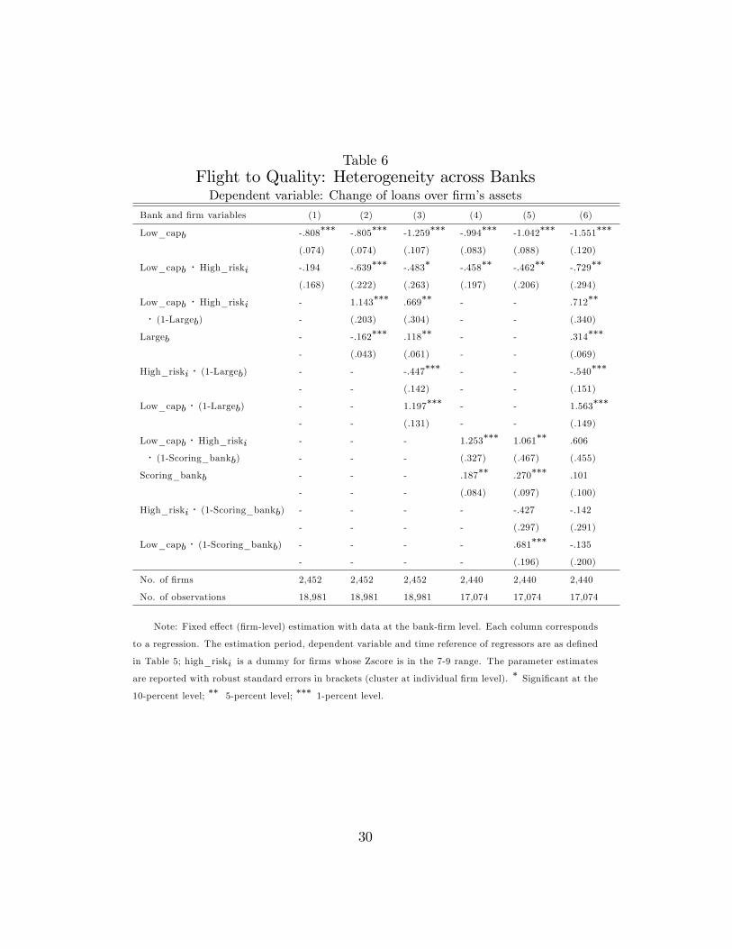
larger banks, captured by the estimated coe¢ cient of low_capb � imp_boriin columns 2-3, has intensi�ed (the size of the coe¢ cient is roughly doublethat of Table 6). The coe¢ cient of low_capb � imp_bori � (1� largeb), whichcaptures the di¤erence between the behavior of smaller and larger banks, hasremained positive and highly signi�cant; if anything, its size appears to haveincreased sharply as well. Overall, again, there is no evidence of a ��ight frombad borrowers�by smaller banks (i.e. the hypothesis ofc�2+ c�3=0 cannot berejected).32

Notice that the �ndings documented in the second and third columns ofTable 7 also lend support to the explanation based on evergreening as againstthat based on Basle II regulations. In fact, if the lack of a �ight to quality forsmaller banks (documented in Table 6) were justi�ed only by the di¤erentialimpact of new capital requirements, including borrowers�productivity in theanalysis should leave the results broadly unchanged, since the rating methodsused under the IRB approach typically focus on balance sheet variables (suchas those summarized in Zscore), and do not take into account measures of�rms�productivity and competitiveness. If anything, the use of imp_boriinstead of high_riski should attenuate the observed di¤erence between largeand small banks, since, in the absence of evergreening, small banks shouldreallocate their credit away from the �bad borrowers�identi�ed by imp_borieven if that does not give them the full advantages, in terms of lower risk-weighted capital ratios, brought by Basle II and enjoyed by larger banks. Aswe saw, on the contrary, the observed di¤erence between larger and smallerbanks widened.Going back to the comparison between the �evergreening�and the �pa-

tience� explanations, another way of testing the hypothesis that loans toriskier borrowers might actually represent good pro�t opportunities � withsmaller low-capitalized banks being in a better position to detect them �is by looking at interest rate developments at the bank-�rm level. This is

32A further robustness exercise is the following. Since the aim is to investigate theextension of credit to risky borrowers for the purpose of avoiding losses on pre-existingloans, it is appropriate to include, among the borrowers which may potentially bene�t fromevergreening, only �rms which, at the beginning of the period considered (i.e., September2008), were actively borrowing from a given bank. To this end, we estimated the regressionsreported in Table 6 after dropping the bank/�rm observations associated with �rms withimp_bori =1 and no outstanding loans from a given bank. After doing this, the dummyimp_bori identi�es (only and all) the potential recipients of �evergreening� loans. Theresults are substantially unchanged and are reported in Table A7 in Appendix II.

22

feasible since we have information on average nominal interest rates for eachbank-�rm relationship over the same period. The rationale for looking atinterest rates is that �genuine�loans (i.e. not associated with evergreening)to riskier but pro�table borrowers should be associated with higher inter-est rates. On the contrary, interest rates on the loans extended by smallerlow-capitalized banks to riskier borrowers turned out not to be statisticallydi¤erent from those on other loans. See Table 8, which for the sake of sim-plicity replicates the structure of Tables 5, with the dependent variable beingreplaced by interest rates at the bank-�rm level (average over the period inquestion). For our purposes, we do not need to provide a structural inter-pretation of all the parameters in the regression; we simply notice that theestimated coe¢ cient of low_capb � high_riski � (1 � largeb) is clearly notstatistically di¤erent from zero (second and third columns of Table 8).

5.4 The role of credit scoring

We have provided evidence corroborating the interpretation of our �ndingsbased on forbearance lending. When initially putting forward this hypothesis,we mentioned that one reason why evergreening might be easier for smallerbanks is the lower weight assigned to credit scoring techniques. It seems nat-ural, therefore, to re-estimate previous regressions after replacing (1�largeb)with (1�scoring_bank). The results are documented in the fourth and �fthcolumns of Tables 5, 6 and 7 (which replicate the second and third columnsof the corresponding tables). The �ndings clearly con�rm those obtainedwith (1 � largeb). Namely, banks which rely extensively on credit scoringdid reallocate credit away from risky (bad) borrowers, while the others didnot (Tables 5 and 6). For the sake of comparing the explanatory power of(1� largeb) with that of (1�scoring_bank) in capturing the allegedly �ever-greening�e¤ect, we also included all regressors in the same equation. The re-sults, reported in the sixth column of Tables 5 and 6, show that the estimatedcoe¢ cient of [low_capb �high_riski �(1�largeb)]maintains its high statisticalsigni�cance, unlike that of [low_capb �high_riski �(1�scoring_bank)]. Thissuggests that the weight of credit scoring was only one of the factors under-lying our �ndings; additional factors associated with bank size played a role,presumably related to organizational aspects. For example, the importanceof agency costs in major groups, documented in the literature (e.g., Stein,2002), might induce a tendency to centralize decision processes and perma-nently limit the autonomy of local loan o¢ cers, possibly making evergreening

23

more di¢ cult.33

6 Capital crunch and relationship lending

Finally, we investigated whether and how the capital crunch documented inSection 4 is a¤ected by the intensity of bank-�rm relationships. We did soby supplementing the main regressions with the share of credit that a given�rm receives from a given bank, cred_shareb;i, alone and interacted withlow_capb. The results for the model without and with controls are reported,respectively, in the �rst and second columns of Table 9. The estimated coef-�cients of low_capb � cred_shareb;i and cred_shareb;i are both negative andstatistically signi�cant.34 Overall, therefore, we �nd no evidence that thecrunch has been attenuated by intense bank-�rm relationships, or, more ingeneral, that credit supply during the turmoil has been positively a¤ectedby relationship lending.35 This is consistent with the �nding by Peek andRosengreen (2005) that main banks were less likely to increase lending com-pared to other banks during the �lost decade�in Japan. At least partially,this pattern may re�ect, an attempt by such banks to diversify credit risk inthe context of a severe �nancial crisis.Notice, however, that our analytical framework is not well suited for an

analysis of relationship lending, which is not the aim of this paper. First,the non-negligible category of �rms borrowing from a single lender � forwhich relationship lending is most valuable � is excluded by our analysis,based on the use of �rm-level �xed e¤ects which requires multiple lenders.Moreover, for the �rms included in our analysis some of the e¤ects of lendingrelationships might be captured by the �xed e¤ects. For example, the pres-ence of a main bank may provide some kind of �certi�cation�allowing otherintermediaries to lend to the same �rm, at lower interest rates, while savingon monitoring costs.36

33As to Table 7, the estimated coe¢ cient of low_capb �high_riski �(1�scoring_bankb)is negative but mostly not statistically signi�cant, showing that interest rates on the riskierloans extended by low-capitalized banks which make little use of scoring techniques arenot higher than those on other loans.34Similar evidence has been obtained by analyzing credit �ows to smaller �rms, which

typically bene�t more from relationship lending (third column of Table 8).35Substantially similar results have been obtained by using the rate of growth of loans

as the dependant variable (see Table A8).36See Casolaro and Mistrulli (2008). In general, an analysis of the role of relationship

24

We also investigated the link between the intensity of bank-�rm rela-tionships and the patterns of lending to risky borrowers. We run the mainregressions reported in Table 7 after including cred_shareb;i, respectivelyalone and interacted with [low_capb � imp_bori � (1� largeb)] and [low_capb �imp_bori �(1�scoring_bankb)]. The results are reported in Table 10; there isno evidence that the (supposedly) �evergreening�e¤ect is either strengthenedor weakened by relationship lending.

7 Conclusions

In this paper we have presented evidence of a credit crunch, associated withlow bank capitalization and scarce liquidity, over the 6-month period follow-ing Lehman�s bankruptcy.We have shown that the dampening e¤ect on credit supply of low-capitalized

banks was quite sizeable; moreover, we o¤er some evidence to the e¤ect thatthe ability of borrowers to substitute loans from low-capitalized banks withloans from the other banks has been limited, and almost nil in the case of�rms that borrow from only a few lenders.By analyzing the impact of the crunch across di¤erent types of �rms,

we also found that larger low-capitalized banks reallocated their credit awayfrom riskier �rms. Quite strikingly, this ��ight to quality�was not observedfor smaller low-capitalized banks.A �rst explanation for this dichotomy hinges on the potentially di¤erent

impact of Basle II capital regulations on larger vs. smaller banks; however,the implementation of the new, more risk-sensitive capital requirements wasstill partial during the period of interest, and appears unlikely to justify allthe di¤erence in the observed ��ight to quality�. Another potential explana-tion hinges on evergreening. The rationale is that evergreening is arguablyeasier for smaller banks, whose lending decision processes are more �exibleand less constrained by credit scores, than for larger banks. A third poten-tial explanation is �patience�by smaller banks, in the sense described in thispaper. In order to disentangle between the two last explanations we useddata on borrowers�productivity and interest rates at bank-�rm level. The

lending cannot neglect �rms�bank-invariant characteristics. De Mitri et al. (2009) conductan analysis along these lines based on Italian �rm-level data (that include our sample);they �nd a positive link between several measures of relationship lending and �rms�creditavailability after Lehman.

25

evidence suggests that evergreening by smaller lenders did take place, point-ing to a trade-o¤ vis-à-vis an excessively procyclical lending supply by largerbanks.Overall, this paper innovates by combining two separate strands of the

literature on bank capital and lending supply, namely those on the capitalcrunch and evergreening. Our results indicate that pressure on bank capi-tal may simultaneously produce two opposite lending biases. A generalizedexcessive tightening (crunch) and some excessive loosening of credit policiestowards risky borrowers (evergreening) may well coexist, representing twodi¤erent facets of banks�response to capital contraints.

26

Table 3Testing for a Credit Crunch

Dependent variable: Change of loans over �rm�s assets

Bank (1) (2) (3) (4)

variables Pre-crisis

Low_capb -.835�� -.867�� -1.086�� .036

(.066) (.067) (.076) (.047)

High_liqb - .447�� .560�� -.078

- (.084) (.144) (.096)

Largeb - - -.142�� -.090�

- - (.045) (.049)

Scoring_bankb - - .219�� .105

- - (.088) (.072)

Coopb - - -.439�� -.003

- - (.137) (.130)

No. of �rms 2,558 2,558 2,546 2,358

No. of observations 19,576 19,576 17,596 16,602

Note: Fixed e¤ect (�rm-level) estimation with data at the bank-�rm level. Each column corresponds

to a regression. The dependent variable is the change of loans from individual banks over the period

September 2008-March 2009, normalized to �rm�s assets; the regressor data refer to September 2008.

In column 4, the dependent variable is de�ned over the period September 2006-March 2007, and the

regressor data refer to September 2006. The parameter estimates are reported with robust standard

errors in brackets (cluster at individual �rm level).�Signi�cant at the 10-percent level; ��signi�cant at the 5-percent level; ��signi�cant at the 1-percent

level.

27

Table 4Substitution across Banks

Dependent variable:Change of loans from highly-capitalized banks over �rm�s assets

Firm variables (1) (2) (3) (4)

Pre-crisis

Cred_lowcapi -.306�� -.297�� -.096� -

(.067) (.070) (.051) -

Cred_lowcapi � (1-Few_lendersi) - - - -.316��

- - - (.083)

Cred_lowcapi � Few_lendersi - - - -.166

- - - (.107)

Few_lendersi - - - -.753��

- - - (.360)

Credit risk dummies No Yes Yes Yes

Size dummies No Yes Yes Yes

Sectoral dummies No Yes Yes Yes

Regional dummies No Yes Yes Yes

No. of �rms/observations 2,558 2,452 2,371 2,452

Note: OLS estimation with �rm-level data. Each column corresponds to a regression. In columns 1,

2 and 4 the dependent variable is the change of loans from highly-capitalized banks, normalized to �rm�s

assets, de�ned over the period September 2008-March 2009, and the regressor data refer to September

2008; in column 3 the dependent variable is de�ned over the period September 2006-March 2007 and the

regressor data refer to September 2006. The parameter estimates are reported with robust standard errors

in brackets (cluster at individual �rm level). The credit risk dummies identify �rms whose Zscore value

is between, respectively, 1 and 3 (�low risk�), 4 and 6 (�medium risk�) and 7 and 9 (�high risk�) . The

size dummies identify four categories of �rms: 20-50 employees, 51-200 employees, 201-1000 employees,

over 1000 employees. The sector dummies refer to 2-digit sectors. The regional dummies refer to four

macro-regions: North-West, North-East, Center and South.�Signi�cant at the 10-percent level; ��signi�cant at the 5-percent level; ��signi�cant at the 1-percent

level.

28

Table 5Heterogeneity of the Crunch across FirmsDependent variable: Change of loans over �rm�s assets

Bank and �rm variables (1) (2) (3) (4) (5)

Low_capb -.744�� -.799�� -.964�� -.808�� -1.032��

(.069) (.143) (.116) (.074) (.201)

Low_capb � Small_fi -.384�� - - - -.460��

(.180) - - - (.211)

Low_capb � Exporti - -.050 - - .011

- (.161) - - (.186)

Low_capb � Tfpi - - .227 - .191

- - (.138) - (.157)

Low_capb � High_riski - - - -.194 -.367�

- - - (.168) (.190)

High_liqb - - - - .583��

- - - - (.145)

Largeb - - - - -.145��

- - - - (.045)

Scoring_bankb - - - - .195��

- - - - (.089)

Coopb - - - - -.441��

- - - - (.138)

No. of �rms 2,558 2,558 2,558 2,452 2,440

No. of observations 19,576 19,576 19,576 18,981 17,074


to a regression. The dependent variable is the change of loans from individual banks, normalized to �rm�s

assets, de�ned over the period September 2008-March 2009. The regressor data refer to, respectively,

September 2008 for bank variables and 2007 averages for �rm variables. The parameter estimates are

reported with robust standard errors in brackets (cluster at individual �rm level). Small_fi is a dummy

for �rms with less than 50 employees; exporti is a dummy for exporting �rms (roughly 70% of the total);

high_riski is a dummy for �rms with a high risk of default (as signalled by a Zscore value between 7 and

9), and tfpi is a dummy for �rms whose total factor productivity (de-meaned at sectoral level) is higher

than the median.�Signi�cant at the 10-percent level; ��signi�cant at the 5-percent level; ��signi�cant at the 1-percent

level.

29

Table 6Flight to Quality: Heterogeneity across BanksDependent variable: Change of loans over �rm�s assets

Bank and �rm variables (1) (2) (3) (4) (5) (6)

Low_capb -.808�� -.805�� -1.259�� -.994�� -1.042�� -1.551��

(.074) (.074) (.107) (.083) (.088) (.120)

Low_capb � High_riski -.194 -.639�� -.483� -.458�� -.462�� -.729��

(.168) (.222) (.263) (.197) (.206) (.294)

Low_capb � High_riski - 1.143�� .669�� - - .712��

� (1-Largeb) - (.203) (.304) - - (.340)

Largeb - -.162�� .118�� - - .314��

- (.043) (.061) - - (.069)

High_riski � (1-Largeb) - - -.447�� - - -.540��

- - (.142) - - (.151)

Low_capb � (1-Largeb) - - 1.197�� - - 1.563��

- - (.131) - - (.149)

Low_capb � High_riski - - - 1.253�� 1.061�� .606

� (1-Scoring_bankb) - - - (.327) (.467) (.455)

Scoring_bankb - - - .187�� .270�� .101

- - - (.084) (.097) (.100)

High_riski � (1-Scoring_bankb) - - - - -.427 -.142

- - - - (.297) (.291)

Low_capb � (1-Scoring_bankb) - - - - .681�� -.135

- - - - (.196) (.200)

No. of �rms 2,452 2,452 2,452 2,440 2,440 2,440

No. of observations 18,981 18,981 18,981 17,074 17,074 17,074


to a regression. The estimation period, dependent variable and time reference of regressors are as de�ned

in Table 5; high_riski is a dummy for �rms whose Zscore is in the 7-9 range. The parameter estimates

are reported with robust standard errors in brackets (cluster at individual �rm level). � Signi�cant at the

10-percent level; �� 5-percent level; �� 1-percent level.

30

Table 7Corroborating the �Evergreening�ExplanationDependent variable: Change of loans over �rm�s assets


Low_capb -.792�� -.789�� -1.256�� -.995�� -1.057�� -1.574��

(.068) (.068) (.100) (.077) (.082) (.112)

Low_capb � Imp_bori -.671�� -1.266�� -1.158�� -.992�� -.947�� -1.423��

(.277) (.360) (.413) (.330) (.342) (.462)

Low_capb � Imp_bori - 1.676�� 1.402�� - - 1.657��

� (1-Largeb) - (.346) (.486) - - (.569)

Largeb - -.197�� .158�� - - .360��

- (.040) (.057) - - (.064)

Imp_bori � (1-Largeb) - - -.589�� - - -.710��

- - (.213) - - (.233)

Low_capb � (1-Largeb) - - 1.212�� - - 1.564��

- - (.121) - - (.137)

Low_capb � Imp_bori - - - 1.292�� .645 -.350

� (1-Scoring_bankb) - - - (.380) (.564) (.563)

Scoring_bankb - - - .145� .346�� .154

- - - (.083) (.099) (.100)

Imp_bori � (1-Scoring_bankb) - - - - .003 .446

- - - - (.338) (.321)

Low_capb � (1-Scoring_bankb) - - - - .836�� .009

- - - - (.189) (.190)

No. of �rms 2,452 2,452 2,452 2,440 2,440 2,440




in Table 5; imp_bori is a dummy for �rms whose Zscore is in the 7-9 range and whose productivity

(sectorally de-meaned) is lower than the sample median. The parameter estimates are reported with

robust standard errors in brackets (cluster at individual �rm level). � Signi�cant at the 10-percent level;�� 5-percent level; �� 1-percent level.

31

Table 8Evergreening: Robustness on Interest RatesDependent variable: Interest rates at the bank-�rm level


Low_capb .031 .028 .041 .039 .019 .063

(.030) (.030) (.038) (.031) (.032) (.039)

Low_capb � High_riski -.032 -.001 -.034 .003 .003 .014

(.067) (.074) (.084) (.069) (.071) (.089)

Low_capb � High_riski - -.064 .019 - - -.169

� (1-Largeb) - (.093) (.129) - - (.135)

Largeb - -.035 -.054 - - -.068�

- (.028) (.038) - - (.040)

High_riski � (1-Largeb) - - -.070 - - -.010

- - (.083) - - (.085)

Low_capb � (1-Largeb) - - -.032 - - -.124�

- - (.060) - - (.064)

Low_capb � High_riski - - - -.325�� -.310 -.303�

� (1-Scoring_bankb) - - - (.151) (.210) (.213)

Scoring_bankb - - - -.027 -.003 .037

- - - (.049) (.060) (.062)

High_riski � (1-Scoring_bankb) - - - - -.231� -.222�

- - - - (.123) (.126)

Low_capb � (1-Scoring_bankb) - - - - .227� .291��

- - - - (.118) (.122)

No. of �rms 2,294 2,294 2,294 2,279 2,279 2,279




in Table 5; high_riski is a dummy for �rms whose Zscore is in the 7-9 range. The parameter estimates

are reported with robust standard errors in brackets (cluster at individual �rm level). � Signi�cant at the

10-percent level; �� 5-percent level; �� 1-percent level.

32

Table 9The Capital Crunch and Relationship LendingDependent variable: Change of loans over �rm�s assets

Bank and �rm variables (1) (2) (3)

Low_capb -.656�� -.785�� -.799��

(.073) (.083) (.083)

Low_capb � Cred_shareb;i -.019�� -.030�� -.026��

(.008) (.008) (.010)

Cred_shareb;i -.031�� -.028�� -.025��

(.004) (.004) (.005)

High_liqb - .434�� .431��

- (.127) (.128)

Largeb - -.227�� -.228��

- (.049) (.049)

Scoring_bankb - .113 .112

- (.088) (.088)

Coopb - -.451� -.447��

- (.140) (.140)

Low_capb � Cred_shareb;i � Small_fi - - -.020�

- - (.012)

Cred_shareb;i � Small_fi - - -.012

- - (.010)

No. of �rms 2,552 2,536 2,536

No. of observations 18,378 16,501 16,501



in Table 5. The parameter estimates are reported with robust standard errors in brackets (cluster at indi-

vidual �rm level). �Signi�cant at the 10-percent level; ��signi�cant at the 5-percent level; ��signi�cant

at the 1-percent level.

33

Table 10Evergreening and Relationship Lending



Low_capb -1.307�� (.091) -1.117�� (.076) -1.645�� (.103)

Low_capb � Imp_bori -1.042�� (.400) -.875�� (.331) -1.298�� (.445)

Low_capb � Imp_bori � (1-Largeb) .961� (.524) - 1.526�� (.650)

Low_capb � Imp_bori .025 (.023) - -.008 (.031)

� (1-Largeb)� Cred_shareb;iLargeb .094 (.058) - .296�� (.065)

Cred_shareb;i -.038�� (.004) -.039�� (.004) -.039�� (.004)

Imp_bori � (1-Largeb) -.358 (.230) - -.506 (.264)

Low_capb � (1-Largeb) 1.233�� (.115) - 1.583�� (.133)

Low_capb � Imp_bori � (1-Scoring_bankb) - .142 (.700) -1.072 (.830)

Low_capb � Imp_bori - .031 (.020) .050 (.038)

� (1-Scoring_bankb)� Cred_shareb;iScoring_bankb - .296�� (.099) .150 (.100)

Imp_bori � (1-Scoring_bankb) - .218 (.352) .540 (.345)

Low_capb � (1-Scoring_bankb) - 1.053� (.194) 1.053� (.194)

No. of �rms 2,444 2,426 2,426




in Table 5. The parameter estimates are reported with robust standard errors in brackets (cluster at

individual �rm level). � Signi�cant at the 10-percent level; �� 5-percent level; �� 1-percent level.

34

A Appendix I: Data sources, de�nition of vari-ables and some descriptive statistics

Bank and credit variables. The data on outstanding loans come from theItalian National Credit Register, maintained at the Bank of Italy. For eachborrower, banks have to report to the Register, on a monthly basis, theamount of each loan, respectively granted and utilized, for all loans exceedinga given threshold.37 The sample of banks is given by the set of intermediariesreporting a positive amount of credit utilized or extended to at least one �rmin the sample of �rms on either end-September 2008 or end-March 2009 orat both dates. Data on banks�balance sheets refer to the end of September2008. Summary statistics on the variables are reported in Table A1. Totalassets are expressed in millions of euros. The capital ratio is computed as theratio of total capital to risk-weighted assets and is expressed in percentagepoints. The numerator of the liquidity ratio is the sum of the amount ofcash and securities other than shares, the denominator is total assets. Netinterbank liabilities are expressed as a ratio of total assets. The �gures forthe �ve major banking groups refer to the set of banks belonging to the �velargest bank holding companies. The data for cooperative �rms refer to smalllocal cooperative banks subject to a speci�c regulatory regime.

Firm variables. The data on employment and hours, labor compensation,investment and capital stock are drawn from the Survey of Industrial andService Firms (SISF), carried out annually by the Bank of Italy. The dataon gross production, purchases of intermediate goods and inventories of �n-ished goods are drawn from the Company Accounts Data Service (CADS -Centrale dei Bilanci). Total factor productivity (on a gross-output basis) iscomputed as follows. Gross output is measured as the value of �rm-level pro-duction (source: CADS) de�ated by the sectoral output de�ator computed byIstat (the National Statistical Institute). Employment is the �rm-level aver-age number of employees over the year (source: SISF); �rm-level man-hoursinclude overtime hours (source: SISF). Intermediate inputs are measuredas �rm-level net purchases of intermediate goods of energy, materials andbusiness services (source: CADS), de�ated by the corresponding industryde�ator computed by Istat. Investment is �rm-level total �xed investment

37The threshold was equal to euro 75,000 until December 2008 and was then reduced toeuro 30,000.

35

in buildings, machinery and equipment and vehicles, plus investment in soft-ware and patents, (source: SISF), de�ated by the industry�s Istat investmentde�ator. Capital is the beginning-of-period stock of capital equipment andnon-residential buildings at 1997 prices. To compute it, we applied the per-petual inventory method backwards by using �rm-level investment data fromSISF and industry depreciation rates from Istat. The benchmark informa-tion is that on the capital stock in 1997 (valued at replacement cost), whichwas collected by a special section of the SISF Survey conducted for thatyear. The capital de�ator is the industry capital de�ator computed by Istat.Descriptive statistics on selected �rm variables are reported in the Table A2.

Table A1Summary statistics of bank variables(percent, unless otherwise indicated)

Five largest banking groups (62 banks) 25th pctile median 75th pctile mean

Total assets (milions of euro) 2436 10553 24716 30427

Capital ratio 8.9 10.2 12.6 12.1

Liquidity ratio 4.9 6.5 8.3 7.3

All banks (488 banks)

Total assets (milions of euro) 288 716 2384 6073

Capital ratio 10.5 13.0 16.8 15.0

Liquidity ratio 6.5 11.2 17.1 12.3

Source: Banking Supervision Register; the data refer to September 2008.

Table A2Summary statistics of �rm variables(percent, unless otherwise indicated)

Variable 25th pctile median 75th pctile mean

Number of employees (units) 45 93 233 357

Real gross output growth -3.8 3.1 10.9 4.2

TFP growth -1.6 .6 3.0 .7

TFP level (log-di¤erence from sectoral median) -12.7 5.1 18.8 .4

Labor revenue-share 9.6 15.5 22.9 18.4

Capital revenue-share 4.7 8.1 12.8 10.0

Materials revenue-share 64.0 74.8 83.1 71.6

Source: SISF and CADS; the data refer to 2007.

36

A Appendix II: Robustness

This section brie�y documents a number of robustness exercises conductedon the results presented in Sections 4 and 5, all of which have been referredto in the main text.A �rst set of exercises investigated the robustness, along four di¤erent di-

mensions, of the evidence of a credit crunch reported in Table 3. We replacedthe original dependent variable with the rate of growth of loans; the resultsare reported in Table A3 (extreme values of the dependent variable wereeliminated by dropping the top and bottom 5% of the distribution).38 Wecomputed low_capb based on the median capital ratio (13.0) as the thresh-old, instead of the 25th percentile; see Table A4 (the size of the coe¢ cientis lower, as expected, since the number of banks involved in the estimationof the e¤ect has doubled, and includes banks with relatively high capitalratios). We changed the de�nition of credit, by replacing outstanding loans,in the original dependent variable, with total credit lines (utilized and non-utilized); see Table A5 (it may be argued that this is a preferable indicator ofcredit supply, since their level is chosen mainly by banks, whereas short-termdevelopments of outstanding loans may also re�ect the choice of �rms, whichcan increase or decrease the degree of utilization of existing credit lines). Werun the baseline regression with consolidated data (both the dependent vari-able and the regressor low_capb); see Table A6. We also adjusted loan datafor the accounting e¤ect of securitizations, by re-including loans securitizedfrom October 2008 to March 2009 into the stock of outstanding bank-�rmloans at March 2009 (see Section 4.2 for a discussion of the rationale); seeTable A7.A second set of exercises investigated the robustness (with respect to the

38This robustness check is important since our choice of the dependent variable mightpotentially a¤ect the identi�cation of �rm-speci�c e¤ects within our model. Consider, forexample, what would happen if �weak�(undercapitalized) banks were specialized, beforethe crisis, in �weak��rms (hit hardest by the crisis). Given the de�nition of our benchmarkdependent variable (i.e., absolute changes in credit), the values of such variable might beof a di¤erent order of magnitude across banks exposed to a di¤erent degree towards agiven �rm or category of �rms, and in principle our �rm-speci�c �xed-e¤ects might fallshort of fully capturing demand e¤ects. In such case, the observations related to the banksmost exposed with �weak��rms (associated with the largest absolute changes in credit)might possibly drive the estimate of the coe¢ cient of low_capb. The results with the rateof growth of loans as the dependent variable rule out this potential explanation of ourresults.

37

dataset) of the evidence on evergreening reported in Table 7. We included,among the borrowers that potentially bene�t from evergreening, only �rmswhich, at the beginning of the period considered, were actively borrowingfrom a given bank. To this purpose, we estimated the regressions reportedin Table 7 after dropping the (few) observations associated with �rms withimp_bori =1 and no outstanding loans from a given bank at September 2008.By doing so, the dummy imp_bori identi�es (only and all) the potentialrecipients of �evergreening�loans. See Table A8.Finally, we checked the robustness of the evidence on relationship lending

with respect to the de�nition of the dependent variable; namely, we repli-cated the evidence reported in Table 9 after replacing the original dependentvariable with the rate of growth of loans. See Table A9.

38

Table A3The Credit Crunch:

Robustness with respect to the dependent variableDependent variable: Rate of growth of loans

Bank (1) (2) (3) (4)


Low_capb -9.123�� -9.025�� -7.572�� -2.406

(1.552) (1.606) (1.754) (1.550)

High_liqb - -.856 7.786�� -2.273

- (2.396) (3.473) (3.872)

Largeb - - 4.302�� -2.753�

- - (1.766) (1.631)

Scoring_bankb - - 9.091�� 4.285��

- - (2.612) (2.898)

Coopb - - -8.498�� 8.189

- - (3.811) (6.426)

No. of �rms 2,205 2,205 2,165 2,028



to a regression. The dependent variable is the rate of growth of loans from individual banks over the period

September 2008-March 2009; the regressor data refer to September 2008. In column 4, the dependent

variable is de�ned over the period September 2006-March 2007, and the regressor data refer to September

2006. In all the regressions, extreme values of the dependent variable were eliminated by dropping the top

and bottom 5% of the distribution. The parameter estimates are reported with robust standard errors

in brackets (cluster at individual �rm level). �Signi�cant at the 10-percent level; ��signi�cant at the

5-percent level; ��signi�cant at the 1-percent level.

39


Robustness with respect to the threshold for the capital ratioDependent variable: Change of loans over �rm�s assets

Bank (1) (2) (3) (4)


Low_capb -.463�� -.459�� -.422�� .059

(.065) (.065) (.069) (.051)

High_liqb - .257�� .299�� -.071

- (.081) (.144) (.096)

Largeb - - -.240�� -.087�

- - (.045) (.049)

Scoring_bankb - - .189�� .101

- - (.086) (.072)

Coopb - - -.249� -.005

- - (.133) (.130)

No. of �rms 2,558 2,558 2,546 2,358



to a regression. The dependent variable is the rate of growth of loans from individual banks over the

period September 2008-March 2009, normalized to �rm�s assets; the regressor data refer to September

2008. In column 4, the dependent variable is de�ned over the period September 2006-March 2007, and the

regressor data refer to September 2006. Low_capb is a dummy for banks whose capital ratio is lower than

the sample median (13.0). The parameter estimates are reported with robust standard errors in brackets

(cluster at individual �rm level). �Signi�cant at the 10-percent level; ��signi�cant at the 5-percent level;��signi�cant at the 1-percent level.

40


Robustness with respect to the de�nition of creditDependent variable: Change of total credit lines over �rm�s assets

Bank (1) (2) (3) (4)


Low_capb -1.758�� -1.821�� -2.235�� .009

(.093) (.095) (.107) (.055)

Hig_liqb - .872�� .989�� .004

- (.129) (.233) (.105)

Largeb - - -.229�� -.059

- - (.054) (.057)

Scoring_bankb - - .336�� .289��

- - (.101) (.086)

Coopb - - -.786�� -.057

- - (.164) (.143)

No. of �rms 2,530 2,530 2,518 2,325

No. of observations. 19,333 19,333 17,371 16,439


to a regression. The dependent variable is the change of total credit lines (utilized and non-utilized) from

individual banks over the period September 2008-March 2009, normalized to �rm�s assets; the regressor

data refer to September 2008. In column 4, the dependent variable is de�ned over the period September

2006-March 2007, and the regressor data refer to September 2006. The parameter estimates are reported

with robust standard errors in brackets (cluster at individual �rm level). �Signi�cant at the 10-percent

level; ��signi�cant at the 5-percent level; ��signi�cant at the 1-percent level.

41


Robustness with respect to consolidated bank dataDependent variable: Change of loans (consolidated) over �rm�s assets

Bank variables De�nition of low-capitalized banks

(consolidated) Threshold on the consolidated capital ratio:

25th percentile (i.e., 11.0) Median (i.e., 13.2)

Low_cap_consb -.213�� -.209��

(.080) (.099)

No. of �rms 2,557 2,557

No. of observations 14,890 14,890

Note: Fixed e¤ect (�rm-level) estimation with data consolidated at the banking group level. Each

column corresponds to a regression. The dependent variable is the rate of growth of loans from banking

groups (or individual banks, in the case of banks which do not belong to a group) over the period Sep-

tember 2008-March 2009, normalized to �rm�s assets; the regressor data refer to September 2008. The

parameter estimates are reported with robust standard errors in brackets (cluster at individual �rm level).�Signi�cant at the 10-percent level; ��signi�cant at the 5-percent level; ��signi�cant at the 1-percent

level.

42


Robustness with respect to the accounting e¤ect ofsecuritizations


Bank (1) (2) (3)

variables

Low_capb -.819�� -.851�� -1.069��

(.065) (.067) (.075)

High_liqb - .436�� .550��

- (.084) (.144)

Largeb - - -.137��

- - (.045)

Scoring_bankb - - .212��

- - (.087)

Coopb - - -.441��

- - (.137)

No. of �rms 2,558 2,558 2,546



to a regression. The dependent variable is the change of loans from individual banks over the period

September 2008-March 2009, normalized to �rm�s assets; loan data include securitized loans. The regressor

data refer to September 2008. The parameter estimates are reported with robust standard errors in

brackets (cluster at individual �rm level). �Signi�cant at the 10-percent level; ��signi�cant at the 5-

percent level; ��signi�cant at the 1-percent level.

43

Table A8Evergreening:

Robustness with respect to the datasetDependent variable: Change of loans over �rm�s assets


Low_capb -.818�� -.814�� -1.287�� -1.020�� -1.085�� -1.605��

(.068) (.068) (.100) (.077) (.082) (.112)

Low_capb � Imp_bori -.642�� -1.302�� -1.078�� -.973�� -.898�� -1.318��

(.271) (.347) (.405) (.325) (.337) (.452)

Low_capb � Imp_bori - 1.836�� 1.228�� - - 1.406��

� (1-Largeb) - (.347) (.491) - - (.576)

Largeb - -.236�� .143�� - - .349��

- (.041) (.057) - - (.065)

Imp_bori � (1-Largeb) - - -.249 - - -.408

- - (.232) - - (.267)

Low_capb � (1-Largeb) - - 1.231�� - - 1.584��

- - (.121) - - (.138)

Low_capb � Imp_bori - - - 1.646�� .686 -.201

� (1-Scoring_bankb) - - - (.436) (.604) (.641)

Scoring_bankb - - - .115 .339�� .154

- - - (.084) (.100) (.102)

Imp_bori � (1-Scoring_bankb) - - - - .326 .576�

- - - - (.343) (.336)

Low_capb � (1-Scoring_bankb) - - - - .862�� .025

- - - - (.191) (.193)

No. of �rms 2,444 2,444 2,444 2,428 2,428 2,428



to a regression. The estimation period, dependent variable and time reference of regressors are as de�ned in

Table 5. Observations with Zscore�7 and no reported outstanding loans at September 2008 are droppedfrom the sample. The parameter estimates are reported with robust standard errors in brackets (cluster

at individual �rm level). � Signi�cant at the 10-percent level; �� 5-percent level; �� 1-percent level.

44

Table A9Relationship Lending and the Credit Crunch:

Robustness with respect to the dependent variableDependent variable: Rate of growth of loans


Low_capb -13.149�� -9.183�� -9.164��

(2.204) (2.503) (2.514)

Low_capb � Cred_shareb;i .326�� .112 .094

(.124) (.144) (.167)

Cred_shareb;i -.541�� -.576�� -.534��

(.076) (.080) (.094)

High_liqb - 7.355�� 7.401��

- (3.454) (3.457)

Largeb - 5.190�� 5.180��

- (1.773) (1.774)

Scoring_bankb - 9.269�� 9.271��

- (2.618) (2.617)

Coopb - -8.694�� -8.700��

- (3.788) (3.785)

Low_capb � Cred_shareb;i � Small_fi - - .054

- - (.209)

Cred_shareb;i � Small_fi - - -.144

- - (.163)

No. of �rms 2,205 2,165 2,165



to a regression. The dependent variable is the rate of growth of loans over the period September 2008-

March 2009; the regressor data refer to September 2008. The parameter estimates are reported with

robust standard errors in brackets (cluster at individual �rm level). �Signi�cant at the 10-percent level;��signi�cant at the 5-percent level; ��signi�cant at the 1-percent level.

45

References

[1] Altman, E.I., �Financial Ratios, Discriminant Analysis and the Pre-diction of Corporate Bankruptcy� (1968), Journal of Finance, 23, pp.589-609.

[2] Altman, E.I., G. Marco and F. Varetto (1994), �Corporate distress di-agnosis: Comparisons using linear discriminant analysis and neural net-works (the Italianal experience)�, Journal of Banking and Finance, 18,pp. 505-529.

[3] Angelini, P., R. Di Salvo and G. Ferri (1998) �Availability and cost ofcredit for small businesses: Customer relationships and credit coopera-tives�, Journal of Banking and Finance, 22, pp. 925-954.

[4] Barakova, I. and M. Carey (2001), �How Quickly Do Troubled U.S.Banks Recapitalize?�, Working Paper presented at the 2001 FinancialManagement Association meetings.

[5] Barnea, E. and M. Kim (2008), �Dynamics of Banks Capital Accumu-lation: A Neoclassical Model�, Mimeo.

[6] Basu, S. and Fernald, J. G., (1997), �Returns to Scale in U.S. Produc-tion: Estimates and Implications�, Journal of Political Economy, 105,pp. 249-283.

[7] Berglöf, E. and G. Roland (1997), �Soft Budget Constraints and CreditCrunches in Financial Transition�, European Economic Review, 41 (3-5),pp. 807-817.

[8] Bernanke, B.S., C.S. Lown and B.M. Friedman (1991), �The CreditCrunch�, Brookings Papers on Economic Activity, 1991 (2), pp. 205-247.

[9] Bernanke, B., M. Gertler and S. Gilchrist (1996), �The Financial Accel-erator and the Flight to Quality�, Review of Economics and Statistics,78 (1), pp. 1-15.

[10] Borensztein, E. and J.W. Lee (2002), �Financial Crisis and CreditCrunch in Korea: Evidence from Firm Level Data�, Journal of Mon-etary Economics, 49 (4), 853-875.

46

[11] Bugamelli, M., F. Schivardi and R. Zizza (2008), �The Euro and FirmRestructuring�, NBER Working Paper, No. 14454.

[12] Caballero, R., T. Hoshi and A. K. Kashyap (2008), �Zombie Lendingand Depressed Restructuring in Japan�, American Economic Review,98 (5), pp. 1943-1977.

[13] Caivano, M., Rodano L. and S. Siviero (2010), �The Transmission ofthe Global Financial Crisis to the Italian Economy: A CounterfactualAnalysis, 2008-2010�(in Italian), Bank of Italy Occasional Papers, No.64.

[14] Casolaro, L. and P. Mistrulli (2008), �Distance, Lending Technologiesand Interest Rates�, Bank of Italy, Mimeo. Paper presented at the21st Australasian Finance and Banking Conference, available at SSRN:http://ssrn.com/abstract=1243402.

[15] Chari, V.V., L. Christiano, and P.J. Kehoe (2008), �Myths about theFinancial Crisis of 2008�, Federal Reserve Bank of Minneapolis ResearchDepartment, Working Paper 666.

[16] De Mitri, S., G. Gobbi and E. Sette (2009), �Relationship Lending in aFinancial Turmoil�, Bank of Italy, Mimeo.

[17] Dell�Ariccia, G., E. Detragiache and R. Rajan (2008), �The Real E¤ectsof Banking Crises�, Journal of Financial Intermediation, 17 (1), pp.89-112.

[18] Del Giovane, P., G. Eramo and A. Nobili (2010), �Disentangling Demandand Supply in Credit Developments: A Survey-based Analysis for Italy�,Bank of Italy Temi di Discussione, forthcoming.

[19] Detragiache E., P. Garella and L. Guiso (2000), �Multiple versus SingleBanking Relationships: Theory and Evidence�, Journal of Finance, 55(3), pp. 1133-1161.

[20] Fair, R., and D. Ja¤ee (1972), �Methods of Estimation for Markets inDisequilibrium�, Econometrica, 40 (3), pp. 497-514.

[21] Hoshi, T. and A.K. Kashyap (2008), �Will the U.S.: Bank Recapitaliza-tion Succeed? Lessons From Japan�, NBER Working Paper, No. 14401.

47

[22] Jiménez, G., Ongena S., Peydró J. and J. Saurina (2009), �Credit Avail-ability. Identifying Balance-Sheet Channels with Loan Applications�,Mimeo.

[23] Kashyap, A.K. and C. Stein (2004), �Cyclical Implications of the Basel�II Capital Standard�, Federal Reserve Bank of Chicago Economic Per-spectives, First Quarter, pp. 18�31.

[24] Kobayashi K.K. (2008), �Financial Crisis Management: Lessons fromJapan�s failure�, available at http://www.vox.org/.

[25] Marchetti, D.J., and F. Nucci (2006), �Pricing Behavior and the Re-sponse of Hours to Productivity Shocks�, Journal of Money, Credit andBanking, 39 (7), pp. 1587-1611.

[26] Panetta, F. and P. Angelini (coordinators), U. Albertazzi, F. Columba,W. Cornacchia, A Di Cesare, A Pilati, C Salleo and G. Santini (2009),�Financial Sector Pro-cyclicality: Lessons from the Crisis�, Bank of ItalyOccasional Papers, No. 44.

[27] Peek, J. and E.S. Rosengren (1995), �The Capital Crunch: Neither aBorrower nor a Lender Be�, Journal of Money, Credit and Banking, 27(3), pp. 625-638.

[28] Peek, J. and E.S. Rosengren (2000), �Collateral Damage: E¤ects of theJapanese Bank Crisis on Real Activity in the United States�, AmericanEconomic Review, 90 (1), pp. 30-45.

[29] Peek, J. and E.S. Rosengren (2005), �Unnatural Selection: Perverse In-centives and the Misallocation of Credit in Japan�, American EconomicReview, 95 (4), pp. 1144-1166.

[30] Puri, M., J. Rocholl and S. Ste¤en (2009), �Global Retail Lending inthe Aftermath of the US Financial Crisis:Distinguishing between Supplyand Demand E¤ects�, Mimeo.

[31] Shin, H. and R.M. Stulz (1998), �Are Internal Capital Markets E¢ -cient?�, Quarterly Journal of Economics, 113 (2), pp. 531-552.

[32] Stein, J.C. (2002), �Information Production and Capital Allocation: De-centralized versus Hierarchical Firms�, Journal of Finance, 57 (5), pp.1891-1921.

48

[33] Tirole, J. (2006), �The theory of corporate �nance�, Princeton Univer-sity Press.

[34] Udell, G.F. (2009) �Wall Street, Main Street, and a credit crunch:Thoughts on the current �nancial crisis�, Business Horizons, 52, pp.117-125.

[35] Woo, D. (2003), �In Search of �Capital Crunch�: Supply Factors Behindthe Credit Slowdown in Japan�, Journal of Money, Credit and Banking,35 (6), pp. 1019-1038.

49

Date post:	11-Feb-2022
Category:	Documents
Upload:	others
View:	3 times
Download:	0 times

Credit Crunch, Flight to Quality and Evergreening: An Analysis

Documents