Credit expansion – A study of the relation between bank ...

Credit expansion – A study of the relation between bank lending and economic growth in Sweden

Master’s Thesis (NEKN01)

Author: Viktor Åkerström ([email protected])

Supervisor: Fredrik NG Andersson

August 2015

2

Abstract

A non-‐Granger causality test between bank lending and different economic performance

measures represented by the real economy, real assets and the financial economy is

conducted on Sweden. To capture for the effects of structural changes in the economy, a

long period is analyzed (142 years) and two types of tests are made, one for the short-‐

run and one for the long-‐run. The main findings are that the effect of bank lending on the

measures has changed over time and that real asset prices and stock prices have surged

since the financial crisis during the early 1990’s. This combined with expansionary

monetary policy conducted by the central bank raises questions regarding the financial

stability in Sweden. Similar studies performed on other countries show that credit

booms are important in shaping business cycles and also the danger of too high

leveraging among households is stressed.

Keywords: Bank lending, Economic growth, Financial stability, Granger causality test

3

Figures and Tables

Figure 1: Mortgage Share of Total Bank Lending 1870-‐1968

Figure 2: Price Index for Residential Property 1875-‐2012

Figure 3: Ratio Between Total Bank Lending and GDP 1870-‐2014

Figure 4: Rate of Inflation 1870-‐2014

Figure 5: Labor Share of Factor Productivity 1870-‐2000

Table 1: Regressions and sample periods

Table 2: Results of the non-‐Granger causality test for first difference

Table 3: Results of the non-‐Granger causality test for level data

4

Table of contents

1. Introduction .......................................................................................................... 5 2. Bank Lending and Economic Growth ............................................................ 7 2.1 The Role of Credit ................................................................................................................. 7 2.2 Historic Perspective ......................................................................................................... 10

3. History of Sweden’s Banking Sector ........................................................... 12 4. Empirical Analysis ............................................................................................ 18 4.1 Data ........................................................................................................................................ 18 4.2 Motivation of Sample Periods ....................................................................................... 19 4.3 The Model ............................................................................................................................ 21 4.3.1 Test in First Difference .............................................................................................................. 21 4.3.2 Test in Levels ................................................................................................................................. 22

5. Results and Discussion ................................................................................... 23 5.1 Short-‐Run ............................................................................................................................. 23 5.2 Long-‐Run .............................................................................................................................. 25 5.3 Data Issues ........................................................................................................................... 27

6. Concluding Remarks ........................................................................................ 29 7. References ........................................................................................................... 31 Appendix .................................................................................................................. 39 A. Bank Lending ........................................................................................................................ 39 B. Real Economic Activity ...................................................................................................... 39 C. Real and Financial Assets .................................................................................................. 41

5

1. Introduction The Swedish central bank, the Riksbank, is an inflation targeting central bank that uses

the repo-‐rate to control the inflation and support sustainable economic growth (The

Riksbank, 2015a). On February 18th 2015 the Riksbank confirmed that it would continue

the path of conducting expansionary monetary policy. They announced a lowering of the

repo-‐rate into negative territory (-‐0.1%), along with a government bond purchasing

program of 10 billion SEK (The Riksbank, 2015b). The argument behind this action is to

increase the rate of inflation, but what it also implies is that the credit expansion will be

continued with possible severe consequences for the financial stability. An overheated

real estate-‐ and stock market in Sweden are considered to be two potential issues with

the policy conducted since it creates floods of credit to firms and households

(Heikensten, 2014). The recent financial crisis in the U.S. is a fresh example of what too

high levels of debt might lead to.

The positive side of credit is that it allows for investments in new technology and

innovations which is essential in the aspect of consistent economic growth. Many

economists argue that credit is a fundamental cornerstone in the financial system, as

long as it is issued for productive purposes (Hansson and Jonung, 1997; Levine and

Zervos, 1998 and De Gregorio and Guidotti, 1995). The two different aspects of credit

invites to a discussion whether it has positive or negative effects on economic growth

and how the causality runs between the variables. The discussion is interesting since

economic growth also creates demand for more credit (N.G Andersson et al., 2013).

More specifically, two hypotheses will be discussed in the thesis. The first is that credit

affects different economic measures of performance differently. The measures chosen

are the real economy, real assets and financial assets and these will be represented by

different variables that will be described more in detail later. The second hypothesis is

that the relationship between bank lending and the variables has changed over time,

along with overall structural changes in the economy.

The existing literature argues that both ways of causation between credit and economic

growth is possible, which gives reason to more thoroughly study the matter. The volume

of credit is growing and becoming a more important source for financing in Sweden,

6

further motivating an investigation about the risks and consequences of the present

financial climate. Economists today seeks to stress the problem of excessive credit

growth; despite this no study with the aim of addressing this problem has been

conducted on Sweden.

We begin by going through the existing literature on the role of credit in our economic

system and what part it plays in financial crises. Further, some emphasis is put on the

historical perspective of credit and issues related to financial regulation and

deregulation. After that, the Swedish case is presented including the history of the

banking sector and how credit has affected the economic system. It is revealed that

bank’s current business models seems to rely more on loans connected to real estate

rather than traditional productive investments, opening up for a discussion regarding

financial stability.

After the theory is presented and the historical relationship is laid out, the data and the

econometric method used are explained. The data sample collected for this thesis starts

1870 and ends year 2012, with a few exceptions. A non-‐Granger causality test is then

performed in order to examine the short-‐ and long-‐run relationship between bank

lending and different measures of economic growth in Sweden.

Finally the results are presented, analyzed and followed by some concluding remarks.

The results indicate non-‐robustness between bank lending and the other variables

analyzed and that the causality changes over time. The results were not strong enough

to confirm the hypothesis that bank lending affects the real economy, real assets and

financial assets differently. The structure of the economy is very complex and has

changed significantly over the years examined, which is one of the explanations to the

results obtained.

7

2. Bank Lending and Economic Growth The relationship between credit and economic growth is currently widely debated. Jordá

et al. (2015), Aikman et al. (2013) and Reinhart and Rogoff (2010) all stresses the risks

with credit booms and the role it plays in financial turmoil. A combination of historically

low interest rates and increased bank lending in Sweden has triggered a debate on the

role of credit in the financial system (Jonung, 2015). Since studies of the relationship

between credit growth and economic growth are missing for this specific country, a

thesis aimed at filling that hole seems timely.

One limitation in this thesis is that it will not deal with all kinds of credit but rather focus

on one fragment, namely bank lending, in order to avoid the problem of numerous

changes in definitions that has happened during the financial sector’s development. The

upcoming segment aims at describing which role bank lending has in our economic

system, how it affects the three variables chosen to measure economic growth, the

implications it has for financial crises and lastly how the purpose of bank lending has

changed over the years of interest. Two hypotheses will be formulated and later on

tested and evaluated.

2.1 The Role of Credit

The first step in order to determine what role bank lending plays in the economic

system is to see how it affects different sectors of the economy. Theory suggests that

depending on which sector that is subject to the lending, it might either promote

economic growth or increase the risk of a credit boom and thereby impose financial

instability. The first hypothesis that the thesis will be built on is that the effect of bank

lending is different on real economic activity (represented by GDP per employee per

year, the capital stock and total factor productivity), real assets (represented by prices

on residential property) and financial assets (represented by the stock market) in

Sweden. A more detailed explanation of the variables will be presented in the data

section. The idea of choosing these particular representations is that they all have the

property of measuring economic performance in different ways. Furthermore, it seems

to be an appropriate selection looking at previous studies (Bordo and Haubrich, 2009).

By separating the variables from each other, we may isolate the effect that bank lending

has on the different sectors.

8

Starting with the real economy, King and Levine (1993) argues that higher levels of

financial development positively affect growth rates, capital accumulation and factor

productivity. It needs to be stated that credit is only one component among many when

measuring financial development. It is stressed also that the result only holds when the

financial system allocates credit to the private sector, and not to the public sector.

Further, this view is supported by De Gregorio and Guidotti (1995) who concluded that

bank credit to the private sector is positively correlated with GDP growth and that the

efficiency rather than the amount of credit is the most important factor behind this

result. Contrary to these scholars, other papers that examine the relation between bank

lending and GDP growth show that when this ratio increases, so does the risk of banking

crises and with them a lower GDP growth (Aikman et al., 2013 and Jordá et al., 2014).

Moving on to the relationship between bank lending and real asset prices, it is well-‐

known that increased lending for investments linked to real estate is a significant trend.

The matter is illustrated well by Mian and Sufi (2014) who provided evidence that it was

the lending boom in the U.S. during 2000-‐2006 that fueled the house-‐price growth in the

same period, and not vice-‐versa. If the same way of causality can be found for Sweden, it

would be an important empirical result since there are currently discrepancies in the

debate whether it is house-‐prices that cause more bank lending or the other way

around.

As concluded in Jonung (2015), we have seen a global financial revolution during the

past 20 years. This has led to overwhelming structural changes in the economy and

thereby it is motivated to further investigate the financial sector. The financial markets

react quickly to new information available and hence adjust faster to shocks than the

real economy due to less stickiness (Carvalho, 2006). This difference between the real

economy and financial assets gives substance to the hypothesis stated earlier. The main

idea is that some prices are stickier than others by nature, resulting in that if bank

lending is a more fundamental driver of our economy today, it should affect the financial

assets faster than the prices of residential property and the representations of real

economic activity.

9

Recent studies put a lot of emphasis on the fact that excessive amounts of credit often

leads to financial crises, but already in 1939, economist Joseph Schumpeter pointed out

the danger of that too reckless lending would help trigger these crises (Kuznets, 1940).

Large amounts of bank lending going in the direction of real assets is a current problem

and stressed by Jordà et al. (2015). The authors show that a mortgage credit boom in the

post-‐war period unambiguously makes financial and normal recessions worse. This was

not the case in the pre-‐war period, according to their work. The distinction between

normal and financial recessions is that the latter is characterized by larger flows in

credit, which leads to that the recessions tends to last longer and to be more severe than

normal recessions (Aikman et al., 2013 and Claessens et al., 2008). How the credit boom

is structured (i.e. which sector that is subject to the credit) also has implications for the

shape of the business cycle (Jordá et al., 2014). Early research on the subject of business

cycles shows that the rate of change in the money supply has a positive relation with the

movement of real economic activity and is also a leading indicator over the business

cycle (Friedman and J. Schwartz, 1963). Hence, theory predicts that credit expansions

can both work as a forecast tool of the swings in the economy and reveal if the next

economic recession is going to have a financial or a normal character.

The changing behavior of financial institutions is another factor contributing to higher

leveraging in the economy. The traditional view of banks businesses is that they

provided multiple kinds of long-‐term credit to firms, households, governments and

other institutions and earned interest payments for those services (Hansson and Jonung,

1997 and Thunholm, 1962). With respect to the current financial climate where the

interest rates are exceptionally low, new ways of making profit is discovered. Jordá et al.

(2015) argues that one structural change in banks business models is that they are more

focused on short-‐term borrowing from the public and capital markets. This implies that

in the pursuit of larger market shares and profit, the risk-‐taking also increases. Further,

according to Aikman et al. (2013), one of the critical mechanisms behind the aggregate

credit build-‐up is that greater individual risk-‐taking among financial institutions is

encouraged by strategic complementarities. Put in other words; if one institution

increases their risk taking, then others will either mimic that behavior or lose in

competitiveness.

10

2.2 Historic Perspective

Having described the basic concepts about credit and its relationship to economic

growth, it is time to introduce the next hypothesis. This relates to the constantly

changing nature of our economy. Knowing that the economy has changed significantly

over the years, we should be able to identify that the causality between bank lending

and the different variables is changing over time. If this is the case we might derive these

changes to certain policy regimes that are significant by either periods of economic

growth or recessions. The data-‐sample will be divided into smaller periods in the

analysis to address this hypothesis.

By observing the advanced economies in the world, we can conclude that leveraging has

escalated since World War II (WW2). The ratio of bank lending to GDP was four times

higher right before the global financial crises 2008 compared to 1945 (Moritz and

Taylor, 2012). One reason is that the central banks have responded with more

aggressive monetary policy during times of financial distress. The positive side of those

interventions is a more secure banking system in the sense that central banks act as

lenders of last resort, which creates more confidence in the economic system. The other

side of the coin is that more credit flows into the economy, encouraging a huge

expansion of leverage (Schularick and Taylor, 2012).

Policymakers and economists have historically supported both financial regulation and

deregulation, depending on the current state of the economy. With respect to the

macroeconomic stability, financial regulations are imposed when the market needs to be

controlled. One example of regulation is capital restrictions that forces banks to

internalize losses, which decreases the risk-‐taking among them and mitigates moral

hazard (Hanson et al., 2010). Financial deregulation has important economic benefits

since it allows for the private sector to function without supervision and also reduces

transaction costs (Goodfriend and King, 1988). As a consequence of the fast

development within the information technology sector, we have for the past three

decades witnessed tendencies toward financial deregulation.

Another identifiable trend is that a larger part of the lending is going in the direction of

households instead of firms (Beck et al., 2012). Whether this is a positive or negative

11

development for economic growth is subject to debate, even though a major part of the

scholars argue that the negative consequences outweigh the positive ones. Jappelli and

Pagano (1994) concludes that not letting households borrow sufficiently reduces the

savings rate which in turn hinder economic growth. Further, De Gregorio (1996) states

that increased credit to households have a positive effect on enrolment for secondary

school. Pereira (2006) has the opposite opinion. He argues that when firms get access to

more credit it contributes to higher growth due to more investments, while consumers

will use their credit to consumption instead. Furthermore, a study made by Finocchario

et al. (2011) shows that during the last 15 years, Swedish households have doubled their

debt to income ratio, where mortgage is the major part of this debt. The risk of too much

leveraging might lead to financial concern due to increased household’s exposure to

macroeconomic fluctuations, but also intensifying the effects of crises. In the same study,

the authors conclude that it is difficult to point at a certain reason to why the leveraging

has grown to such a large extent. Economic theory gives suggestions such as increased

expected future income, low real interest rates and financial development as motives to

the leveraging (ibid).

Financialization is a modern word for describing a country which finance share of

income is rising, meaning increasing financial claims on bank’s balance sheets and the

accumulation of household debt (Jordá et al., 2014). These characteristics are applicable

to Sweden as well as many other advanced economies. One of the reasons is that

technological inventions have allowed the financial system to become more efficient

(ibid). The deregulation process is also contributing, as mentioned before. Analyzing the

relationship between bank lending and the financial assets over different time periods

again seems interesting, in order to see how the financialization has affected the

economy.

After this general discussion regarding credit and economic growth, we will move on to

more specifically analyze Sweden. A historical background on the banking sector and the

economic development will be provided. By analyzing a long time series for Sweden, we

will get a broader picture of the possible threats and opportunities related to a larger

and more complex financial sector which is characterized by more credit. The period

will include different kind of policy regimes and primary drivers of economic growth, as

well as periods of financial regulation and deregulation.

12

3. History of Sweden’s Banking Sector During the last 140 years the society of Sweden has experienced extensive structural

changes. Looking specifically at the banking sector, both periods of regulation and

tighter credit control has prevailed as well as deregulation and credit expansion. In the

second half of the 19th century, a large number of commercial banks were founded

which contributed to that the financial sector grew. The strength of these newly founded

banks was that they established a strong connection to the industry and hence

specialized on corporate finance. They had a vital role in financing the railway system

and contributed to the industrialization process in Sweden (Hansson and Lindgren,

1989). The commercial banks and the industry helped each other to expand their

respective business by using the synergy effects that were present.

While the ties to the industry characterized the commercial banks, the savings banks

had their counterpart in the households and local businesses. The quick development of

the farming techniques can partly be credited to the savings banks lending to that sector.

The savings banks were greater in numbers than the commercial banks, but they were

also smaller in its operations (Larsson, 1993). The business structure of the savings

banks was focused on the long term rather than the short term. They were also different

from the commercial banks in the sense that they had more concentrated ownership.

In the beginning of the 20th century, the banking sector was forced under tighter

regulations. A new law that was implemented 1904 gave the Riksbank exclusive right to

emit bills in Sweden. This was something that, until this point, the commercial banks

also were allowed to do. In 1907, The Bank Inspection Board took over the supervision

of the commercial banks with the primary purpose of restricting the growth of the

commercial banks business by limiting the number of future startups (SCB, 2015c).

Beside the Bank Inspection Board, the Law of Banking also ensured that the banks

business was sound and did not promote excessive risk taking (Thunholm, 1962). This

law was introduced as early as 1846, but was extended gradually. The combination of

tighter regulations on banks and the start of World War I (WW1) marked a period of

less bank lending and overall slower economic activity.

13

The two World Wars affected the banking sector quite differently. During the 1920’s,

many banks were forced to merge to be able to commit to their obligations, as the

economic environment was characterized by deflation. Another important incentive that

drove the concentration of banks was the cost advantage of fewer and larger banks

(Thunholm, 1962). In the interwar period the financial markets were volatile and the

government of Sweden responded by showing an increasing interest in controlling the

financial market (Larsson, 1993). In the aftermaths of WW2, Sweden experienced an

economic boom and the banking sector was once again regulated via higher reserve

requirements, maximum levels of lending and a direct control of the interest rates

(Hansson and Jonung, 1997).

After Sweden joined the Bretton Woods-‐system year 1951, the economy flourished and

few economic crises took place over the next decades. The regulations that were

introduced during the 50’s seems to have had desired results, even though the inflation

was relatively high until the 90’s. Two distinctive trends could be seen at this point of

time, namely that the banks shifted focus from the industry to the housing sector and an

enhanced international activity, though the capital markets still were very restricted

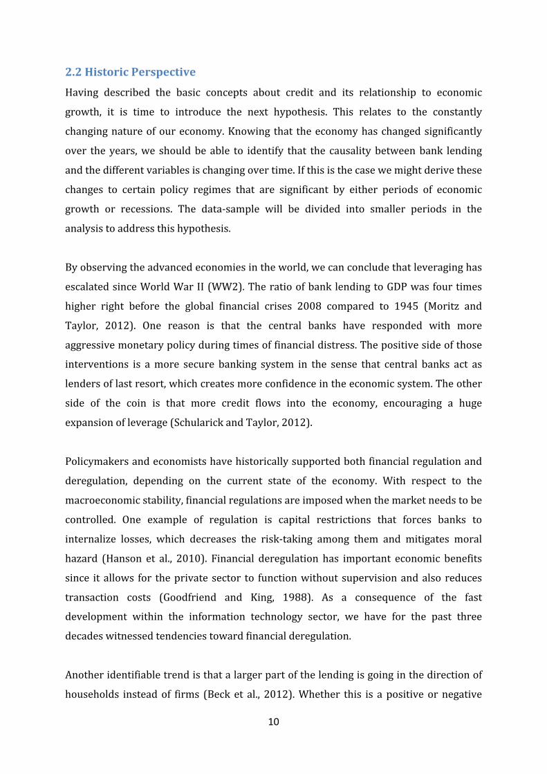
(Hansson and Lindgren, 1989). Figure 1 presents the mortgage share of total bank

lending between 1870 and 1968. Unfortunately this data was presented only up until

this date, but research from Jordá et al. (2014) shows that the increasing trend is intact.

Between 1960 and 2010 the total bank lending in Sweden increased by a factor of 0.8,

where 0.5 of these were mortgage lending and 0.3 were non-‐mortgage lending.

14

Figure 1

Source: See Appendix A

From the 1950’s and onwards the competition among the financial institutions got

tougher. Mergers happened more frequently which resulted in a few, very powerful,

banks. As of today, the Swedish banking system is highly concentrated to the four largest

banks; Handelsbanken, Nordea, SEB and Swedbank whom together stands for roughly

75 % of both borrowing and lending, meaning they have a fundamental role in the

function of the financial system (The Riksbank, 2014).

A process of deregulation of the commercial banks and the capital markets started

approximately 1985, which meant that the banks could widen their business models and

find more opportunities to increase their profits. The Riksbank did no longer control the

maximum amounts of lending, which caused the demand and supply of credit to rise

steeply (Jonung, 2000). This rapid increasing financial activity was soon replaced by a

more negative environment for the banks, when large capital outflows and high interest

rates, among other things, caused a banking crisis in beginning of the 90’s. The crisis

peaked when Sweden was forced to leave the fixed exchange rate regime, resulting in

severe consequences like high rates of unemployment, a price fall on the real estate

0

0,1

0,2

0,3

0,4

0,5

0,6

0,7

1870 1880 1890 1900 1910 1920 1930 1940 1950 1960

Mortgage Share of Total Bank Lending

15

market, lower industry output and increased government deficit (ibid). From 1992 and

onwards, Sweden has applied a floating exchange rate system.

Magnusson (2000) called the structural change that took place after the crisis by “the

third industrial revolution” and stated that the core in this revolution was the new

information-‐ and communication technology available, further increased globalization

and better efficiency in form of increased factor productivity. This revolution was not

something unique for Sweden, but such a significant event like a banking crisis seems to

have become a defining moment in the history. Furthermore, The Riksbank got more

responsibility for the financial stability instead of the government after the deregulation.

One part of the change was that The Riksbank decided to establish an inflation target at

2 per cent annually in 1993 (The Riksbank, 1993). During this regime the financial

stability was reckoned to be solid and the real economy in Sweden performed well until

the crisis 2008. One reason for this fine period of economic growth was credited to the

stable monetary policy conducted and the general understanding was that there were

efficient ways and tools to encounter financial crises (Ingves, 2013). With result in hand,

the recent crisis showed us that the tools (mainly the repo-‐rate) were not as good as

predicted, or rather that the tools were insufficient to adapt to the changes in the

financial system. The Swedish economist Lars Heikensten, former governor of the

Riksbank and member of the Swedish Finance Ministry, doubts the capability of the

Riksbank to pursue the primary goal of low and stable inflation and at the same time

make sure that we have a secure and stable payment system, i.e. work for financial

stability (Heikensten, 2014). The present Governor of the Riksbank, Stefan Ingves,

confirms that he is worried about the current situation. He states that the greatest fear

right now is the accumulation of debt with simultaneous rapid price increases on real

estate that is ongoing. The severe consequences from this cannot be neglected, with the

U.S. housing market as a recent example (Ingves, 2013). The below graph presents a

price index for residential property in Sweden, indicating that the prices grew roughly at

the same pace as the average price level until 1990, whereas for the latest 25 years the

prices have spiked. The two series has been normalized to 100 for 1875 and for 1957.

16

Figure 2

Source: See Appendix C

The implications of rapid increases in residential property prices and credit have been

stressed by Jordá et al. (2014). They claim that growing levels of mortgages creates

financial fragility and problems for the macroeconomic policies. To the contrary,

Finocchario et al. (2011) argues that it has historically been difficult to predict asset

price bubbles and that other factors have strong influence of the house-‐prices in

Sweden, for example a strong regulated market for residential property, limited market

for renting and the allocation of debt. Furthermore, there is evidence that the price

increases of residential property in Sweden mainly emerges from the biggest cities

(Englund, 2011), hence the whole picture will not be included here since this thesis is

limited to the prices in Stockholm and Gothenburg. Another important factor that drives

the prices upwards is that the demand for housing exceeds the supply in these cities. In a

report by Englén et al. (2014) it is concluded that the immigration and the high birth

rate are the reasons for the growing population in the capitol.

0

50

100

150

200

250

300

350

400

1875

1879

1883

1887

1891

1895

1899

1903

1907

1911

1915

1919

1923

1927

1931

1935

1939

1943

1947

1951

1955

1959

1963

1967

1971

1975

1979

1983

1987

1991

1995

1999

2003

2007

2011

Price Index for Residential Property

Price index residental property, Gothenburg

Price index residental property, Stockholm

17

To justify a continued examination regarding bank lending and economic growth in

Sweden, the below figure illustrates the ratio between bank lending and total GDP from

1870 to 2014, indicating an increasing trend over the series.

Figure 3

Source: See Appendix A and B

It is now motivated to perform the statistical tests to find an answer to the two

hypotheses stated in earlier chapter. Next section will firstly describe and motivate the

data and the econometric model followed by an analytical part where the results will be

presented.

0

0,2

0,4

0,6

0,8

1

1,2

1,4

1,6

1,8

2

1880

1884

1888

1892

1896

1900

1904

1908

1912

1916

1920

1924

1928

1932

1936

1940

1944

1948

1952

1956

1960

1964

1968

1972

1976

1980

1984

1988

1992

1996

2000

2004

2008

2012

Ratio Between Total Bank Lending and GDP

18

4. Empirical Analysis

4.1 Data

Creating a long and consistent time series of bank lending in Sweden is one of the

contributions of this thesis. It was time-‐consuming to find data from various sources and

adjust to changes in definitions over the sample period. Furthermore, a major part of

SCB’s data set was recently digitalized and therefore not many similar studies have had

access to this material so far (SCB, 2015a). Structural changes in both the banking

sector, in terms of mergers and new startups, and bank’s balance sheets results in

difficulties of accurate measuring total bank lending. The number of participants on the

financial markets has also grown extensively during the sample period. Even though

banks still are the most important and biggest ones when it comes to credit, new

institutions as investment banks, pension funds, insurance companies and mutual funds

now also play substantial roles (IMF, 2015). All the commercial banks, savings banks

and co-‐operative banks are included in the measure and other financial intermediaries

and the central bank are excluded. The data on bank lending is used from the official

bureau of statistics in Sweden (SCB, 2015d) and from Bank of International Settlements

(BIS, 2015). An inflation-‐index created by Edvinsson and Söderberg (2010) and SCB

(2015b) is used to convert all values from nominal to real ones. For more details

regarding the data on bank lending, see Appendix A.

As for real economic activity, the following variables were collected: Swedish data of

labor productivity (represented by GDP per employee per year), capital stock, total

factor productivity (TFP) and GDP per capita in the U.S.. as a control variable. Other

papers that measures real economic activity had similar choices of variables (N.G

Andersson et al., 2013 and Bordo and Haubrich, 2009). However, given that this thesis

has a long time-‐span, the measurement of GDP per employee per year and TFP are

different from those that examine shorter time periods. Choosing GDP per employee per

year is a more reasonable measurement of economic activity than GDP per capita, as it

captures for at least two important facts. These are that people worked more hours per

day in the past and that women gradually have been integrated in the workforce. As for

TFP, Bengtsson (2012) argues that the labor’s share of income varies more than just

over the business cycle and that it would be inappropriate to use the same number over

19

the whole series. The argument is that the production of goods and services is more

capital intensive rather than labor intensive today. Using a variable measure of labor’s

share of income will be more justifiable than having a constant value. Further details on

this data are available in Appendix B.

The real assets are represented by price index for residential property in Stockholm and

Gothenburg and a house price index for the U.S. as a control variable. We are currently

seeing fast escalation in these indices in Sweden, especially in the major cities.

According to the common index for housing, HOXSWE, the index has doubled since the

measurement began in 2005 (Nasdaq Nordic, 2015).

However, due to this short period of time that HOXSWE provides, data from Bohlin

(2014) and Blöndal et al. (2014) are used, which stretches from 1875 to 2012. The index

is constructed from information on sale-‐prices as well as tax assessment values and the

method is called the “sales price ratio method”. As is pointed out by the authors,

measuring residential property index is rather complicated and the specification is very

different compared to stock indices. One example is that the description of securities

does not change over time, while residential properties are heterogeneous and unique

objects with different quality and they are also traded more infrequently.

The last set of data is an annual stock index in Sweden as a representation for the

financial assets and an index for Standard & Poors (S&P) as a control variable.

Waldenström (2014) provides the entire Swedish series and Williamson (2015) the one

for S&P. There are two main reasons to include financial assets in the model; the first

one is that a lot of credit naturally moves in the direction of financial assets and secondly

financial assets are less sticky than the real economy and real assets, making it

interesting to see how this might impact the results. More details on the data of real and

financial assets can be found in Appendix C.

4.2 Motivation of Sample Periods

To examine whether the results are robust or if the interpretation is different depending

on which period is analyzed, the data is divided into sub-‐samples. This will provide a

hint if the relation between the variables has changed during different policy regimes in

20

Sweden. Selecting the subsamples will be based on historic events that had significant

effects on the economy and to some extent the availability of variables. For example,

Shiller’s index of housing data in the U.S. did not start until 1891 and in 1957 an average

of house-‐ and apartment prices have been used, making it more reasonable to start at

that specific year rather than 1947 (also described in Appendix C).

The start of WW1 combined with tighter regulations of the banking sector marks the

first period. Secondly, the inter-‐war period is analyzed. The end of WW2 brought new

economic structures including greater importance of active macroeconomic policies,

additional bank supervision and a more explicit role of the central banks as “lenders of

last resorts” (Schularick and M .Taylor, 2012) and hence marks the beginning of the

third period. Lastly, the financial deregulation in Sweden during the 1980’s will be the

last break of the series. The table below lists the sub-‐samples used for the different

variables.

Table 1. Regressions and sample periods.

Regression of Period 1 Period 2 Period 3 Period 4

Real Economic Activity

vs. Bank Lending 1870-‐1912 1919-‐1939 1947-‐1985 1986-‐2010

Real Assets vs. Bank

Lending 1891-‐1912 1919-‐1939 1958-‐1985 1986-‐2012

Financial Assets vs.

Bank Lending 1871-‐1912 1919-‐1939 1947-‐1985 1986-‐2012

Furthermore, regressions on the entire sample period are made as well. In that case,

dummies have been included for 1914-‐1918 and 1939-‐1945 to avoid the large effects

that the two World Wars brought.

The selection of time periods has support in the literature. Moritz and M. Taylor (2012)

made a similar study for advanced economies and found a stable relationship between

economic growth and volume of credit between 1870 and 1944 except from the Great

Depression. During the post-‐war period however, the credit grew more rapidly once the

recovery was over, especially after the financial deregulation.

21

4.3 The Model

The data-‐set on the four variables are used to set up a VAR-‐model and test for non-‐

Granger Causality. It is important to emphasize that the existence of unit roots or co-‐

integrating relations themselves are not the goal of this econometrical model, but rather

to look at the causality between the variables (Toda and Yamamoto, 1995). The non-‐

Granger causality test shows whether one time series variable’s future values are better

predicted with the history of only that variable itself, or if more explanatory power can

be obtained when using another variable’s history also. In our case, we are interested in

the causality between bank lending and the other variables and whether the

relationships have changed over the sub-‐samples.

Totally 15 estimations were made for tests in levels, four for each period of real

economic activity, real assets and financial assets. In addition, one test was made for the

whole sample period, except for the excluded periods of war. The same procedure was

repeated for testing the short-‐run effect, by using the first difference.

4.3.1 Test in First Difference

A VAR-‐model is estimated to test for the short-‐run associations among the variables. The

first difference is used in the first three tests.

𝐵𝐿! = 𝑎! + 𝑎!𝐵𝐿!!! +⋯+ 𝑎!𝐵𝐿!!! + 𝑎!𝑅𝐸!!! + 𝑎!𝑋!!! + 𝜀! (1)

𝐵𝐿! = 𝑎! + 𝑎!𝐵𝐿!!! +⋯+ 𝑎!𝐵𝐿!!! + 𝑎!𝑅𝐴!!! + 𝑎!𝑋!!! + 𝜀! (2)

𝐵𝐿! = 𝑎! + 𝑎!𝐵𝐿!!! +⋯+ 𝑎!𝐵𝐿!!! + 𝑎!𝐹𝐸!!! + 𝑎!𝑋!!! + 𝜀! (3)

BL represents bank lending, RE is real economic activity, RA is real assets and FA is

financial assets. X is the control variable and is represented by U.S. data on GDP per

capita (1), real house price index (2) and real stock index (3), to see if bank lending

could be affected by something else than the variables chosen. 𝜀! represents the error

term. To have U.S. data as a control for misspecification of our model is reasonable since

we assume that the U.S. economy affects the Swedish, but the causality should not be

true for the reverse case. If we do not find significance for our control variable in a

particular model, then the results obtained are stronger.

22

If the coefficient 𝑎 equals 0, then the null-‐hypothesis of non-‐Granger causality is rejected

and hence the explanatory variable does help to explain the history of the dependent

variable. Lag length of my non-‐Granger causality is set to 2 since we are dealing with

annual data. Tests were performed with both one and two lags and the results were

roughly the same.

4.3.2 Test in Levels

Toda and Yamamoto (1995) provide a technique to perform a non-‐Granger causality

test for long-‐run associations. The equations are rather similar to the previous section,

but one additional lag has been included to control for non-‐stationarity. The strength of

this technique is that we do not have to mind the order of integration or the co-‐

integration when we are running the regressions.

𝐵𝐿! = 𝑎! + 𝑎!𝐵𝐿!!! +⋯+ 𝑎!𝐵𝐿!!! + 𝑎!𝐵𝐿!!!!! + 𝑎!𝑅𝐸!!! + 𝑎!𝑅𝐸!!!!! + 𝑎!𝑋!!! +

𝑎!𝑋!!!!! + 𝜀! (4) 𝐵𝐿! = 𝑎! + 𝑎!𝐵𝐿!!! +⋯+ 𝑎!𝐵𝐿!!! + 𝑎!𝐵𝐿!!!!! + 𝑎!𝑅𝐴!!! + 𝑎!𝑅𝐴!!!!! + 𝑎!𝑋!!! +

𝑎!𝑋!!!!! + 𝜀! (5) 𝐵𝐿! = 𝑎! + 𝑎!𝐵𝐿!!! +⋯+ 𝑎!𝐵𝐿!!! + 𝑎!𝐵𝐿!!!!! + 𝑎!𝐹𝐸!!! + 𝑎!𝐹𝐸!!!!! + 𝑎!𝑋!!! +

𝑎!𝑋!!!!! + 𝜀! (6)

The following variables are linearized by taking logarithms of the initial values: Bank

loans, GDP per employee per hour, U.S. GDP per capita, capital stock, real price stock

index in Sweden and Average S&P common stock index. This is to avoid exponentially

growing series.

23

5. Results and Discussion This section aims at evaluating the hypotheses by presenting and analyzing the results

from the tests. Testing the first differences reveals the short-‐run causality while the tests

in levels are related to the long-‐run. Finally, a further discussion is held regarding some

problems related to the data and the model.

5.1 Short-‐Run

Tests for non-‐Granger causality between bank lending and the real economy lack

significant results over the short-‐run. A more important result is that real assets

Granger-‐causes bank lending in the fourth period and that the reverse is not true,

indicating a unidirectional relationship. It suggests that we have a situation where prices

on residential property are driving bank lending to some extent in Sweden. This is

opposite of what Mian and Sufi (2014) concluded, which was that the causality ran the

other way around during the credit boom in the U.S. in the early 2000’s. The control

variable for the regression, home prices in the U.S., is insignificant which provides

strength to this result.

Table 2: Results of the non-‐Granger causality test for first difference.

Granger causality Period 1

RE: 1870-‐1912 RA: 1891-‐1912 FA: 1871-‐1912

Period 2 RE: 1919-‐1939 RA: 1919-‐1939 FA: 1919-‐1939

Period 3 RE 1947-‐1985 RA: 1958-‐1985 FA: 1947-‐1985

Period 4 RE: 1986-‐2010 RA: 1986-‐2012 FA: 1986-‐2012

Whole sample

Granger causality between

BL and RE -‐ BLßRE*! -‐ -‐ -‐


BL and RA -‐ BLßRA*! -‐ BLßRA* -‐


BL and FA -‐ BLßàFE** BLàFE*! -‐ -‐

Note: “*” and “**” Denotes significance at a 5% level and at a 10% level respectively. “ßà”denotes causality both ways,

“ß” one way and “-‐“ no causality at all. “!” indicates that the control variable is significant.

Source: See Data-‐section

It is interesting that this result emerges in a period that was characterized by increased

leveraging among the households. This does somewhat identify the source of the

problem with increased bank lending; the current house-‐ and apartment prices in the

biggest cities forces citizens to borrow more to afford living. With this result in mind,

24

the development of the prices on the housing market may be something that the

authorities should put more emphasis on. The Riksbank state that the most crucial

threat against the financial stability in Sweden is the amount of debt accumulated by the

households, where a major part consists of mortgages (The Riksbank, 2015c).

This creates a conflict for the Riksbank and highlights the consequences of monetary

policy. Their mean of controlling the inflation is through the short term interest rate.

Suppose they want to lower the interest rate in order to boost inflation and in turn the

demand for goods and services. What this also implicates is an increasing demand for

credit, since the consumers gets more utility of borrowing money than saving due to the

low interest rates that prevails. If the households expect the interest rate to remain low

in combination with an economy that grows over a longer period, they will borrow more

money to invest even more in housing. Gan (2010) suggest that the major part of

household’s wealth comes from houses rather than consumption. This indicates that the

attempt of the Riksbank to boost the inflation in fact more likely feeds the real estate

market. This spiral will inevitably create an asset bubble, which upon bursting will affect

the whole economy severely, having in mind what happened in the U.S. during 2008.

This summarizes the challenge for the Riksbank; it is difficult to fight low inflation and

simultaneously control the housing prices when the interest rates are at these low

levels.

From reading Table 2 we can see that the inter-‐war period provides significance for all

the estimations in the short-‐run, which is something that has to be interpreted with

care. It is not very likely that the model perfectly describes the relationship between

bank lending and the other variables. In addition to this, the number of observations is

too few to draw any meaningful conclusions during this period. In period three bank

lending is Granger causing financial assets, but the control variable is also significant for

this regression.

Due to the lack of results in the short-‐run it is hard to draw any further conclusions and

answer the initial state hypotheses. In order to investigate the matter in more detail, we

will move on to the long-‐run.

25

5.2 Long-‐Run

The results for the long-‐run tests are presented in Table 3 below.

Table 3: Results of the non-‐Granger causality test for level data.

Granger causality

Period 1 RE: 1870-‐1912 RA: 1891-‐1912 FA: 1871-‐1912

Period 2 RE: 1919-‐1939 RA: 1919-‐1939 FA: 1919-‐1939

Period 3 RE: 1947-‐1985 RA: 1958-‐1985 FA: 1947-‐1985

Period 4 RE: 1986-‐2010 RA: 1986-‐2012 FA: 1986-‐2012

Whole sample

Granger causality

between BL and RE -‐ BLßRE*! BLàRE** BLßRE* BLàRE*

Granger causality

between BL and RA BLàRA* BLßRA*! BLàRA* BLßRA** -‐

Granger causality

between BL and FE -‐ BLßàFE*! BLàFE*! -‐ -‐

Note: “*” and “**” Denotes significance at a 5% level and at a 10% level respectively. “ßà”denotes causality both

ways, “ß” one way and “-‐“ no causality at all. “!” indicates that the control variable is significant.

Source: See Data-‐section

The Granger causality tests between bank lending and the real economy provides

somewhat ambiguous and non-‐robust results. In the third period and for the whole

sample, the history of bank lending can help predict the future values of the real

economy, but the opposite is true during the fourth period. What is worth mentioning is

that the fourth period only had 22 observations compared to the third period and the

whole sample, which had 36 and 128 observations respectively. Thus, more credibility is

given to the stronger results where more observations are included. To some extent, this

does confirm the second hypothesis, that the effect of bank lending has changed over

time and that the deregulation in the 1980’s coincides with this result. Period 2 was also

characterized by deregulation and even though the control variable is significant for all

tests in this period, it confirms the causality that occurred in the fourth period.

The regression between bank lending and the real economy is the only full sample test

that provides significance, both for the short and the long-‐run and it is also significant at

a 5 % level. A closer look at this result tells us that it is the factor productivity that is

Granger-‐caused by bank lending in a unidirectional way. What this implies is that when

larger amounts of credit are given from banks to firms, the production of goods and

26

services has become more effective through investments in technology and human

capital. We did have the same causality in the third period as for the whole sample and

Sweden during that period was characterized by a strong industry that occupied a large

part of the workforce. It follows quite naturally that this outcome emerges in the long-‐

run and not in the short-‐run tests, because investments in the production takes time

before it can yield any improvement. Organizations, capital, knowledge and other inputs

in the production process have to be rearranged in order to adapt to new and more

efficient technology (Magnusson, 2000).

To further relate this to theory, Friedman and J. Schwartz (1963) pointed out that credit

booms are a leading indicator over the real economy, which seems to be true for Sweden

during a major part of the 2000th century. Prior to the financial crisis in the early 1990’s,

bank lending was a good predictor of both the real economy and real assets. In the

financial climate that prevailed during the third period, consumers and firms had few

incentives to save money due to the high rates of inflation. Figure 4 depicts the inflation

rate over the sample period.

Figure 4

Source: Edvinsson and Söderberg (2010) and SCB (2015).

The situation promoted borrowing and in combination with strong capital controls

imposed by the government, large amounts of credit were held within the borders.

When suddenly the capital controls where released and credit was allowed to float

freely, the fixed exchange rate regime broke down and a financial crisis was triggered.

-‐30

-‐20

-‐10

0

10

20

30

40

50

60

1870

1875

1880

1885

1890

1895

1900

1905

1910

1915

1920

1925

1930

1935

1940

1945

1950

1955

1960

1965

1970

1975

1980

1985

1990

1995

2000

2005

2010

Rate of Infla7on %

27

Moving on to the next result we can see that bank lending is Granger-‐causing house-‐

prices in both Stockholm and Gothenburg during the third period and that the control

variable is significant for Stockholm. The causality between bank lending and real assets

thereby seems to be similar to the relationship between bank lending and the real

economy, which contradicts the hypothesis that bank lending affects the variables

differently. Hansson and Lindgren (1989) identified that the commercial banks shifted

focus from investments in the industry to the housing market around the 1950’s. The

timing coincides with the result of the estimation made, that bank lending seems to have

been a driving factor for the real assets in Stockholm and Gothenburg. The result in the

fourth period is contradictory to the one in the third period, but only at a 10 %

significance level. Still it indicates that we have the same result in the fourth period for

both the short-‐run and the long-‐run for real assets.

5.3 Data Issues

The first thing to notice is that for some of the estimations, the different representations

of the variables seem to explain each other. For example, GDP per employee per year

explains the future values of factor productivity in the fourth period quite well. Both

belonging to the group of real economy, it means that one explanatory variable Granger-‐

causes another. A similar result is found for the asset prices in Stockholm and

Gothenburg for some periods and the correlation between those two measures is high.

In addition to this, the results are more significant for the long-‐run and later periods

compared to the short-‐run and earlier periods. It is reasonable to assume that the

theories and choices of data better fits the economic environment of today than in the

beginning of the sample. As the recent history of Sweden has told us, the country has

gone through several structural changes in recent times that have affected the economy.

This means that the purpose of bank lending is different today and confirms our

expectation regarding the second hypothesis; the effect of bank lending has changed

over time. Significant results in the first period are missing, except from that the real

asset prices in Stockholm were Granger-‐caused by bank lending in the long-‐run test. If

we would have got more interpretable results in the first period, we could have used

these to really compare to later periods and achieve a stronger confirmation of the

hypothesis.

28

The first hypothesis relates to the effects of credit on the different economic variables.

For the short term, no results indicate that bank lending has affected the variables

differently over the same estimation window. For the long term, both period three and

four showed similar ways of causation for the estimations. Bank lending was a good

predictor of the economy in the third period and vice versa was true for the fourth

period (except for financial assets in the latter case).

Further, it can be argued that the sample periods chosen are too small. Especially period

two and four ended up with very few observations, below 30 which is a critical level.

The alternative was to choose fewer time periods to get rid of this problem but in that

case, it would be harder to answer the question at hand and the tests would be more

similar to the one conducted on the whole sample. The goal was to determine structural

shifts that could work as natural motivations for the sample periods chosen. In addition

to this, another weakness with this econometric technique is that the non-‐Granger

causality test is sensitive to the specification of the model. If relevant variables are

excluded from the model and hence not accounted for, then the empirical evidence is

fragile (Alimi and Ofonyelu, 2013). The lack of result in the first period could be a sign of

misspecification.

We did not found supporting evidence to the theory about price stickiness, which could

be explained by the lack of results when testing the relationship between bank lending

and financial assets. Financial assets were expected to be affected faster by changes in

bank lending after a structural change, for example a period of deregulation, than the

real assets and the real economy. The few significant results that were observed are

weak due to that the control variable was significant as well. It could be that the stock

market is not representing financial assets well enough and that additional variables

would have solved this problem by indicating some sort of causing relationship.

Anyhow, the ongoing financialization is still relevant to discuss in the light of the future

economic growth in Sweden. It gives many possibilities to find financing abroad when

investments are about to be made, but there are also dangers with the high transparency

and globalization. Giannetti (2014) stresses one negative fact, which is that both

investors and banks today are affected by the “flight home” effect, which means that in

times of domestic financial distress, they generally cut of activity abroad to decrease

risks and instead move these funds to domestic markets. The consequence is that

29

financial shocks and credit cycles are transmitted from the original country to the

international markets more than what would be necessary.

6. Concluding Remarks Despite the fact that the results from the non-‐Granger causality tests are quite

insignificant, we can still draw some meaningful conclusions. One of the main findings in

this thesis is that the effect of bank lending on a number of economic performance

measures has changed over time, corresponding to the fact that the role of credit has

changed as well. It could not be determined how bank lending specifically affected the

different variables, which meant that this hypothesis was not supported by the results. It

can be concluded that the economic environment is very complex and that additional

variables could have added more significance to the results. The non-‐Granger causality

tests for the short-‐run provided overall insignificant results, except that real assets

Granger-‐caused bank lending in the fourth period.

Bank lending, asset prices and prices on the stock market have surged since the early

1990’s, apart from a few exceptions during crises. One factor behind the current

financial climate is the expansionary monetary policy driven by The Riksbank in pursuit

of increasing the rate of inflation. It has clearly contributed to that the ratio between

bank lending and GDP has increased over the last two decades. Some argues that The

Riksbank does not have the tools to ensure both financial stability and work for an

inflation target. Representatives from Finansinspektionen and the Swedish Government

have expressed anxiety over the financial stability and the fact that more people today

are dependent on credit to survive (Svenska Dagbladet, 2015). This supports the fact

that this is a critical issue that deserves a lot of attention in the current debate.

Another finding in this thesis is that the increased leveraging among households in

Sweden is one of the greatest future concerns. Economists argue that a substantial part

of this leveraging is connected to higher prices on real estate in the biggest cities. This

challenge was to be addressed by the new mortgage requirement presented by

Finansinspektionen during the summer of 2015, which did not happen after all, because

the court in Jönköping claimed that the change was not supported by the law

(Finansinspektionen, 2015).

30

A suggestion for further research within the area of credit and economic growth in

Sweden would be to find better and additional proxies for the financial economy, since

those results were least significant. The financial sector will certainly gain more

importance in the aspect of the increased globalization and deregulation that we are

seeing. To incorporate more than just the asset prices in Stockholm and Gothenburg

would also be interesting and provide a more general picture over the real estate

market. By doing so, a different view of the relationship between bank lending and real

assets might be seen.

This thesis did not aim to predict when the next financial crisis in Sweden will occur;

such a task is very difficult even for the most initiated economists. The goal was rather

to describe the purpose and history of bank lending in Sweden from a long-‐run

perspective and to see if the causality relationships changed during different policy

regimes.

31

7. References

Alimi, Santos R. and Ofonyelu, Chris C. 2013. “Toda-‐Yamamoto causality test between

money market interest rate and expected inflation: The Fisher Hypothesis revisted”

European Scientific Journal. March 2013, Vol 9, No. 7.

Andersson. N.G., Fredrik, Burzynska, Katarzyna and Opper, Sonja. 2013. “Lending for

Growth? An Analysis of State-‐Owned Banks in China” Lund University, Department of

Economics, Working Paper 2013:19.

Bank for International Settlements. 2015. “Long series on credit to the private non-‐

financial sector” Available at: http://www.bis.org/statistics/credtopriv.html

Retrieved 2015-‐05-‐22.

Beck, Thorsten, Rioja, Felix K., Büyükkarabacak, Berrak and Valev, Neven T. 2012.

”Who Gets the Credit? And Does It Matter? Household vs. Firm Lending Across

Countries” The B.E Journal of Macroeconomics, Vol. 12, Issue 1, Article 2.

Bengtsson, Erik. 2012. “Labor’s Share in Sweden, 1850-‐2000” Gothenburg University,

Version 1.1.

Blöndal, Sölvi, Edvinsson, Rodney and Söderberg, Johan. 2014. “A price index for

residential property in Stockholm, 1875–2011” House Prices, Stock Returns, National

Accounts, and the Riksbank Balance Sheet, 1620–2012, Vol. 2, Ch. 3.

Bohlin, Jan. 2014. “A price index for residential property in Göteborg, 1875–2010”

House Prices, Stock Returns, National Accounts, and the Riksbank Balance Sheet, 1620–

2012, Vol. 2, Ch. 2.

Carvalho, Carlos. 2006. ”Heterogeneity in Price Stickiness and the Real Effects of

Monetary Shocks” Frontiers of Macroeconomics, Vol. 2, Issue.1, Article 1.

32

Claessens, Stijn, Kose, Ayhan M., and E. Terrones, Marco. 2008. ”What Happens During

Recessions, Crunches and Busts?” IMF Working Paper 2008, No. 274.

Cobb, Charles W & Douglas, Paul H. 1928. ”A Theory of Production” The American

Economic Review, Vol. 18, No. 1, pp. 139-‐165.

Bordo, Micheal D. and Haubrich, Joseph G. 2009. ”Credit Crises, Money and Contractions:

An Historical View”. NBER Working Paper Series, Working Paper No. 15389.

De Gregorio, Jose and Guidotti, Pablo E. 1995. “Financial development and economic

growth” International Monetary Fund, Vol. 23, Issue 3, pp.433-‐448.

De Gregorio, Jose. 1996. “Borrowing Constraints, Human Capital Accumulation, and

Growth” Journal of Monetary Economics, Vol. 37, Issue. 1, pp. 49-‐71.

Edvinsson, Rodney. 2015. ”Historical national accounts for Sweden 1800-‐2000” Almqvist

& Wiksell International; Stockholm, Version 1.

Edvinsson, Rodney and Söderberg, Johan. 2010. “The evolution of Swedish consumer

prices, 1290–2008” Historical Monetary and Financial Statistics for Sweden: Exchange

Rates, Prices, and Wages, 1277-‐2008, Chapter 8.

Englén, Tore, Hasselgren, Björn, Långsved, Göran and Weiss, Lennart. 2014.

”Stockholmsregionens utmaningar – Nu brådskar nya lösningar”. Stockholms

Handelskammare, 2014, No. 7.

Englund, Peter. 2011. ”Swedish house prices in an international perspective” The

Riksbank’s inquiry into the risks in the Swedish housing market, Chapter 1, pp. 23-‐65.

Finansinspektionen. 2015. “FI går inte vidare med amorteringskravet” Available at:

http://fi.se/Press/Pressmeddelanden/Listan/FI-‐gar-‐inte-‐vidare-‐med-‐

amorteringskravet/

Retrieved 2015-‐08-‐11.

33

Finocchiaro, Daria, Nilsson, Christian, Nyberg Dan and Soultanaeva, Albina. 2011. ”The

household indebtedness, house prices and the macroeconomy: a review of the

literature” The Riksbank’s inquiry into the risks in the Swedish housing market, Chapter

2, pp. 109-‐134.

Friedman, Milton and J.Schwartz, Anna. 1963. “Money and Business Cycles” Review of

Economics and Statistics 45, No. 1, part. 1, pp. 32-‐64, The MIT Press.

Gan, Jie. 2010. “Housing Wealth and Consumption Growth: Evidence from a Large Panel

of Households” Hong Kong University of Science and Technology.

Giannetti, Mariassunta. 2014. ”Finanskriser och den finansiella integrationens kollaps”.

Ekonomisk debatt, 2014, No. 7.

Goodfriend, Marvin and King, Robert G. 1988. “Financial Deregulation, Monetary Policy,

and Central Banking” Federal Reserve Bank of Richmond, Working paper No. 88-‐1.

Hanson, Samuel G., Kashyap, Anil and Stein, Jeremy C. 2010. “A Macroprudential

Approach to Financial Regulation” Chicago Booth Research Paper, Working Paper No. 10-‐

29.

Hansson, Pontus and Jonung, Lars. 1997. ”Finance and economic growth: the case of

Sweden 1834-‐1991” Research in Economics, Vol. 51, Issue 3, pp. 275-‐301.

Heikensten, Lars. 2014. ”Inflationsmålspolitiken, den finansiella stabiliteten och

Riksbankens direktion” Summary of Oral presentation in ”Nationalekonomiska

Föreningens förhandlingar”, 2013-‐11-‐26.

Huberman, Michael and Minns, Chris. 2007. ”The times they are not changin’: Days and

hours of work in Old and New Worlds, 1870–2000” Explorations in Economic History, No.

44, pp. 538–567.

34

Ingves, Stefan. 2013. “Central bank policies – the way forward after the crisis”. Speech

at Royal Bank of Scotland 2013-‐10-‐04.

IMF. 2015. ”Rethinking Financial Deepening: Stability and Growth in Emerging Markets”

Available at: https://www.imf.org/external/pubs/cat/longres.aspx?sk=42868.0

Retrieved 2015-‐05-‐16.

Jappelli, Tullio and Pagano, Marco. 1994. “Saving, Growth, and Liquidity Constraints”

Quarterly Journal of Economics, No. 106, pp. 83-‐109.

Johnston, Louis and Williamson, Samuel H. 2015. "What Was the U.S.. GDP Then?"

Available at: http://www.measuringworth.com/usgdp/

Retrieved 2015-‐05-‐04.

Jonung, Lars. 2000. ”Från guldmyntfot till inflationsmål – svensk stabiliseringspolitik

under det 20:e seklet” Ekonomisk Debatt, 2000, No. 1.

Jonung, Lars. 2015. ”Trettio år på Vägen till ett stabilare Sverige. Var står vi nu?” Lund

University, Department of Economics, Policy paper 2015, No. 1.

Jordá, Òscar, Schularick, Moritz and Taylor, Alan M. 2014. ”The Great Mortgaging:

Housing Finance, Crises, and Business Cycles” NBER Working Paper No. 20501.

Jordá, Òscar, Schularick, Moritz and Taylor, Alan M. 2015. ”Mortgaging the Future”

FRBSF Economic Letter 2015-‐09.

Josheski, Dushko, Lazarov, Darko and Koetski, Cane. 2011. “Cobb-‐Douglas Production

Function Revisited, VAR and VECM Analysis and a Note on Fischer/Cobb-‐Douglass

Paradox” Available at: http://papers.ssrn.com/sol3/papers.cfm?abstract_id=1931117

Retrieved: 2015-‐04-‐26

King, Robert G. and Levine, Ross. 1993. “Finance and Growth: Schumpeter Might be

Right” The Quarterly Journal of Economics, Vol. 108, No. 3, pp. 717-‐737.

35

Kuznets, Simon. 1940. ”Schumpeter's Business Cycles” The American Economic Review,

Vol. 30, No. 2, Part 1, pp. 257-‐271.

Larsson, Mats and Lindgren, Håkan. 1989. ”Risktagandets gränser, utvecklingen av det

svenska bankväsendet 1850-‐1980” Uppsala Papers in Economic History, 1989, No. 6.

Levine, Ross and Zervos, Sara. 1998. “Stock Markets, Banks, and Economic Growth” The

American Economic Review, Vol. 88, No. 3, pp. 537-‐558.

Maddison, Angus. 1994. ”Standardised Estimates of Fixed Capital Stock: A Six Country

Comparison” Groningen Growth and Development Centre, University of Groningen, No.

199409.

Magnusson, Lars. 2000. “Vad är egentligen det nya i den nya ekonomin?”, Ekonomisk

debatt, 2000, No. 6.

Mian, Atif and Sufi, Amir. 2014. “House of Debt: How They (and You) Caused the Great

Recession, and How We Can Prevent It from Happening Again”. The University of

Chicago Press.

Nasdaq Nordic. 2015. “HOXSWE index” Available at:

http://www.nasdaqomxnordic.com/index/historiska_kurser?Instrument=SE00038488

52

Retrieved 2015-‐05-‐27.

OECD StatExtracts. 2015. “Average annual wages”

Available at: https://stats.oecd.org/Index.aspx?DataSetCode=AV_AN_WAGE#

Retrieved 2015-‐05-‐14

Pereira, Maria da Conceição Costa. 2006. “The effects of households’ and firms’

borrowing constraints on economic growth” Portuguese Economic Journal, 2008, Vol. 7,

Issue 1, pp 1-‐16.

36

Reinhart, Carmen and Rogoff, Kenneth. 2010. “Debt and Growth Revisited” Munich

Personal RePEc Archive MPRA Paper No. 24376.

Reinhart, Carmen M., Reinhart, Vincent R. and Rogoff, Kenneth. 2012. “Public Debt

Overhangs: Advanced-‐Economy Episodes Since 1800” Journal of Economic Perspectives

Vol. 26, No. 3, pp. 69-‐86.

Schön, Lennart and Krantz, Olle. 2012. ”Swedish Historical National Accounts 1560-‐

2010” Lund Papers in Economic History 123, Lund University.

SCB. 2015a. “Om digitaliseringen” Available at: http://www.scb.se/sv_/Hitta-‐

statistik/Historisk-‐statistik/Om-‐digitaliseringen/ Retrieved 2015-‐04-‐15.

SCB. 2015b. “Inflation i Sverige 1831-‐2014” Available at: http://www.scb.se/sv_/Hitta-‐

statistik/Statistik-‐efter-‐amne/Priser-‐och-‐

konsumtion/Konsumentprisindex/Konsumentprisindex-‐

KPI/33772/33779/Konsumentprisindex-‐KPI/33831/

Retrieved 2015-‐05-‐25.

SCB. 2015c. “Sök historisk statistik” Available at: http://www.scb.se/sv_/Hitta-‐

statistik/Historisk-‐statistik/Sok-‐historisk-‐statistik/

Retrieved 2015-‐04-‐10.

SCB. 2015d. “Sammandrag av enskilda bankernas uppgifter 1866-‐1911” Available at:

http://www.scb.se/sammandragenskildabankernasuppgifter1866-‐1911/

Retrieved 2015-‐05-‐10.

Schularick, Moritz and Taylor, Alan M. 2012. “Credit Booms Gone Bust: Monetary Policy,

Leverage Cycles, and Financial Crises, 1870–2008” American Economic Review, 2012, No.

102(2), pp. 1029-‐1061.

Shiller, Robert. 2015. “U.S. Home Prices 1890-‐Present” Available at:

http://www.econ.yale.edu/~shiller/data.htm

37


Svenska Dagbladet. 2015. ”Amorteringskrav svävade över bankmötet” Available at:

http://www.svd.se/amorteringskrav-‐svavade-‐over-‐bankmotet/om/naringsliv

Retrieved 2015-‐05-‐04.

The Riksbank. 1993. “The Riksbanks target for monetary policy” Press release 1993-‐01-‐

15, No. 5.

The Riksbank. 2014. “ Financial stability report 2014:2” Available at:

http://www.riksbank.se/en/Financial-‐stability/Swedish-‐major-‐banks-‐currently-‐

financially-‐strong/Earlier-‐Financial-‐Stability-‐Reports/2014/Financial-‐stability-‐report-‐

20142/


The Riksbank. 2015a. “The tasks and role of the Riksbank” Available at:

http://www.riksbank.se/en/The-‐Riksbank/The-‐Riksbanks-‐role-‐in-‐the-‐economy/


The Riksbank. 2015b. “Riksbank cuts repo rate to −0.10 per cent, buys government

bonds for SEK 10 billion and is prepared to do more at short notice“Available at:

http://www.riksbank.se/en/Press-‐and-‐published/Press-‐Releases/2015/Riksbank-‐cuts-‐

repo-‐rate-‐to-‐010-‐per-‐cent-‐buys-‐government-‐bonds-‐for-‐SEK-‐10-‐billion/


The Riksbank. 2015c. “Financial stability report 2015:1” Available at:

http://www.riksbank.se/en/Financial-‐stability/Swedish-‐major-‐banks-‐currently-‐

financially-‐strong/Earlier-‐Financial-‐Stability-‐Reports/2015/Financial-‐stability-‐report-‐

20151/


Thunholm, Lars-‐Erik. 1962. “Svenskt Kreditväsen”. Rabén & Sjögren.

38

Toda, Hiro. Y and Yamamoto, Taku. 1995. “Statistical inference in vector autoregressions

with possibly integrated processes” Journal of Econometrics, Vol.66, Issues 1-‐2, pp. 225-‐

250.

Waldenström, Daniel. 2014. “Swedish stock and bond returns, 1856–2012” House

Prices, Stock Returns, National Accounts, and the Riksbank Balance Sheet, 1620–2012,

Vol. 2, Ch. 6.

Williamson, Samuel H. 2015. "S&P Index, Yield and Accumulated Index, 1871 to Present"

Available at: http://www.measuringworth.com/datasets/sap/


39

Appendix

A. Bank Lending

The data on bank lending is used from the official bureau of statistics in Sweden (2015c)

between 1870 and 1968 and from Bank for International Settlements (2015) from 1980

to 2012. The measurement of bank lending includes outstanding bank loans to the non-‐

public sector, with domestic and foreign bills excluded. Commercial banks and savings

banks have both been included, but data on savings banks lending only exist from 1880

and onwards. Since savings banks stood for a significant part of the lending, the test in

levels starts in 1880, while the test in first difference starts 1870. The measurement

between 1980 and 2012 from BIS includes lending from domestic banking sector to

private non-‐financial sector. These two series have been connected and adjusted for

breaks when a new source is used by using the same method as BIS does (BIS, 2015).

B. Real Economic Activity

From the extensive work of Schön and Krantz (2012) I used data on Swedish GDP and

total persons employed. From Hubermann and Minns (2007) I used data on total hours

worked per year, except for the period from 2000-‐2010 where data from OECD (2015)

was used. I had to interpolate this series because the observations were from every 10

years. From these sources I was able to calculate GDP per employee per year.

As a measurement of the capital stock, I use estimates of buildings-‐ and machinery

investment from Schön and Krantz (2012). Maddison (1994) have made a similar

analysis applied on six advanced countries and the intension was to use his approach

but to exclude the measure of equipment and vehicles. The average life of non-‐

residential structures is 39 years and as of machinery the average life is 14 years. War

damage has not been accounted for, since Sweden they did not actively participate in

WW1 and WW2. All assets are scrapped when their expected lives expire and the

estimates are for mid-‐year.

The total factor productivity (denoted “A” below) is related to how much input of labor

and capital that is required to produce one unit of output. This measure is usually

estimated by a Cobb-‐Douglas function:

40

𝑌 = 𝐴𝐿(!!!)𝐾! (7)

𝐴 = !!!!!!!

(8)

The challenge is to find suitable values of 𝛼, the output elasticity of capital or the

proportion of capital that participates to create output, to solve for the factor

productivity. Different benchmark values of 𝛼 is used in the literature; 1/3 (Josheski et

al., 2011) and 1/4 originally by Cobb and Douglas (Cobb and Douglas, 1928), but more

precise numbers would be more appropriate, thus a method used by Bengtsson (2012)

fits better in this thesis. A constant return to scale is assumed; otherwise the elasticity of

labor and capital would not equal 1 in the model.

𝛼 has been calculated using data from Edvinsson (2015) and below figure shows the

labor share of factor productivity (which is given by 1− 𝛼). Labor share of factor

productivity is calculated by taking wages and salaries for employees for the total

aggregate economy and divide this by total nominal gross value added.

Figure 5

Notable is that capital has become more important in the production process due to the

fact that marginal productivity of labor has increased historically. It is also consistent

0,40

0,45

0,50

0,55

0,60

0,65

0,70

0,75

0,80

1870

1874

1878

1882

1886

1890

1894

1898

1902

1906

1910

1914

1918

1922

1926

1930

1934

1938

1942

1946

1950

1954

1958

1962

1966

1970

1974

1978

1982

1986

1990

1994

1998

Labor Share of Factor Productivity

41

with the fact that total capital stock has grown relatively more than the estimation of

hours worked.

To control for other variables that might affect bank lending I use U.S. GDP per capita

per year. This data is obtained from Johnston and Williamson (2015) who estimated the

GDP between 1870 to 1929 and then used figures from Bureau of Economic Analysis

from 1930 to 2014.

C. Real and Financial Assets

For the real assets, Bohlin (2014) and Söderberg et al. (2014) estimated the index of

residential property from 1875 to 1957 for Stockholm and Gothenburg and a house-‐ and

apartment index from 1958 to 2012 in Stockholm and Gothenburg. Between 1958 and

2012, we used an average of the indices of houses and apartments in order to create one

series of values instead of two and also to account for the regulations of rent of the

apartments. We normalized the first part of the series (1875-‐1957) to 100 in year 1912,

which is the reason to why the indices have different start values. The second series on

the other hand, between 1958 and 2012, have been normalized to 100 in the first year

(1958).

To control for the real assets I use data on real home price index for the U.S. This index is

constructed by Robert Shiller (2005) and stretches from 1890 to present.

The series of the average S&P common stock index is used from Williamson (2015). The

economic research institute Cowles Commission has constructed that data from 1871-‐

1926 and from 1927 to present the institute Standard & Poor’s figures is used.

Date post:	24-Feb-2022
Category:	Documents
Upload:	others
View:	1 times
Download:	0 times

Credit expansion – A study of the relation between bank ...

Documents