Finance and Economics Discussion Series Divisions of Research & Statistics and Monetary Affairs Federal Reserve Board, Washington, D.C. Credit-Market Sentiment and the Business Cycle David Lopez-Salido, Jeremy C. Stein, and Egon Zakrajsek 2015-028 Please cite this paper as: Lopez-Salido, David, Jeremy C. Stein, and Egon Zakrajsek (2015). “Credit- Market Sentiment and the Business Cycle,” Finance and Economics Discussion Se- ries 2015-028. Washington: Board of Governors of the Federal Reserve System, http://dx.doi.org/10.17016/FEDS.2015.028. NOTE: Staff working papers in the Finance and Economics Discussion Series (FEDS) are preliminary materials circulated to stimulate discussion and critical comment. The analysis and conclusions set forth are those of the authors and do not indicate concurrence by other members of the research staff or the Board of Governors. References in publications to the Finance and Economics Discussion Series (other than acknowledgement) should be cleared with the author(s) to protect the tentative character of these papers.
Transcript
Finance and Economics Discussion SeriesDivisions of Research & Statistics and Monetary Affairs
Federal Reserve Board, Washington, D.C.
Credit-Market Sentiment and the Business Cycle
David Lopez-Salido, Jeremy C. Stein, and Egon Zakrajsek
2015-028
Please cite this paper as:Lopez-Salido, David, Jeremy C. Stein, and Egon Zakrajsek (2015). “Credit-Market Sentiment and the Business Cycle,” Finance and Economics Discussion Se-ries 2015-028. Washington: Board of Governors of the Federal Reserve System,http://dx.doi.org/10.17016/FEDS.2015.028.
NOTE: Staff working papers in the Finance and Economics Discussion Series (FEDS) are preliminarymaterials circulated to stimulate discussion and critical comment. The analysis and conclusions set forthare those of the authors and do not indicate concurrence by other members of the research staff or theBoard of Governors. References in publications to the Finance and Economics Discussion Series (other thanacknowledgement) should be cleared with the author(s) to protect the tentative character of these papers.
Credit-Market Sentiment and the Business Cycle
David Lopez-Salido∗ Jeremy C. Stein† Egon Zakrajsek‡
April 25, 2015
Abstract
Using U.S. data from 1929 to 2013, we show that elevated credit-market sentiment in year t−2is associated with a decline in economic activity in years t through t+2. Underlying this resultis the existence of predictable mean reversion in credit-market conditions. That is, when oursentiment proxies indicate that credit risk is aggressively priced, this tends to be followed by asubsequent widening of credit spreads, and the timing of this widening is, in turn, closely tied tothe onset of a contraction in economic activity. Exploring the mechanism, we find that buoyantcredit-market sentiment in year t − 2 also forecasts a change in the composition of externalfinance: net debt issuance falls in year t, while net equity issuance increases, patterns consistentwith the reversal in credit-market conditions leading to an inward shift in credit supply. Unlikemuch of the current literature on the role of financial frictions in macroeconomics, this papersuggests that time-variation in expected returns to credit market investors can be an importantdriver of economic fluctuations.
We are grateful to seminar participants at the Bank of Canada, the Federal Reserve Board, MIT, Harvard,American University, Stanford, and the Macro Financial Modeling Group conference for helpful comments. MiguelAcosta, Ibraheem Catovic, Gregory Cohen, Shaily Patel, and Rebecca Zhang provided outstanding research assistance.The views expressed in this paper are solely the responsibility of the authors and should not be interpreted as reflectingthe views of the Board of Governors of the Federal Reserve System or of anyone else associated with the FederalReserve System.
Can “frothy” conditions in asset markets create risks to future macroeconomic performance? If
so, which particular markets and measures of froth should receive the greatest attention from
policymakers? And what exactly are the underlying channels of transmission?
In this paper, we attempt to shed some empirical light on the above questions. In doing so, we
add to a large literature on the role of financial markets in business cycle fluctuations. However,
our conceptual approach differs from much recent formal work in this area, in that we highlight the
importance of time-variation in the expected returns to investors in credit markets and see these
fluctuations in investor sentiment as a key driver of the cycle, rather than simply a propagation
mechanism. By contrast, many of the modern theoretical models of the “financial accelerator” that
have followed the seminal work of Bernanke and Gertler (1989) and Kiyotaki and Moore (1997) are
set in a simple efficient markets framework, in which the expected returns on all assets are constant,
and there is time variation only in the cashflows associated with financial intermediation—that is,
the process of intermediation is more efficient at some times than others, say because of greater
availability of collateral. Our emphasis on the role of credit-market sentiment in the business cycle
is thus closer in spirit to the narrative accounts of Minsky (1977) and Kindleberger (1978), who
emphasize the potentially destabilizing nature of speculative movements in asset prices.1
We begin by documenting that measures of investor sentiment in the corporate bond market
have significant predictive power for future economic activity. In particular, in U.S. data running
from 1929 to 2013, we find that when corporate bond credit spreads are narrow relative to their
historical norms and when the share of high-yield (or “junk”) bond issuance in total corporate bond
issuance is elevated, this forecasts a substantial slowing of growth in output, business investment,
and employment over the subsequent few years. Thus buoyant credit-market sentiment today is
associated with a significant weakening of real economic outcomes over a medium-term horizon.
This result appears to be connected to the existence of predictable mean reversion in credit-
market conditions. That is, the following two relationships both hold: (1) when our sentiment
proxies—namely, credit spreads and the junk share in issuance—indicate that credit risk is being
aggressively priced, this tends to be followed by a subsequent widening of credit spreads; and (2) the
timing of this increase in spreads is, in turn, closely linked to the onset of the decline in economic
activity.
We couch these basic findings in terms of a two-step regression specification. In the first step,
we use two-year lagged values of credits spreads and the junk share to forecast future changes in
credit spreads. We then take the fitted values from this first regression, which we interpret as
capturing fluctuations in credit-market sentiment and use them in a second regression to predict
changes in various measures of economic activity, including real GDP (per capita), real business
fixed investment, and unemployment.2
1 Recent work in a similar spirit includes Schularick and Taylor (2012); Jorda, Schularick, and Taylor (2013, 2014);Baron and Xiong (2014); and Krishnamurthy and Muir (2015).
2 As described more fully below, the first- and second-step regressions are estimated jointly by nonlinear least
1
A simpler, one-step version of this approach is familiar from previous work. That earlier work
has established that movements in credit spreads—as opposed to forecasted changes in credit
spreads based on lagged valuation indicators—have substantial explanatory power for current and
future economic activity.3 Of course, results of this sort are open to a variety of causal interpre-
tations. For example, one possibility is that economic activity fluctuates in response to exogenous
nonfinancial factors, and forward-looking credit spreads simply anticipate these changes in real
activity. Our two-step results, however, weigh against this interpretation. In particular, we show
that a component of credit-spread changes that reflects not news about future cashflows, but rather
an unwinding of past investor sentiment, still has strong explanatory power for future real activity.
Interestingly, the analogous two-step results do not hold for measures of stock-market sentiment.
Thus while variables such as the dividend-price ratio, the cyclically-adjusted earnings-price ratio,
and the equity share in total external finance have all been shown to forecast aggregate stock
returns, we show that they have essentially no predictive power for real activity. In this specific
sense, the credit market is fundamentally different from—and of potentially greater macroeconomic
significance than—the stock market.
In quantitative terms, our estimates indicate that when our measure of credit-market sentiment
in year t − 2 (that is, the fitted value of the year-t change in the credit spread) moves from the
25th to the 75th percentile of its historical distribution, this move is associated with a cumulative
decline in real GDP growth (per capita) of about four percentage points over years t through t+2
and with a cumulative increase in the unemployment rate of nearly two percentage points over the
same period.
While our two-step econometric methodology closely resembles an instrumental-variables (IV)
approach, we should emphasize that we do not make any strong identification claims based on
these results. This is because we do not think that the sentiment variables used in our first-step
regression would plausibly satisfy the exclusion restriction required for an IV estimation strategy.
Ultimately, the hypothesis that we are interested in is this: buoyant credit-market sentiment at
time t − 2 leads to a reversal in spreads at time t, and this reversal is associated with an inward
shift in credit supply, which, in turn, causes a contraction in economic activity.
Now consider a natural alternative story: general investor over-optimism at time t − 2 leads
to economy-wide over-investment and mal-investment, and it is this inefficient investment—for
example, an excess supply of housing units or of capital in a particular sector—rather than anything
having to do with credit supply that sets the stage for a downturn beginning at time t. In other
words, our sentiment proxies may be predicting something not about future credit supply, but
squares, thus taking into account the fact that our credit-sentiment proxy is a generated regressor in the second-stepregression.
3 There is a long tradition in macroeconomics of using various sorts of credit spreads to forecast economic activ-ity. For example, Bernanke (1990) and Friedman and Kuttner (1992, 1993b,a, 1998) examine the predictive powerof spreads between rates on short-term commercial paper and rates on Treasury bills. Gertler and Lown (1999),Gilchrist, Yankov, and Zakrajsek (2009), and Gilchrist and Zakrajsek (2012), in contrast, emphasize the predictivecontent of spreads on long-term corporate bonds. See Stock and Watson (2003) for an overview of the literature thatuses financial asset prices to forecast economic activity.
2
rather about future credit demand. There is nothing in our baseline results that weighs decisively
against this alternative hypothesis.
To make further progress on identifying a credit supply channel, there are two broad approaches
that one can take. First, using just brute force, one can try to rule out some of the most obvious
potential failures of the exclusion restriction. For example, one specific worry might be that when
the credit markets are hot, nonfinancial firms lever up dramatically, and it is these increases in firm
leverage—rather than any future changes in credit supply—that make the real economy vulnerable
to future shocks. This particular story is one we can confront directly, by controlling for a variety of
measures of firm leverage. When we do so, however, we find that our baseline results are unaffected.
Of course, this still leaves open the possibility that there are harder-to-address alternatives, having
to do with, say, the quality of aggregate investment during a credit boom that we cannot address
in this brute-force way.
A second approach is to flesh out the further implications of the credit supply channel for
various aspects of firm financing activity, as opposed to just real-side behavior. We use a simple
model to demonstrate that if a credit supply channel is at work, we should see additional patterns
in the data that are not predicted by any obvious version of the alternative inefficient-investment
hypothesis. For one, our sentiment proxies at time t − 2 should not only predict changes in real
activity beginning at time t, they should also predict a change in the composition of external
finance. In particular, to the extent that credit supply has contracted, we should see a decrease in
net debt issuance relative to net equity issuance.4 And indeed, this is exactly what we find.
In addition, if fluctuations in credit-market sentiment are causing movements in the supply of
credit, our empirical methodology should predict stronger shifts in both financing patterns and
in investment for firms with lower credit ratings. This is because insofar as there is variation in
aggregate credit-market sentiment, the higher leverage of these firms implies a higher beta with
respect to the credit-sentiment factor. Simply put, price-to-fundamentals falls by more for a Caa-
rated issuer than for an Aa-rated issuer when market-wide sentiment deteriorates; accordingly,
there should be a correspondingly greater impact on both their issuance and investment decisions.
Again, the evidence is broadly consistent with these predictions.
Taken together, the story we have in mind is as follows. Heightened levels of sentiment in credit
markets today portend bad news for future economic activity. This is because mean reversion
implies that when sentiment is unusually positive today, it is likely to deteriorate in the future.
Moreover, a sentiment-driven widening of credit spreads amounts to a reduction in the supply of
credit, especially to lower credit-quality firms. It is this reduction in credit supply that exerts a
negative influence on economic activity.
One important limitation of our empirical approach is that it treats time-varying investor sen-
timent in credit markets as exogenous. That is, nothing in our results explains why spreads might
be unusually narrow today, or what it is that causes them to widen later on. With respect to
the former, many observers have suggested that accommodative monetary policy, combined with
4 This empirical strategy is similar in spirit to Kashyap, Stein, and Wilcox (1993).
3
a reaching-for-yield mechanism, can put downward pressure on credit-risk premiums.5 If this is
indeed the case, our results suggest that accommodative monetary policy may involve an intertem-
poral tradeoff: to the extent that policy compresses credit-risk premiums and thereby stimulates
activity in the near term, it may also heighten the risk of a reversal in credit markets further
down the road, with the accompanying contractionary impact on future activity. This potential
mechanism deserves further research.
The remainder of the paper is organized as follows. In Section 2, we use a long sample running
from 1929 to 2013 to establish the basic macro results described above. In Section 3, we attempt to
zero in on the economic mechanisms, and in particular, on the role of sentiment-induced shifts in
the supply of credit. Doing so requires a simple model to guide our analysis and a variety of further
data that only became available more recently, so the results in this section necessarily come from
shorter sample periods. Section 4 discusses some policy implications of our findings, and Section 5
concludes.
2 Credit-Market Sentiment and the Macroeconomy, 1929–2013
2.1 Measuring Credit-Market Sentiment
Throughout the paper, we work with a simple measure of credit spreads, namely the spread be-
tween yields on seasoned long-term Baa-rated industrial bonds and yields on comparable-maturity
Treasury securities. (Details on data sources and on the construction of all variables used in the
analysis are in Appendix A.) Figure 1 plots this series over the period from 1925 to 2013. Clearly
evident in the figure is the countercyclical nature of credit spreads, with spreads generally widening
noticeably in advance of and during economic downturns.
When we talk about credit-market sentiment, we mean more precisely the expected return to
bearing credit risk based on a particular forecasting model. Thus, when we say that sentiment
is elevated, this is equivalent to saying that the expected return to bearing credit risk is low. In
an effort to generate a sentiment proxy that we can use over a long sample period, we follow
Greenwood and Hanson (2013) (GH hereafter). They are interested in capturing the expected
excess returns associated with bearing credit risk, and they find that a simple linear regression
with two forecasting variables—the level of credit spreads and the junk-bond share—has substantial
predictive power for future returns on corporate bonds compared with those on Treasury securities.
To operationalize this concept, in our baseline specifications, we forecast annual changes in the Baa-
Treasury spread using the two GH variables as our primary measures of credit-market sentiment.
In addition to the two variables emphasized by GH, in an alternative specification, we add
the level of the term spread, defined as the difference between the yields on long- and short-
5See, for example, Rajan (2006), Borio and Zhu (2008), and Stein (2013). Jimenez, Ongena, Peydro, and Saurina(2014) find that low policy rates are associated with an increased willingness of banks to take credit risk. Withrespect to the corporate bond market, Gertler and Karadi (2015) find that an easing of monetary policy reducescredit spreads; however, using a different approach, Gilchrist, Lopez-Salido, and Zakrajsek (2015) do not find anyimpact of monetary policy on credit spreads.
Note: Sample period: monthly data from 1925:M1 to 2013:M12. The solid line depicts the spread between theyield on the Moody’s seasoned Baa-rated industrial bonds and the 10-year Treasury yield. The shaded verticalbars denote the NBER-dated recessions.
term Treasury securities, as an additional proxy for credit-market sentiment. As we show below,
it turns out that the Treasury term spread is an incrementally strong predictor of future credit
returns two years ahead: when the term spread is low, credit spreads are predicted to widen. One
might hypothesize that this pattern arises because both term and credit spreads are sometimes
compressed by the same sorts of reaching-for-yield pressures and hence have something of a common
factor structure. In a world in which any one proxy for expected returns is noisy—for example,
credit spreads reflect not only expected returns to bearing credit risk but also time-varying default
probabilities—an additional proxy that also captures some piece of the underlying common factor
may be helpful.
Although it is not the main focus of the paper, we also examine the impact of stock-market
sentiment on economic activity. We proceed analogously to the case of credit markets, defining sen-
timent as the fitted value from a return-forecasting model. The literature on forecasting aggregate
stock returns is vast, so in our baseline specifications we confine ourselves to a handful of the most
familiar predictor variables: the dividend-price ratio (Fama and French, 1988; Cochrane, 2007),
the equity share in total external finance (Baker and Wurgler, 2000), and the cyclically-adjusted
price-earnings ratio (Shiller, 2000). However, we have also experimented with a number of other
predictors, with similar results.
5
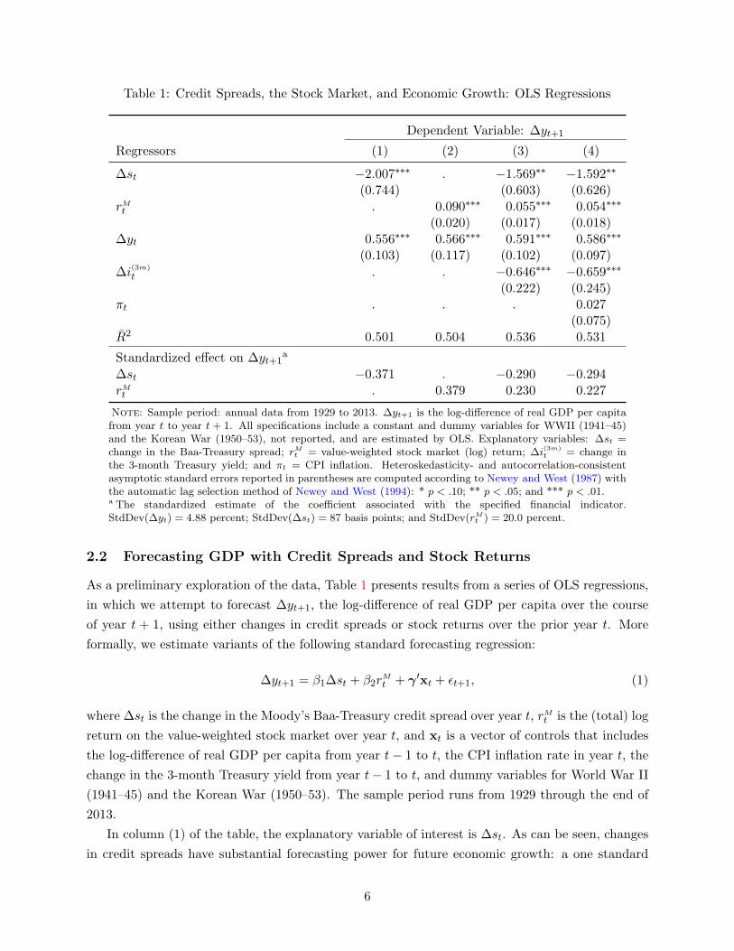
Table 1: Credit Spreads, the Stock Market, and Economic Growth: OLS Regressions
Note: Sample period: annual data from 1929 to 2013. ∆yt+1 is the log-difference of real GDP per capitafrom year t to year t + 1. All specifications include a constant and dummy variables for WWII (1941–45)and the Korean War (1950–53), not reported, and are estimated by OLS. Explanatory variables: ∆st =change in the Baa-Treasury spread; rM
t = value-weighted stock market (log) return; ∆i(3m)
t = change inthe 3-month Treasury yield; and πt = CPI inflation. Heteroskedasticity- and autocorrelation-consistentasymptotic standard errors reported in parentheses are computed according to Newey and West (1987) withthe automatic lag selection method of Newey and West (1994): * p < .10; ** p < .05; and *** p < .01.a The standardized estimate of the coefficient associated with the specified financial indicator.StdDev(∆yt) = 4.88 percent; StdDev(∆st) = 87 basis points; and StdDev(rM
t ) = 20.0 percent.
2.2 Forecasting GDP with Credit Spreads and Stock Returns
As a preliminary exploration of the data, Table 1 presents results from a series of OLS regressions,
in which we attempt to forecast ∆yt+1, the log-difference of real GDP per capita over the course
of year t + 1, using either changes in credit spreads or stock returns over the prior year t. More
formally, we estimate variants of the following standard forecasting regression:
∆yt+1 = β1∆st + β2rM
t + γ ′xt + ǫt+1, (1)
where ∆st is the change in the Moody’s Baa-Treasury credit spread over year t, rMt is the (total) log
return on the value-weighted stock market over year t, and xt is a vector of controls that includes
the log-difference of real GDP per capita from year t− 1 to t, the CPI inflation rate in year t, the
change in the 3-month Treasury yield from year t− 1 to t, and dummy variables for World War II
(1941–45) and the Korean War (1950–53). The sample period runs from 1929 through the end of
2013.
In column (1) of the table, the explanatory variable of interest is ∆st. As can be seen, changes
in credit spreads have substantial forecasting power for future economic growth: a one standard
6
deviation increase in credit spreads—almost 90 basis points—is associated with a step-down in real
GDP growth per capita of 0.37 standard deviations, or about 1.8 percentage points. In column (2),
we repeat the exercise, replacing ∆st with rMt . In this simple exercise, the forecasting power of the
stock market is strikingly similar to that of the corporate bond market: a one standard deviation
increase in the broad stock market—20 percent—predicts an increase in the next year’s real GDP
growth per capita of 0.38 standard deviations.6 In columns (3) and (4), we let ∆st and rMt enter
the regression together and also add two other explanatory variables, the change in the 3-month
Treasury yield (∆i(3m)
t ) and the inflation rate (πt). In both cases, the horse race between credit
spreads and stock returns appears to produce a virtual draw, with each of the two returns retaining
statistically significant and economically similar predictive power for future output growth.
2.3 Financial-Market Sentiment and Economic Activity: Baseline Results
Of course, there is good reason to think that the above predictive relationships may not be causal.
Economic activity may move around for a variety of exogenous nonfinancial reasons, and forward-
looking credit spreads and stock prices may simply anticipate these changes. In this section, we try
to isolate the component of asset price movements that comes from an unwinding of past investor
sentiment, as opposed to changes in expectations of future cashflows.
As described earlier, we do so by means of a two-step regression specification. In the first step,
we use a set of valuation indicators to forecast future changes in credit spreads and stock returns.
We then take the fitted values from the first stage, which we interpret as capturing fluctuations
in financial-market sentiment, and use them in a second regression to predict changes in various
measures of economic activity. Formally, our econometric method consists of the following set of
equations:
∆st = θ′1z1,t−2 + ν1t; (2)
rM
t = θ′2z2,t−1 + ν2t; (3)
∆yt+h = β1∆st + β2rM
t + γ ′xt + ǫt+h; (h ≥ 0), (4)
where ∆st = θ′
1z1,t−2 and rMt = θ
′
2z2,t−1. The first two forecasting regressions project current
changes in credit spreads and stock returns on two- and one-year lagged valuation indicators,
denoted by z1,t−2 and z2,t−1, respectively. The third equation estimates the effect that variation
in these expected returns has on current and future economic activity. To take into account the
generated-regressor nature of the expected returns, the above system of equations is estimated
jointly by nonlinear least squares (NLLS).7
Table 2 presents our baseline results, corresponding to the forecast horizon h = 0. Consider first
6Research documenting the predictive power of stock returns for future economic activity can be traced back toFama (1981) and Fischer and Merton (1984).
7Statistical inference of the parameters of interest is based on a heteroskedascticity- and autocorrelation-consistentasymptotic covariance matrix computed according to Newey and West (1987), utilizing the automatic lag selectionmethod of Newey and West (1994).
7
Table 2: Financial-Market Sentiment and Economic Growth
Note: Sample period: annual data from 1929 to 2013. The main dependent variable is ∆yt, the log-difference of real GDP per capita from year t−1 to year t. Explanatory variables: ∆st = predicted changein the Baa-Treasury spread; rM
t = predicted value-weighted stock market (log) return; and rSPt = predicted
S&P 500 (log) return. Additional explanatory variables (not reported) include dummy variables for WWII(1941–45) and the Korean War (1950–53). In the auxiliary forecasting equations: HYSt = fraction ofdebt that is rated as high yield (Greenwood and Hanson, 2013, the coefficient is multiplied by 100); ESt =equity share in total (debt + equity) new issues (Baker and Wurgler, 2000); [D/P ]t = dividend-price ratiofor the (value-weighted) stock market; and [P/E]t = cyclically adjusted P/E ratio for the S&P 500 (Shiller,2000). All specifications include a constant (not reported) and are estimated jointly with their auxiliaryforecasting equation(s) by NLLS. Heteroskedasticity- and autocorrelation-consistent asymptotic standarderrors reported in parentheses are computed according to Newey and West (1987) with the automatic lagselection method of Newey and West (1994): * p < .10; ** p < .05; and *** p < .01.
column (1) and begin by focusing on the lower panel of the table. Here is the first-step regression, in
which we predict ∆st with two variables: (1) the log of HYSt−2, where HYSt−2 denotes high-yield
bond issuance in year t− 2, expressed as share of total bond issuance in the nonfinancial corporate
sector in that year; and (2) st−2, the level of the Baa-Treasury credit spread at the end of year t−2.
Again, this approach to forecasting ∆st is taken directly from Greenwood and Hanson (2013).8 As
8We also follow GH by defining HYSt−2 based on the fraction of nonfinancial (gross) bond issuance in a givenyear that is rated by Moody’s as below investment grade.
8
can be seen, the log of HYSt−2 enters with a significantly positive coefficient, implying that an
elevated level of the high-yield share in year t− 2 predicts a subsequent widening of credit spreads
in year t. And st−2 enters with a negative coefficient, which implies that when the credit spread is
low in year t − 2, it is expected to mean revert over the course of year t. Notably, the first-stage
regression with these two predictors yield an R2 of 0.095, so our valuation measures are reasonably
powerful in predicting future movements in credit spreads. All of this is closely consistent with the
results reported in Greenwood and Hanson (2013).
Turning to the upper panel of Table 2, column (1) shows that this approach yields an estimate of
the impact of ∆st on ∆yt that is strongly statistically significant and, if anything, larger (in absolute
terms) than that obtained with OLS: the estimated coefficient on ∆st is −5.24, as compared to
an OLS coefficient of −2.01 on ∆st in column (1) of Table 1. We interpret this as saying that the
component of credit-spread changes that is driven by a reversal of prior sentiment has a significant
impact on economic activity. This finding is our central result.
In column (2) of Table 2, we replace ∆st with the fitted stock market return rMt and use
lagged values of the log of the dividend-price ratio (log[D/P ]t−1) and the log of the equity share
(log ESt−1) as predictors for rMt . Note that these predictors for rM
t are based on t− 1 values, rather
than the t − 2 values that we used to predict ∆st. We do this because when we use more distant
lags of stock-market sentiment indicators, our ability to forecast stock returns weakens significantly,
and for our purposes, we are interested in giving the stock market the best possible opportunity to
compete with the corporate bond market, even if this means stacking the deck somewhat in favor
of the former. Nevertheless, even with this edge, the estimate of the effect of the expected return
rMt on output growth is economically small and statistically insignificant.
In column (3), we use an alternative predictor for the stock market return, the log of the lagged
cyclically-adjusted price-earnings ratio (log[P/E]t−1) for the S&P 500 stock price index (Shiller,
2000). For consistency, we also redefine the market return so that it is based on the S&P 500 index,
rather than on the entire value-weighted market index. With this adjustment, the coefficient on
the expected stock market return becomes marginally significant.9 Finally, in columns (4) and (5),
we run horse races by including fitted values of both ∆st and rMt in the second-stage regression
simultaneously and forecasting each of them as before. Now the fitted change in the credit spread
is the clear winner: its coefficient is almost identical to that from column (1), while the coefficients
on the fitted stock market return are close to zero and statistically insignificant, regardless of the
valuation indicators used to predict stock returns.
Thus, unlike the results in Table 1, those in Table 2 point to a sharp distinction between credit
spreads and stock returns. While the two variables fare about equally well in simple OLS forecasting
regressions, only credit spreads enter robustly when we take a two-step regression approach.10 This
9In unreported regressions, we have experimented with other predictors for future stock returns in the first-stageregression, such as the consumption-wealth ratio (Lettau and Ludvigson, 2001). These too lead to insignificantestimates of the coefficient on fitted stock returns in the second stage.
10This divergence cannot be explained based on the first-step forecasting regressions for stock returns being lesspowerful than those for credit spreads. As can be seen by comparing the bottom panel of Table 2, these first-stepregressions have similar R2 values. Thus, the problem is not that stock returns cannot be predicted; rather, it is that
9
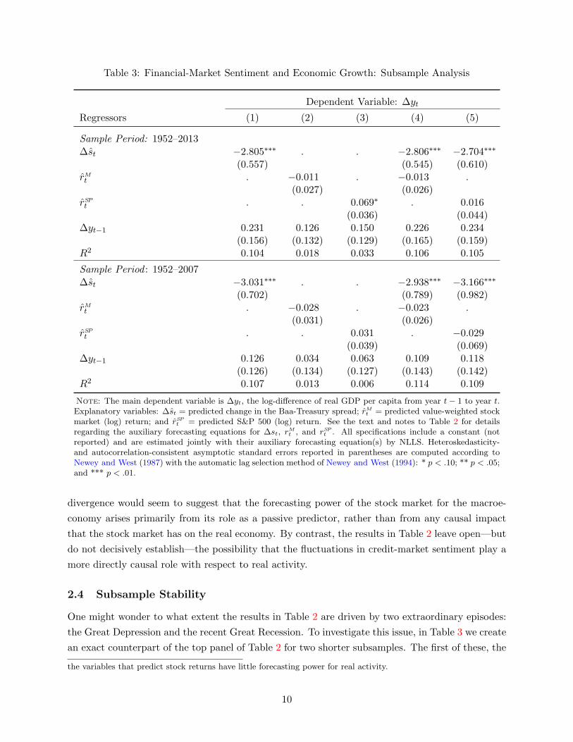
Table 3: Financial-Market Sentiment and Economic Growth: Subsample Analysis
Note: The main dependent variable is ∆yt, the log-difference of real GDP per capita from year t− 1 to year t.Explanatory variables: ∆st = predicted change in the Baa-Treasury spread; rM
t = predicted value-weighted stockmarket (log) return; and rSP
t = predicted S&P 500 (log) return. See the text and notes to Table 2 for detailsregarding the auxiliary forecasting equations for ∆st, rM
t , and rSPt . All specifications include a constant (not
reported) and are estimated jointly with their auxiliary forecasting equation(s) by NLLS. Heteroskedasticity-and autocorrelation-consistent asymptotic standard errors reported in parentheses are computed according toNewey and West (1987) with the automatic lag selection method of Newey and West (1994): * p < .10; ** p < .05;and *** p < .01.
divergence would seem to suggest that the forecasting power of the stock market for the macroe-
conomy arises primarily from its role as a passive predictor, rather than from any causal impact
that the stock market has on the real economy. By contrast, the results in Table 2 leave open—but
do not decisively establish—the possibility that the fluctuations in credit-market sentiment play a
more directly causal role with respect to real activity.
2.4 Subsample Stability
One might wonder to what extent the results in Table 2 are driven by two extraordinary episodes:
the Great Depression and the recent Great Recession. To investigate this issue, in Table 3 we create
an exact counterpart of the top panel of Table 2 for two shorter subsamples. The first of these, the
the variables that predict stock returns have little forecasting power for real activity.
10
Figure 2: Credit-Market Sentiment and Economic Growth
-15
-12
-9
-6
-3
0
3
6
9
12
-1.2 -0.9 -0.6 -0.3 0.0 0.3 0.6
Predicted change in Baa-Treasury spread at t (pps.)
Res
idua
l rea
l GD
P p
er c
apita
gro
wth
at t
(pc
t.)
1931 - 1934
2008 - 2013
1934
Note: Sample period: annual data from 1929 to 2013. The x-axis shows the predicted values of ∆st—the changein the Baa-Treasury spread from year t− 1 to year t—from the auxiliary forecasting regression in column 1 ofTable 2. The y-axis shows the log-difference of real GDP per capita (×100) from t− 1 to t after controlling forlagged dynamics, WWII, and the Korean War (see the text for details).
upper panel of the table, covers a sample period from 1952 to 2013, thereby excluding the Great
Depression and the roughly 15 years that followed. The latter, in the lower panel, covers a sample
period from 1952 to 2007, thereby excluding both the Great Depression and the Great Recession.
In both cases, the results for these two subsamples run closely parallel to those for the full sample
period. The estimated coefficients on ∆st remain strongly significant, albeit noticeably smaller
than their full sample counterparts. Moreover, the coefficients on the two measures of fitted stock
returns remain insignificant across almost all specifications. Overall, it appears that our full sample
findings are not simply the product of a few influential observations, though it is clear that adding
the Great Depression to the sample does contribute to larger (in absolute terms) point estimates.
Figure 2 investigates this issue further, providing a graphical illustration of the results in col-
umn (1) of Table 2. For each year in our full sample period, we plot the residual value of real GDP
growth per capita (obtained from a regression of GDP growth on the other covariates in the model)
against the fitted value ∆st from our auxiliary forecasting regression. The slope of the line in this
picture thus corresponds directly to the estimate of the coefficient on ∆st reported in column (1) of
Table 2. We then highlight the specific data points corresponding to the Great Depression and the
Great Recession. Doing so makes it apparent that these data points are not primarily responsible
11
Figure 3: Time-Varying Credit-Market Sentiment and Economic Growth
Time-varying coefficientFull-sample coefficientStatistically significant at the 1% levelStatistically significant at the 5% levelStatistically significant at the 10% level
Note: The dependent variable is ∆yt, the log-difference of real GDP per capita from year t − 1 to year t.The solid line depicts the time-varying NLLS estimate of the coefficient associated with ∆st, the predictedchange in the Baa-Treasury spread, based on the rolling 40-year window (the dashed line shows the full sampleestimate from column 1 in Table 2). The explanatory variables in the auxiliary forecasting equation for ∆st arelogHYSt−2 and st−2 (see the text and notes to Table 2 for details).
for driving the slope of the regression line.
In Figure 3, we explore subsample stability in an alternative way. Here we estimate the coeffi-
cient on ∆st exactly as in column (1) of Table 2, but on a rolling sample with a 40-year window.
We then plot the time series of these rolling estimates (the convention here is that the data point
labeled “1975” reflects an estimate based on the sample period 1935–1975). As the figure shows,
while this series was quite jumpy as the Great Depression years moved out of the sample window—
reflecting the very large outliers in these years—the estimates have been remarkably stable over the
last 35 or so years, which collectively reflect data from the post-Depression period. And notably,
the more recent Great Recession period does not appear to have had a marked influence on the
coefficient estimates.
Taken together, therefore, the evidence in Table 3, as well as that in Figures 2 and 3, strongly
indicates that our results are not simply the product of the most extreme financial crises of the last
century. Instead, they appear to reflect—at least in substantial part—the influence of less extreme,
but more frequently occurring fluctuations in the pricing of credit risk.
12
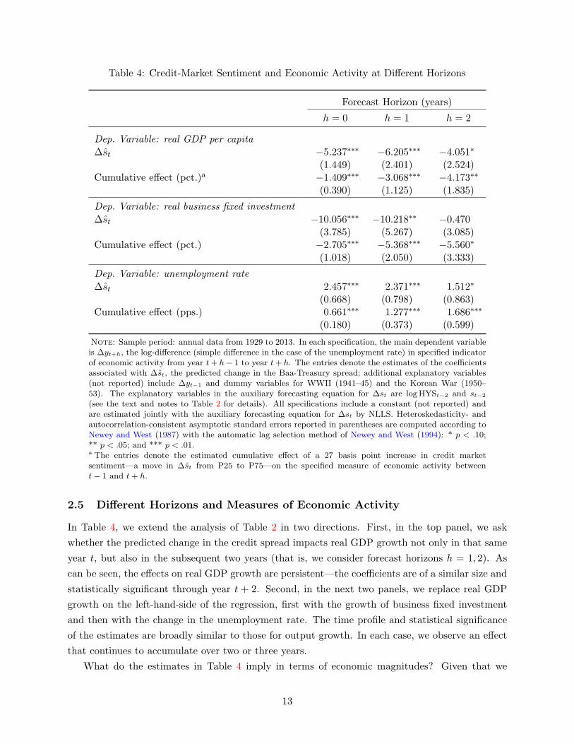
Table 4: Credit-Market Sentiment and Economic Activity at Different Horizons
Note: Sample period: annual data from 1929 to 2013. In each specification, the main dependent variableis ∆yt+h, the log-difference (simple difference in the case of the unemployment rate) in specified indicatorof economic activity from year t+ h− 1 to year t+ h. The entries denote the estimates of the coefficientsassociated with ∆st, the predicted change in the Baa-Treasury spread; additional explanatory variables(not reported) include ∆yt−1 and dummy variables for WWII (1941–45) and the Korean War (1950–53). The explanatory variables in the auxiliary forecasting equation for ∆st are log HYSt−2 and st−2
(see the text and notes to Table 2 for details). All specifications include a constant (not reported) andare estimated jointly with the auxiliary forecasting equation for ∆st by NLLS. Heteroskedasticity- andautocorrelation-consistent asymptotic standard errors reported in parentheses are computed according toNewey and West (1987) with the automatic lag selection method of Newey and West (1994): * p < .10;** p < .05; and *** p < .01.a The entries denote the estimated cumulative effect of a 27 basis point increase in credit marketsentiment—a move in ∆st from P25 to P75—on the specified measure of economic activity betweent− 1 and t+ h.
2.5 Different Horizons and Measures of Economic Activity
In Table 4, we extend the analysis of Table 2 in two directions. First, in the top panel, we ask
whether the predicted change in the credit spread impacts real GDP growth not only in that same
year t, but also in the subsequent two years (that is, we consider forecast horizons h = 1, 2). As
can be seen, the effects on real GDP growth are persistent—the coefficients are of a similar size and
statistically significant through year t + 2. Second, in the next two panels, we replace real GDP
growth on the left-hand-side of the regression, first with the growth of business fixed investment
and then with the change in the unemployment rate. The time profile and statistical significance
of the estimates are broadly similar to those for output growth. In each case, we observe an effect
that continues to accumulate over two or three years.
What do the estimates in Table 4 imply in terms of economic magnitudes? Given that we
13
are interested in understanding the effects of ex ante fluctuations in credit-market sentiment on
real economic outcomes, perhaps the most useful way to think about the magnitudes implied by
the regression coefficients is in terms of a plausibly-sized shock to the fitted value ∆st. Thus for
example, we can ask what the implications are for cumulative output growth over the period from t
to t+2 when ∆st—which is our proxy for credit-market sentiment—moves from the 25th to the 75th
percentile of its distribution, which corresponds to a roughly 30 basis point increase in ∆st. For real
GDP per capita, the answer is that the cumulative growth impact from a sentiment move of this
magnitude is around 4.2 percentage points. And, again, it bears emphasizing that in undertaking
this thought experiment, we are asking how movements in output growth over years t through t+2
respond to changes in the year t−2 value of sentiment. Seen in this light, the economic magnitudes
implied by our estimates would seem to be quite large.
For the other economic variables, we obtain similarly sizable magnitudes. The same 25th-to-
75th-percentile swing in credit-market sentiment as of t − 2 forecasts a cumulative decline in real
business fixed investment of around 5.6 percentage points over the period t to t+2, and a cumulative
increase in the unemployment rate of about 1.7 percentage points.
2.6 The Term Spread as an Additional Indicator of Credit-Market Sentiment
Thus far, we have followed Greenwood and Hanson (2013) closely and have used the two variables
that they highlight—lagged values of the credit spread and the high-yield share—as our only pre-
dictors of changes in credit spreads. We have done so in part to discipline ourselves against the
temptation to mine the data for other variables that may also forecast credit returns.
In Table 5, we relax this discipline a bit. We add an additional variable to our forecasting
regression for ∆st, namely the level of the term spread at the end of year t − 2, defined as the
difference between yields on 10-year and 3-month Treasury securities. Over the full sample period
from 1929 to 2013, it turns out that the term spread has substantial predictive power for future
changes in corporate bond credit spreads. It attracts a significantly negative coefficient, while
the coefficients on the other two measures of credit-market sentiment remain roughly unchanged;
moreover, the R2 of the first-step forecasting regression increases notably, from 0.095 to 0.134.
With this expanded set of variables, the estimate of the impact of ∆st on ∆yt declines slightly in
absolute magnitude, from −5.24 to −4.23. However, given that we are ultimately interested in the
effect of changes in ex ante credit-market sentiment, it is important to recognize that with the added
variable in the first-step regression, we now trace out more variation in sentiment—that is, the fitted
value ∆st now has more variance. Therefore, when we redo the economic significance calculations
of the sort shown in Table 4, we actually get either similar or somewhat larger cumulative impacts.
These results are displayed in Table 6, which is identical in structure to Table 4 but rests on first-
step estimates which use the expanded set of predictors including the term spread. For example,
with this alternative specification, a move in ∆st from the 25th to the 75th percentile of its historical
distribution is now about 50 basis points instead of around 30 basis points and leads to a cumulative
increase in the unemployment rate of 3.2 percentage points over years t to t+2, as compared with
14
Table 5: Credit-Market Sentiment and Economic Growth(Alternative Measures of Credit-Market Sentiment)
Note: The main dependent variable is ∆yt, the log-difference of real GDP per capita from year t − 1 to year t.Explanatory variables: ∆st = predicted change in the Baa-Treasury spread; for the 1929–2013 sample period,additional explanatory variables (not reported) include dummy variables for WWII (1941–45) and the KoreanWar (1950–53). In the auxiliary forecasting equations: HYSt = fraction of debt that is rated as high yield(Greenwood and Hanson, 2013, the coefficient is multiplied by 100); and TSt = term spread. All specificationsinclude a constant (not reported) and are estimated jointly with their auxiliary forecasting equation for ∆st byNLLS. Heteroskedasticity- and autocorrelation-consistent asymptotic standard errors reported in parentheses arecomputed according to Newey and West (1987) with the automatic lag selection method of Newey and West (1994):* p < .10; ** p < .05; and *** p < .01.
an increase of 1.7 percentage points reported in Table 4.
Finally, the last four columns of Table 5 redo the analysis of the first two columns of the table,
but restricting attention to the subsample periods 1952–2013 and 1952–2007. As can be seen, both
the first- and second-step regression results are very robust to the inclusion of the term spread in
these two subsamples. Thus taken together, Tables 5 and 6 indicate that, if anything, adding the
term spread as a first-stage indicator of sentiment strengthens all of our baseline results.
2.7 Controlling for Corporate Leverage
As noted above, our two-step methodology should not be thought of as an IV estimation strategy
because of what is effectively an exclusion-restriction violation: the possibility remains that our
credit-market sentiment variables influence economic activity not via their impact on future changes
in credit supply, but through some other channel. Although we can never directly rule out all
potential stories along these lines, we can investigate some of the more obvious possibilities. For
example, one natural hypothesis is that when the credit market is buoyant and junk bond issuance
is running at high levels, the leverage of operating firms is rising, and it is this increased leverage,
15
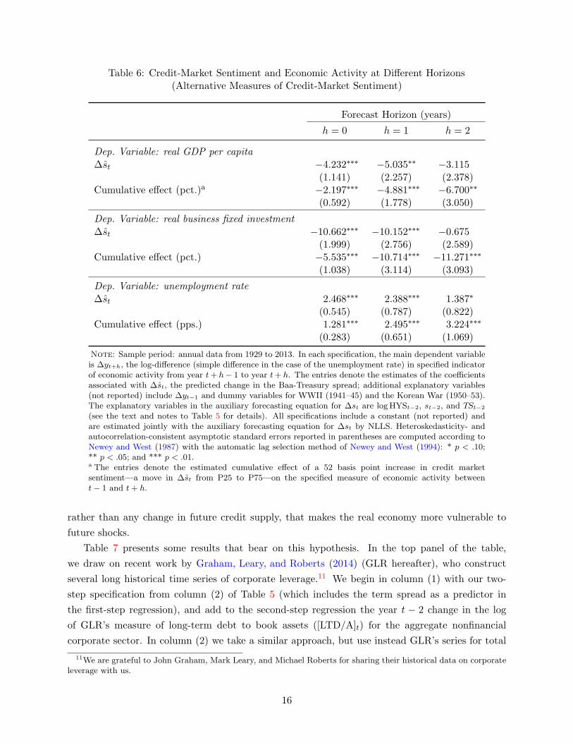
Table 6: Credit-Market Sentiment and Economic Activity at Different Horizons(Alternative Measures of Credit-Market Sentiment)
Note: Sample period: annual data from 1929 to 2013. In each specification, the main dependent variableis ∆yt+h, the log-difference (simple difference in the case of the unemployment rate) in specified indicatorof economic activity from year t+ h− 1 to year t+ h. The entries denote the estimates of the coefficientsassociated with ∆st, the predicted change in the Baa-Treasury spread; additional explanatory variables(not reported) include ∆yt−1 and dummy variables for WWII (1941–45) and the Korean War (1950–53).The explanatory variables in the auxiliary forecasting equation for ∆st are log HYSt−2, st−2, and TSt−2
(see the text and notes to Table 5 for details). All specifications include a constant (not reported) andare estimated jointly with the auxiliary forecasting equation for ∆st by NLLS. Heteroskedasticity- andautocorrelation-consistent asymptotic standard errors reported in parentheses are computed according toNewey and West (1987) with the automatic lag selection method of Newey and West (1994): * p < .10;** p < .05; and *** p < .01.a The entries denote the estimated cumulative effect of a 52 basis point increase in credit marketsentiment—a move in ∆st from P25 to P75—on the specified measure of economic activity betweent− 1 and t+ h.
rather than any change in future credit supply, that makes the real economy more vulnerable to
future shocks.
Table 7 presents some results that bear on this hypothesis. In the top panel of the table,
we draw on recent work by Graham, Leary, and Roberts (2014) (GLR hereafter), who construct
several long historical time series of corporate leverage.11 We begin in column (1) with our two-
step specification from column (2) of Table 5 (which includes the term spread as a predictor in
the first-step regression), and add to the second-step regression the year t − 2 change in the log
of GLR’s measure of long-term debt to book assets ([LTD/A]t) for the aggregate nonfinancial
corporate sector. In column (2) we take a similar approach, but use instead GLR’s series for total
11We are grateful to John Graham, Mark Leary, and Michael Roberts for sharing their historical data on corporateleverage with us.
16
Table 7: Credit-Market Sentiment, Leverage, and Economic Growth
Dependent Variable: ∆yt
Regressors (1) (2) (3)
Aggregate Leverage Measures (1929–2012)
∆st −4.315∗∗∗ −4.320∗∗∗ −4.306∗∗∗
(1.155) (1.108) (1.121)∆ log[LTD/A]t−2 0.006 . .
(0.029)∆ log[TD/A]t−2 . 0.006 .
(0.029)∆ log[TL/A]t−2 . . −0.022
(0.085)R2 0.397 0.396 0.397
Cross-Sectional Percentiles of Leverage (1952–2013)
Note: The main dependent variable is ∆yt, the log-difference of real GDP per capita from year t − 1 toyear t. Explanatory variables: ∆st = predicted change in the Baa-Treasury spread and growth in variousmeasures of corporate leverage: [LTD/A]t = long-term debt to assets; [TD/A]t = total debt to assets; and[TL/A]t = total liabilities to assets. Specifications in the top panel also include ∆yt−1 and dummy variablesfor WWII (1941–45) and the Korean War (1950–53), while those in the bottom panel include ∆yt−1 (notreported). Measures of aggregate leverage are from Graham, Leary, and Roberts (2014), while P50, P75, andP90 denote the (sales-weighted) 50th, 75th, and 90th cross-sectional percentiles, respectively, of the long-termdebt to assets ratio ([LTD/A]t) calculated from firm-level Compustat data. The explanatory variables in theauxiliary forecasting equation for ∆st are logHYSt−2, st−2, and TSt−2, where HYSt denotes the fraction ofdebt that is rated as high yield (Greenwood and Hanson, 2013) and TSt is the term spread. All specificationsinclude a constant (not reported) and are estimated jointly with the auxiliary forecasting equation for ∆st byNLLS. Heteroskedasticity- and autocorrelation-consistent asymptotic standard errors reported in parenthesesare computed according to Newey and West (1987) with the automatic lag selection method of Newey and West(1994): * p < .10; ** p < .05; and *** p < .01.
debt to book assets ([TD/A]t), while in column (3), we use their broader measure of total liabilities
to assets ([TL/A]t). In all three cases, we obtain a similar result: the coefficients on the change-
in-leverage proxies are completely insignificant, and our estimates of the coefficient on ∆st are
virtually unchanged from their value of −4.23 reported in column (2) of Table 5. In further results
(not reported), we find that nothing is altered if we instead enter the GLR leverage variables in
(log) levels, rather than in changes, or use multiple lags of leverage and let the regression pick the
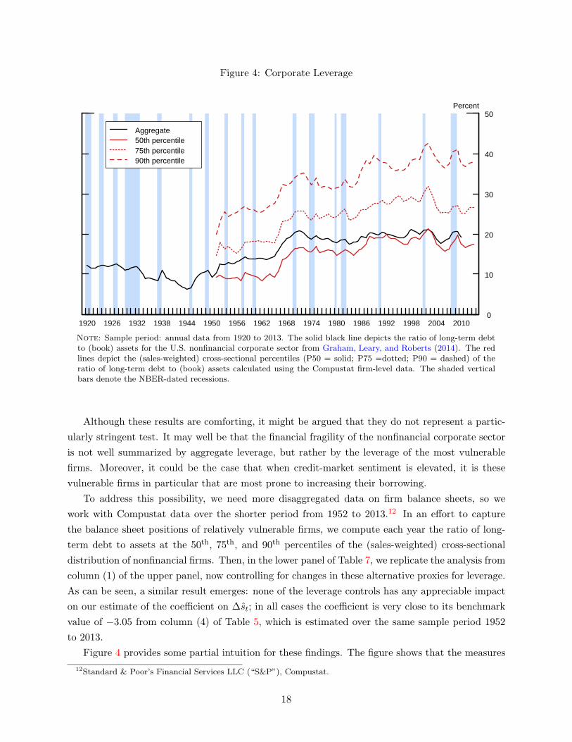
Note: Sample period: annual data from 1920 to 2013. The solid black line depicts the ratio of long-term debtto (book) assets for the U.S. nonfinancial corporate sector from Graham, Leary, and Roberts (2014). The redlines depict the (sales-weighted) cross-sectional percentiles (P50 = solid; P75 =dotted; P90 = dashed) of theratio of long-term debt to (book) assets calculated using the Compustat firm-level data. The shaded verticalbars denote the NBER-dated recessions.
Although these results are comforting, it might be argued that they do not represent a partic-
ularly stringent test. It may well be that the financial fragility of the nonfinancial corporate sector
is not well summarized by aggregate leverage, but rather by the leverage of the most vulnerable
firms. Moreover, it could be the case that when credit-market sentiment is elevated, it is these
vulnerable firms in particular that are most prone to increasing their borrowing.
To address this possibility, we need more disaggregated data on firm balance sheets, so we
work with Compustat data over the shorter period from 1952 to 2013.12 In an effort to capture
the balance sheet positions of relatively vulnerable firms, we compute each year the ratio of long-
term debt to assets at the 50th, 75th, and 90th percentiles of the (sales-weighted) cross-sectional
distribution of nonfinancial firms. Then, in the lower panel of Table 7, we replicate the analysis from
column (1) of the upper panel, now controlling for changes in these alternative proxies for leverage.
As can be seen, a similar result emerges: none of the leverage controls has any appreciable impact
on our estimate of the coefficient on ∆st; in all cases the coefficient is very close to its benchmark
value of −3.05 from column (4) of Table 5, which is estimated over the same sample period 1952
to 2013.
Figure 4 provides some partial intuition for these findings. The figure shows that the measures
Note: Sample period: annual data from 1929 to 2013. The main dependent variable is ∆yt, thelog-difference of real GDP per capita from year t−1 to year t. Explanatory variables: ∆st = predictedchange in the Baa-Treasury spread and 5-year (annualized) growth in various measures of commercialbank balance sheets: BCt = (inflation-adjusted) bank credit (loans + securities); and TLt = (inflation-adjusted) bank loans. Additional explanatory variables (not reported) include ∆yt−1 and dummyvariables for WWII (1941–45) and the Korean War (1950–53). The explanatory variables in theauxiliary forecasting equation for ∆st (columns 3–4) are logHYSt−2, st−2, and TSt−2, where HYSt
denotes the fraction of debt that is rated as high yield (Greenwood and Hanson, 2013) and TSt isthe term spread. All specifications include a constant (not reported) and those in columns 1–2 areestimated by OLS, while those in columns 3–4 are estimated jointly with the auxiliary forecastingequation for ∆st by NLLS. Heteroskedasticity- and autocorrelation-consistent asymptotic standarderrors reported in parentheses are computed according to Newey and West (1987) with the automaticlag selection method of Newey and West (1994): * p < .10; ** p < .05; and *** p < .01.
of corporate leverage that we examine are generally much smoother than the credit spread series.
The GLR series for aggregate leverage has some low frequency time trends but little discernible
business cycle variation. And while the more skewed 75th and 90th percentile leverage series do
appear to have some co-movement with the business cycle, they have much less in the way of high-
frequency variation than do credit spreads. For example, there is a small run-up in the leverage of
firms at the 90th percentile of the distribution in the few years leading up to the recent financial
crisis, but this run-up looks small in comparison to the overall time trend in the same variable.
2.8 Controlling for Bank Credit Growth
In recent work, Schularick and Taylor (2012) and Jorda, Schularick, and Taylor (2013) document
that lagged bank credit growth forecasts future output growth with a negative sign. They interpret
this pattern as evidence that “credit booms gone bust” can have adverse macroeconomic conse-
quences, a hypothesis clearly similar in spirit to ours, albeit more focused on credit extended via
the banking system than via the bond market. Thus, it is of interest to see if there is independent
information in their key predictive variables and ours.
In columns (1) and (2) of Table 8, we run a couple of regressions that echo those of
Schularick and Taylor (2012) and Jorda, Schularick, and Taylor (2013), using our sample and em-
19
pirical framework. In column (1), we run an OLS regression of ∆yt—the log-difference in real GDP
per capita from year t − 1 to year t—on its once-lagged value, and on the log-difference in bank
credit over the 5-year period ending in year t−1 (∆5 log BCt−1). Here bank credit is defined as the
sum of bank loans plus securities holdings. In column (2), we do the same thing, but use instead
the log-difference in just bank loans (∆5 log BLt−1), rather than total bank credit. In both cases,
we obtain statistically significant negative coefficients, confirming that there does indeed appear to
be a dark side to bank credit booms.
In columns (3) and (4), we run horse races that include these bank credit growth variables
alongside the predicted change in the credit spread ∆st. As can be seen, credit-market sentiment
holds up well in competition with the growth in bank balance sheet variables. When pitted against
bank loan growth in column (4), the coefficient on ∆st is actually a bit larger in absolute terms than
its baseline value of −4.23 reported in column (2) of Table 5, while that on bank loan growth is of
the wrong sign and completely insignificant. In column (3), bank credit growth fares a bit better,
retaining marginal statistical significance, but the coefficient on ∆st remains strongly statistically
significant and is only modestly reduced.
While these results are striking, we caution against over-interpreting them. We would not
want to argue that the story that we have in mind is a fundamentally different one than that of
Schularick and Taylor (2012) and Jorda, Schularick, and Taylor (2013), and that we have somehow
managed to separate them in the data. The two stories clearly overlap. For example, it is hard to
imagine that bank loan supply could expand rapidly without putting downward pressure on spreads
in the corporate bond market, as there must be some degree of arbitrage across the two markets.
So perhaps we have just found an alternative measurement technique that does a more robust job
of capturing variation in credit-market sentiment, particularly outside of the most extreme episodes
in our sample period.
At the same time, while the two stories have much in common, they do differ in their emphasis,
and these differences have potentially interesting policy implications. Implicit in the approach
of Schularick and Taylor (2012) and Jorda, Schularick, and Taylor (2013) is the premise that the
banking system is at the center of credit intermediation, and that it is damage to banks that
leads to adverse economic outcomes. This logic implies that a policy focus on safeguarding the
banking system—via higher capital requirements, for example—might be all that is needed to
improve macroeconomic stability. By contrast, our results suggest that disturbances in credit
supply that originate outside of the banking sector—in particular, in the corporate bond market—
can also have significant consequences for economic activity. If this is the case, then a policy
focus that is entirely bank-regulation-centric may be incomplete, a point also made recently by
Feroli, Kashyap, Schoenholtz, and Shin (2014).
20
3 Exploring the Mechanism
In the previous section, we demonstrated that heightened levels of credit-market sentiment are
bad news for future economic activity. As we have outlined, our working hypothesis is that when
sentiment is running high, it is more likely to reverse itself over the next couple of years, and the
associated widening of credit spreads amounts to a reduction in the supply of credit, which in turn
impinges on the real economy. In this section we attempt to further flesh out this credit-supply
hypothesis. We begin with a simple model that illustrates how data on firms’ financing choices
can help untangle credit demand and credit supply effects. We then undertake a series of tests
motivated by the model. In particular, we show that our proxy for credit-market sentiment not
only predicts changes in real activity, but also forecasts changes in the aggregate debt-equity mix
for nonfinancial firms. We also show that, consistent with the model, credit-market sentiment has
more predictive power for both the financing and investment decisions of firms with lower credit
ratings.
3.1 A Simple Model of Credit-Market Sentiment
The model that follows is adapted from Stein (1996), and it is also similar to that in Ma (2014).
Consider a firm that can invest an amount I, which yields a net present value of θf(I), where f(I)
is a concave function, and θ is a measure of the profitability of investment opportunities. The firm
can finance the investment with either newly-raised debt D or equity E, subject to the budget
constraint that I = D + E. To capture the idea that there can be credit-market sentiment, we
allow for the possibility that the credit spread on the debt deviates from its fundamental value by
an amount δ; our sign convention here is that a positive value of δ represents debt that is expensive
relative to a Modigliani-Miller benchmark of frictionless financial markets and vice versa. For
simplicity, we assume that equity is always fairly priced.
The firm also faces a cost of deviating from its optimal debt-to-capital ratio, which is denoted by
d∗. This cost is assumed to be proportional to the scale of the firm and quadratic in the difference
between d∗ and the actual debt-to-capital ratio d ≡ D/I. Thus overall, the firm’s problem is to
choose the level of investment I and its capital structure d to maximize the following objective
function:
θf(I)− δD − Iγ
2
(
d− d∗)2. (5)
There are three terms in the objective function. The first term, θf(I), is the net present value of
investment. The second term, δD, is the relative cost associated with issuing debt as opposed to
equity; this cost can be either positive or negative, depending on the sign of δ. And the third term,
I γ2
(
d− d∗)2, is the cost associated with deviating from the optimal capital structure of d∗.
We can rewrite the firm’s objective function as:
θf(I)− δdI − Iγ
2
(
d− d∗)2. (6)
21
This yields the following first-order conditions with respect to I and d:
θf ′(I) = δd+γ
2
(
d− d∗)2; (7)
d = d∗ −δ
γ. (8)
Substituting equation (8) into equation (7) gives
θf ′(I) = δd∗ −δ2
2γ. (9)
Equations (8) and (9) express the firm’s choice of capital structure d and investment I as
functions of the exogenous parameters. In so doing, they make clear the identification problem
that arises in interpreting our results from the previous section. Suppose we know that elevated
credit-market sentiment at time t−2 forecasts a decline in investment at time t. This could be either:
(1) because the sentiment proxy is able to forecast a reduction in the appeal of future investment θ,
as would be implied by a story where high levels of sentiment are associated with over-investment
or mis-investment; or (2) because the sentiment proxy is able to forecast an increase in the future
cost of borrowing δ. Based on observation of just investment I, one can see from equation (9)
that these two hypotheses cannot be separated. However, equation (8) tells us that looking at the
firm’s financing mix can help in distinguishing between these two stories because the financing mix
is unaffected by θ. Thus if both investment and the debt-to-capital ratio fall, this can only be
explained by an increase in δ—that is, by an inward shift in the supply of credit. This observation
motivates our first set of tests, which focus on relative movements in the aggregate net debt and
net equity issuance of U.S. nonfinancial firms.
The model also suggests a set of cross-sectional tests. These come from noting that if our credit-
sentiment proxy is able to forecast market-wide changes in the effective cost of credit, these changes
should be more pronounced for lower credit-quality firms because such firms have, in effect, a higher
loading on the aggregate market factor. In other words, the ratio of price-to-fundamentals falls by
more for a Caa-rated issuer than for an Aa-rated issuer when market-wide sentiment deteriorates.
Thus if firm i has a lower credit rating than firm j and we are predicting an increase in the market-
wide spread δ, then we should also be predicting that δi will go up by more than δj . This implies
that when credit-market sentiment is elevated at time t− 2, we should expect that at time t firms
with lower credit ratings will manifest both a greater decline in debt issuance relative to investment
(from equation 8) and a larger drop in the level of investment (from equation 9).
We test these predictions below. Before proceeding, however, we note a caveat on the in-
terpretation: these tests can at best provide evidence that is qualitatively consistent with our
credit-supply hypothesis. They cannot be used to make the quantitative case that credit-supply
effects are predominantly responsible for the large macroeconomic effects documented in Section 2.
As one example, while we find that our credit-sentiment proxy forecasts a significant decline in the
capital expenditures of junk-rated firms relative to those of investment-grade firms, we would not
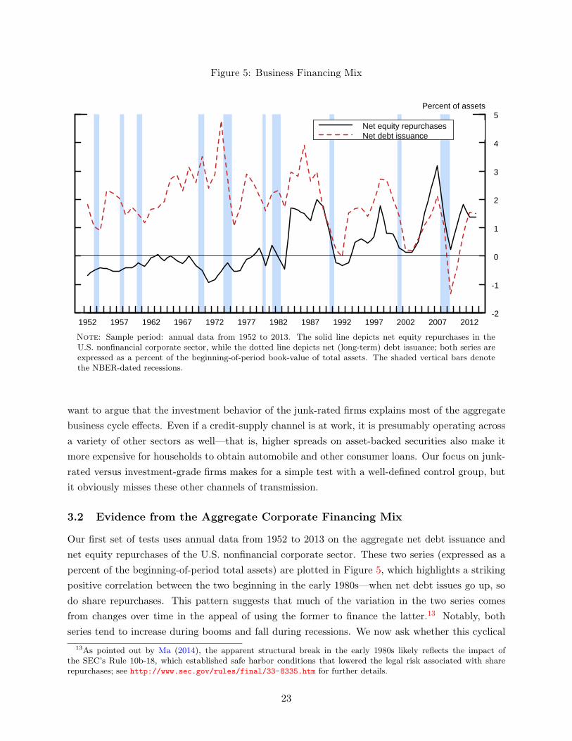
Note: Sample period: annual data from 1952 to 2013. The solid line depicts net equity repurchases in theU.S. nonfinancial corporate sector, while the dotted line depicts net (long-term) debt issuance; both series areexpressed as a percent of the beginning-of-period book-value of total assets. The shaded vertical bars denotethe NBER-dated recessions.
want to argue that the investment behavior of the junk-rated firms explains most of the aggregate
business cycle effects. Even if a credit-supply channel is at work, it is presumably operating across
a variety of other sectors as well—that is, higher spreads on asset-backed securities also make it
more expensive for households to obtain automobile and other consumer loans. Our focus on junk-
rated versus investment-grade firms makes for a simple test with a well-defined control group, but
it obviously misses these other channels of transmission.
3.2 Evidence from the Aggregate Corporate Financing Mix
Our first set of tests uses annual data from 1952 to 2013 on the aggregate net debt issuance and
net equity repurchases of the U.S. nonfinancial corporate sector. These two series (expressed as a
percent of the beginning-of-period total assets) are plotted in Figure 5, which highlights a striking
positive correlation between the two beginning in the early 1980s—when net debt issues go up, so
do share repurchases. This pattern suggests that much of the variation in the two series comes
from changes over time in the appeal of using the former to finance the latter.13 Notably, both
series tend to increase during booms and fall during recessions. We now ask whether this cyclical
13As pointed out by Ma (2014), the apparent structural break in the early 1980s likely reflects the impact ofthe SEC’s Rule 10b-18, which established safe harbor conditions that lowered the legal risk associated with sharerepurchases; see http://www.sec.gov/rules/final/33-8335.htm for further details.
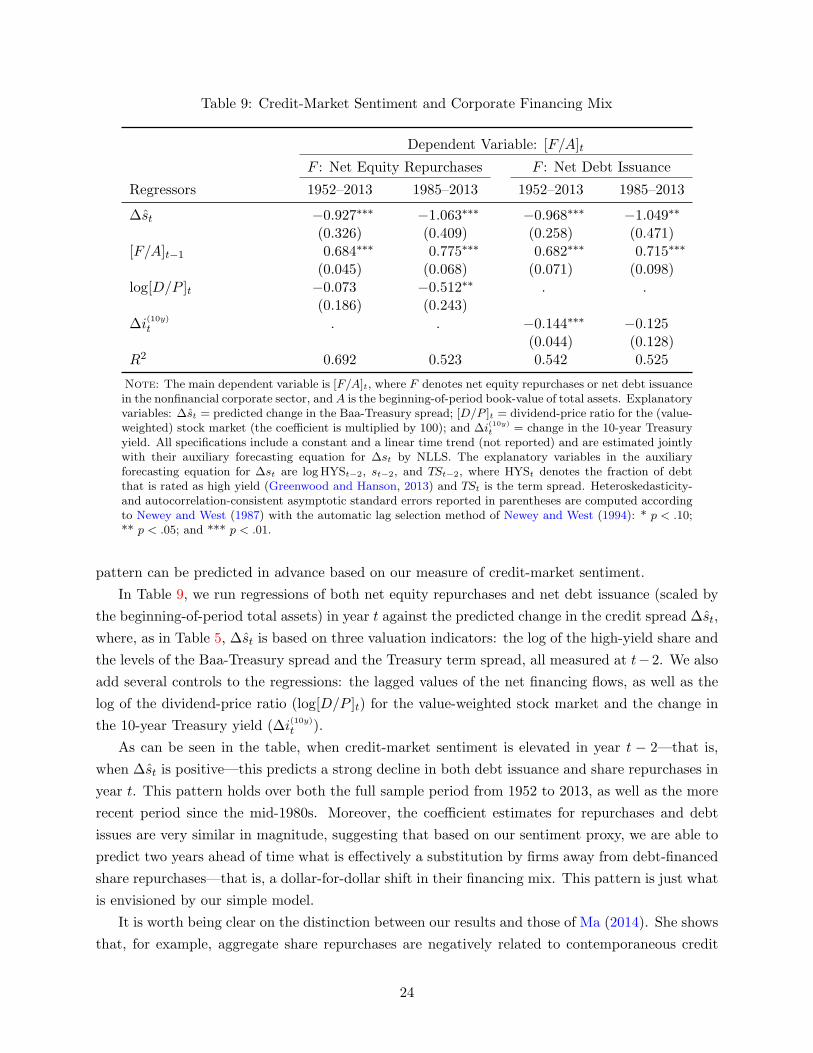
Note: The main dependent variable is [F/A]t, where F denotes net equity repurchases or net debt issuancein the nonfinancial corporate sector, and A is the beginning-of-period book-value of total assets. Explanatoryvariables: ∆st = predicted change in the Baa-Treasury spread; [D/P ]t = dividend-price ratio for the (value-weighted) stock market (the coefficient is multiplied by 100); and ∆i(10y)
t = change in the 10-year Treasuryyield. All specifications include a constant and a linear time trend (not reported) and are estimated jointlywith their auxiliary forecasting equation for ∆st by NLLS. The explanatory variables in the auxiliaryforecasting equation for ∆st are log HYSt−2, st−2, and TSt−2, where HYSt denotes the fraction of debtthat is rated as high yield (Greenwood and Hanson, 2013) and TSt is the term spread. Heteroskedasticity-and autocorrelation-consistent asymptotic standard errors reported in parentheses are computed accordingto Newey and West (1987) with the automatic lag selection method of Newey and West (1994): * p < .10;** p < .05; and *** p < .01.
pattern can be predicted in advance based on our measure of credit-market sentiment.
In Table 9, we run regressions of both net equity repurchases and net debt issuance (scaled by
the beginning-of-period total assets) in year t against the predicted change in the credit spread ∆st,
where, as in Table 5, ∆st is based on three valuation indicators: the log of the high-yield share and
the levels of the Baa-Treasury spread and the Treasury term spread, all measured at t−2. We also
add several controls to the regressions: the lagged values of the net financing flows, as well as the
log of the dividend-price ratio (log[D/P ]t) for the value-weighted stock market and the change in
the 10-year Treasury yield (∆i(10y)t ).
As can be seen in the table, when credit-market sentiment is elevated in year t − 2—that is,
when ∆st is positive—this predicts a strong decline in both debt issuance and share repurchases in
year t. This pattern holds over both the full sample period from 1952 to 2013, as well as the more
recent period since the mid-1980s. Moreover, the coefficient estimates for repurchases and debt
issues are very similar in magnitude, suggesting that based on our sentiment proxy, we are able to
predict two years ahead of time what is effectively a substitution by firms away from debt-financed
share repurchases—that is, a dollar-for-dollar shift in their financing mix. This pattern is just what
is envisioned by our simple model.
It is worth being clear on the distinction between our results and those of Ma (2014). She shows
that, for example, aggregate share repurchases are negatively related to contemporaneous credit
24
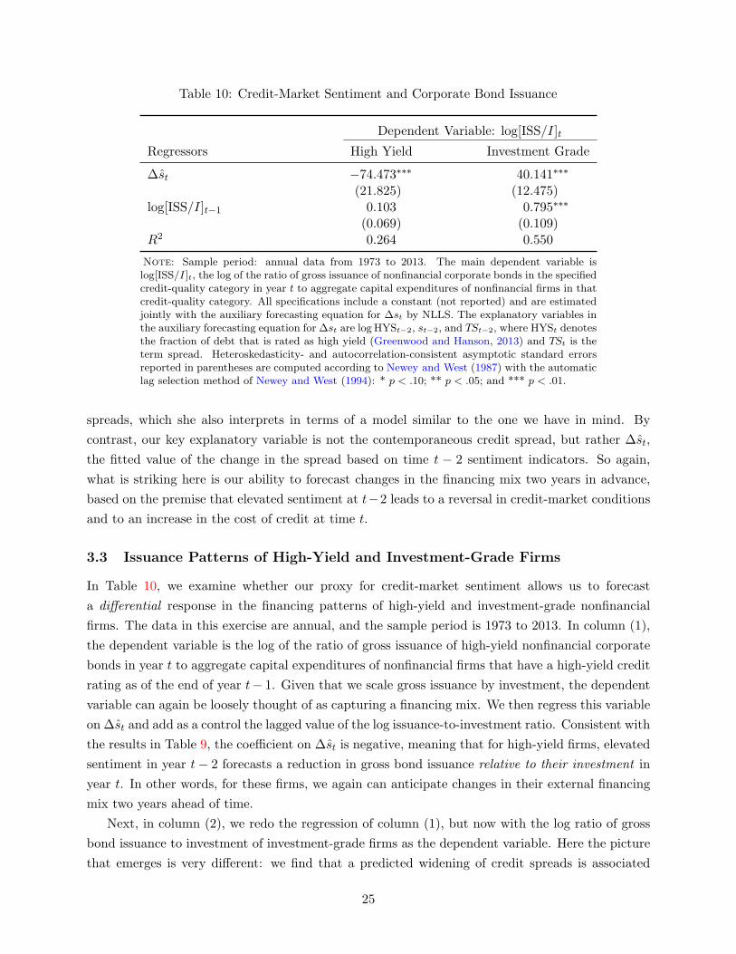
Table 10: Credit-Market Sentiment and Corporate Bond Issuance
Dependent Variable: log[ISS/I]t
Regressors High Yield Investment Grade
∆st −74.473∗∗∗ 40.141∗∗∗
(21.825) (12.475)log[ISS/I]t−1 0.103 0.795∗∗∗
(0.069) (0.109)R2 0.264 0.550
Note: Sample period: annual data from 1973 to 2013. The main dependent variable islog[ISS/I]t, the log of the ratio of gross issuance of nonfinancial corporate bonds in the specifiedcredit-quality category in year t to aggregate capital expenditures of nonfinancial firms in thatcredit-quality category. All specifications include a constant (not reported) and are estimatedjointly with the auxiliary forecasting equation for ∆st by NLLS. The explanatory variables inthe auxiliary forecasting equation for ∆st are log HYSt−2, st−2, and TSt−2, where HYSt denotesthe fraction of debt that is rated as high yield (Greenwood and Hanson, 2013) and TSt is theterm spread. Heteroskedasticity- and autocorrelation-consistent asymptotic standard errorsreported in parentheses are computed according to Newey and West (1987) with the automaticlag selection method of Newey and West (1994): * p < .10; ** p < .05; and *** p < .01.
spreads, which she also interprets in terms of a model similar to the one we have in mind. By
contrast, our key explanatory variable is not the contemporaneous credit spread, but rather ∆st,
the fitted value of the change in the spread based on time t − 2 sentiment indicators. So again,
what is striking here is our ability to forecast changes in the financing mix two years in advance,
based on the premise that elevated sentiment at t−2 leads to a reversal in credit-market conditions
and to an increase in the cost of credit at time t.
3.3 Issuance Patterns of High-Yield and Investment-Grade Firms
In Table 10, we examine whether our proxy for credit-market sentiment allows us to forecast
a differential response in the financing patterns of high-yield and investment-grade nonfinancial
firms. The data in this exercise are annual, and the sample period is 1973 to 2013. In column (1),
the dependent variable is the log of the ratio of gross issuance of high-yield nonfinancial corporate
bonds in year t to aggregate capital expenditures of nonfinancial firms that have a high-yield credit
rating as of the end of year t− 1. Given that we scale gross issuance by investment, the dependent
variable can again be loosely thought of as capturing a financing mix. We then regress this variable
on ∆st and add as a control the lagged value of the log issuance-to-investment ratio. Consistent with
the results in Table 9, the coefficient on ∆st is negative, meaning that for high-yield firms, elevated
sentiment in year t− 2 forecasts a reduction in gross bond issuance relative to their investment in
year t. In other words, for these firms, we again can anticipate changes in their external financing
mix two years ahead of time.
Next, in column (2), we redo the regression of column (1), but now with the log ratio of gross
bond issuance to investment of investment-grade firms as the dependent variable. Here the picture
that emerges is very different: we find that a predicted widening of credit spreads is associated
25
with a significant increase in gross bond issuance by investment-grade firms relative to their capital
expenditures—that is, the result for investment-grade firms goes the “wrong way.” This result
for gross (as opposed to net) issuance may reflect the fact that high-quality corporate borrowers
frequently take advantage of falling long-term interest rates—which are associated with economic
downturns—to restructure their debt by issuing long-term bonds, the proceeds of which are used to
pay down shorter-term, variable-rate obligations such as bank loans. In any event, the pronounced
difference in issuance patterns between high-yield and investment-grade firms is consistent with our
model, under the assumption that a change in market-wide sentiment has a stronger effect on the
δ of a high-yield firm than on the δ of an investment-grade firm.
3.4 Investment Behavior of Firms By Rating Category
Finally, we turn to a comparison of the investment behavior of firms in different credit-rating
categories. To do so, we use firm-level Compustat data from 1973 to 2013 to estimate the following
That is, we regress the change in the log of real capital expenditures for firm j in year t on:
(1) the predicted value of the change in credit spread in year t (∆st), our measure of credit-market
sentiment, again based on year t− 2 valuation indicators; (2) the change in its own log of real sales
in year t (∆ log Yjt); (3) its stock return in year t (rjt); and (4) the change in the log of industrial
production for the firm’s 3-digit NAICS industry in year t (∆ log IPI
t).
To implement our test, we allow all of the coefficients in regression (10) to differ across four
credit-quality buckets (RTGj,t−1): unrated, high yield, low investment grade, and high investment
grade.14 Thus with this specification, we are asking whether elevated credit-market sentiment at
time t − 2 forecasts a more negative outcome for the time-t investment of firms with low credit
ratings than for the time-t investment of firms with high credit ratings. This is after allowing
firms in the four credit-quality buckets to also have a differential response of investment growth
to their own sales growth and stock returns, as well as to fluctuations in industry-level industrial
production. The specification also includes firm fixed effects (ηj), which capture any time-invariant
unobservable firm characteristics, such as, for example, systematic difference in productivity growth
across firms.
The motivation for this extensive set of controls that vary across credit-quality buckets can
be seen in Figure 6, which plots the growth rate of aggregate capital expenditures of those nonfi-
nancial Compustat firms that are rated either as investment grade, speculative grade, or have no
credit rating. As can be seen in the figure, the investment of the unrated and junk-rated firms is
14The Moody’s senior (unsecured) credit ratings—which are as of the end of year t− 1—associated with the fourcategories (RTGj,t−1) are: Unrated = no credit rating; high yield = Ba1, Ba2, Ba3, B1, B2, B3, Caa1, Caa2, Caa3,Ca; low investment grade = A1, A2, A3, Baa1, Baa2, Baa3; and high investment grade = Aaa, Aa1, Aa2, Aa3.
26
Figure 6: Growth of Capital Expenditures by Type of Firm
Note: Sample period: annual data from 1973 to 2013. The solid line depicts line depicts the growth rate ofaggregate capital expenditures of nonfinancial Compustat firms that have, according to Moody’s, an investment-grade credit rating at the beginning of each year; the dotted line depicts the growth rate of aggregate capitalexpenditures of nonfinancial Compustat firms that have a speculative-grade credit rating at the beginning of eachyear; and the dashed line depicts the growth rate of aggregate capital expenditures of nonfinancial Compustatfirms that have no credit rating at the beginning of each year. All series are in $2009. The shaded vertical barsdenote the NBER-dated recessions.
considerably more procyclical than the investment of the investment-grade firms. So we want to be
sure that when we attempt to measure the differential impact of credit-market sentiment on firms
in different credit-rating categories, we control as carefully as possible for the general tendency of
lower credit-quality firms to have more procyclical investment behavior.
The results of this exercise are shown in the upper panel of Table 11. As can be seen, the coeffi-
cients on ∆st are economically large and statistically significant across the lower three credit-quality
buckets. For example, in the high-yield bucket, the coefficient estimate implies that, conditional
on all the other controls in the regression, a 100 basis point increase in time t − 2 credit-market
sentiment (that is, a 100 basis point increase in the predicted change in credit spreads) is associ-
ated with a decline in the growth of capital expenditures for a typical junk-rated firm of almost
7 percentage points from year t − 1 to year t. By contrast, the coefficient on ∆st is economically
small and statistically insignificant for firms in the high investment-grade bucket. Moreover, the
difference between the coefficient for this highest credit-quality bucket and the other three is in
each case strongly significant.
This evidence is broadly consistent with our basic cross-sectional hypothesis, which postulates
that firms with lower credit ratings have both issuance and investment behavior that is more
27
Table 11: Credit-Market Sentiment and Investment by Type of Firm
(3.245) (4.405) (2.354) (2.591)Pr > W <.001 0.014 0.015 .
Obs. per category 52,901 4,804 5,179 1,021
Note: Sample period: annual data from 1973 to 2013. Panel dimensions: No. of firms = 5,553; Tj = 11.5(years); and Total obs. = 63,905. The dependent variable is ∆ log Ijt, the log-difference of real capitalexpenditures of firm j from year t − 1 to year t. Explanatory variables: ∆st = predicted change in theBaa-Treasury spread; ∆ log Yjt = log-difference of real sales of firm j; rjt = total (log) return of firm j; and∆ log IP I
t = log-difference of 3-digit NAICS industrial production. All explanatory variables are interactedwith RTGj,t−1, an indicator of the firm’s credit quality at the end of year t − 1. Unrated = no creditrating; HY (high yield) = Ba1, Ba2, Ba3, B1, B2, B3, Caa1, Caa2, Caa3, Ca; Low IG (lower investmentgrade) = A1, A2, A3, Baa1, Baa2, Baa3; and High IG (high investment grade) = Aaa, Aa1, Aa2, Aa3. Theexplanatory variables in the auxiliary forecasting equation for ∆st are logHYSt−2, st−2 and TSt−2, whereHYSt denotes the fraction of debt that is rated as high yield (Greenwood and Hanson, 2013) and TSt is theterm spread. All specifications includes firm fixed effects and are estimated by OLS. Heteroskedasticity-and autocorrelation-consistent asymptotic standard errors reported in parentheses are computed accordingto Driscoll and Kraay (1998): * p < .10; ** p < .05; and *** p < .01.a p-value of the test that the coefficient on ∆st in the specified credit quality category is equal to that inthe “High IG” category.
sensitive to changes in aggregate credit-market sentiment. However, an important caveat is that
the differential investment results in Table 11 depend on isolating a relatively small group of the
most highly rated firms; the number of firms in this bucket in a typical year averages around 80.
Outside of this small group, we do not find statistically significant differences in the sensitivity of
investment to credit-market sentiment as we move across the three lower credit-quality buckets,
even though the pattern of the point estimates is monotonic in the expected direction.
The fact that we do not find more pronounced differences across the lower credit-quality buckets
may partly reflect an “over-controlling” problem. For example, to the extent that low credit-quality
firms are more badly hurt by an increase in the cost of credit, this is likely to show up to some
degree in both their sales and their stock returns. Given that these controls are—unlike our credit-
28
market sentiment measures—not lagged by two years, they could be picking up some of the effect.
To illustrate this point, we re-estimate regression (10) without any of the controls; these results
are shown in the bottom panel of Table 11. As can be seen, the spread in the coefficients on ∆st
across the credit-quality buckets becomes notably more pronounced than in the prior case with the
full set of controls.
4 Possible Implications for Monetary Policy
Although time-varying credit-market sentiment—or equivalently, a time-varying credit-risk
premium—plays a central role in our narrative, we have been silent on its source of variation,
in effect treating it as exogenous. But what drives this variation in sentiment? One can imagine
a number of potential factors. Mistaken beliefs on the part of investors are one possibility. For
example, after a few years of economic expansion with relatively few defaults, overly-extrapolative
investors might begin to pay too little attention to default risk, leading to compressed credit spreads
(Gennaioli, Shleifer, and Vishny, 2012). However, Stein (2013) argues that while mistaken beliefs
may be important, they are unlikely to be the whole story behind time-varying expected returns
in credit markets, especially given the centrality of financial intermediaries in these markets. Var-
ious contracting frictions and agency problems at the intermediary level are also likely to be an
important part of the mechanism.
One strand of recent literature highlights the importance of intermediaries’ balance sheets. For
example, Adrian, Etula, and Muir (2014) argue that in a world of segmented markets and financ-
ing frictions, the wealth of broker-dealers is effectively the stochastic discount factor that prices
risky assets in the economy—so that when broker-dealer balance sheets are strong, and the marginal
value of their wealth is low, expected returns on risky assets are low as well. He and Krishnamurthy
(2013) develop a dynamic asset pricing model with an intermediary sector that has similar impli-
cations. They also stress that their model is particularly likely to apply to the pricing of various
types of credit risk, as opposed to pinning down the equity market premium.15 Another comple-
mentary line of work focuses on an agency problem between intermediaries and their shareholders
and argues that this agency problem is intensified when the general level of interest rates is low
because it makes intermediaries more likely to “reach for yield”—that is, to accept lower premiums
for bearing duration and credit risk—at such times.16
Although we have not provided any evidence to help parse these different effects, we believe
that our results may have particularly interesting policy implications if one accepts the key premise
of the reach-for-yield literature, namely that accommodative monetary policy is one of the factors
that can lead to a compression of credit-risk premiums. To see this point, suppose that the central
15See also Brunnermeier and Pedersen (2009), Danielsson, Shin, and Zigrand (2011), and Adrian and Boyarchenko(2013) for related work.
16See, for example, Rajan (2006); Borio and Zhu (2008); Jimenez, Ongena, Peydro, and Saurina (2014);Hanson and Stein (2015); and Gertler and Karadi (2015).
29
bank has the following simple objective function:
minEt
∞∑
j=t
βj−t(
Uj − U∗)2
,
where Uj is the unemployment rate at time j, U∗ is the policymaker’s target level for the unem-
ployment rate, and β is a discount factor. Thus, the central bank seeks to minimize the expected
discounted sum of squared deviations of the unemployment rate from its target. Suppose further
that the unemployment rate today is above its target level, and the central bank is providing ag-
gressive monetary accommodation in an effort to return it to target. If there is a reach-for-yield
effect at work, this will tend to drive credit-risk premiums lower, which, all else equal, should help
with the goal of reducing unemployment today.
The question our research raises is whether there is a future price to be paid for today’s highly
accommodative policy. Specifically, if a policy-induced compression of credit-risk premiums tends
to reverse itself in the same way that unconditional movements in credit-risk premiums do, then
our results might lead one to believe that easy policy today would be associated with an increase
in the expected unemployment rate somewhere between two and four years down the road. If so,
the central bank would face a nontrivial intertemporal tradeoff, even in the absence of any tension
between its unemployment and inflation goals: an aggressively accommodative policy would move it
closer to its unemployment target today, but might, at the same time, risk pushing unemployment
rates in the future further away from the target value.
How should the central bank seek to handle this tradeoff? Clearly, it depends on how far
unemployment is from target today. With a quadratic loss function, the marginal benefit of reducing
unemployment at any point in time is linearly increasing in the distance from target. So if the
unemployment rate today is very high, this marginal benefit is likely to loom large in relation
to any future marginal costs, which are evaluated around a presumably lower expected level of
unemployment. In contrast, if unemployment today is only slightly above target, the marginal
benefit of accommodation could be less than the expected marginal cost of increased unemployment
in the future. Thus, even without taking the threat of inflation into consideration, there may
be a reason for the central bank to begin gradually removing accommodation as unemployment
approaches its target level, especially if credit-market sentiment appears to be elevated.17
To be clear, this discussion is intended to be speculative. And even if one agrees with the
qualitative arguments, our results are not sufficient to allow for the monetary-policy tradeoff we
have outlined to be quantified in such a way as to make it operational. To get anywhere close to
this point will require a good deal of further work, both conceptual and empirical.18 Nevertheless,
we do want to highlight what we see as a potentially useful direction for future research.
17See Stein (2014) for a similar argument.18For a recent attempt in this direction see Ajello, Laubach, Lopez-Salido, and Nakata (2015).
30
5 Conclusion
This paper emphasizes the role of credit-market sentiment as an important driver of the business
cycle. In so doing, it echoes an older narrative put forward by Minsky (1977) and Kindleberger
(1978), which has received renewed attention in light of the recent financial crisis. More specifically,
we establish two basic findings about the importance of time-variation in the expected returns to
credit-market investors. First, using almost a century of U.S. data, we show that when our sentiment
proxies indicate that credit risk is aggressively priced, this tends to be followed by a subsequent
widening of credit spreads, and the timing of this widening is, in turn, closely tied to the onset of
a contraction in economic activity.
Second, exploring the mechanism, we find that elevated credit-market sentiment forecasts a
change in the composition of external finance: net debt issuance subsequently declines and net
equity issuance increases. Thus, our proxy for credit-market sentiment appears to be able to predict
a reduction in credit supply roughly two years in advance, especially for lower credit-quality firms.
It seems likely that this reduction in credit supply is responsible for at least some of the decline in
economic activity that occurs at around the same time.
There are a few important open questions that we have left unanswered. First, although we
have provided some preliminary evidence on the mechanism by which changes in credit-market
sentiment might impact the real economy, there is clearly much more to do here. In particular, how
significant of a role do different types of financial intermediaries—commercial banks, broker-dealer
firms, open-end bond funds, and so on—play in the transmission mechanism? One reason that
this question is of interest is that to the extent that much of the credit intermediation takes place
outside of the traditional banking sector, it will be harder for conventional forms of regulation to
offset any of the undesirable effects of credit-market sentiment on economic activity.
Second, we are at an early stage in our understanding of what primitive factors drive fluctuations
in credit-market sentiment. We have taken these fluctuations to be exogenous in our empirical
work, but one’s view regarding their root source clearly matters for how one thinks about policy
implications. For example, our results may have something to say about the conduct of monetary
policy, particularly in a world in which reach-for-yield effects are prominent. However, fleshing out
these implications to the point where one can give useful quantitative advice to policymakers will
require a substantial amount of further research.
References
Adrian, T., and N. Boyarchenko (2013): “Intermediary Balance Sheets,” Staff Report No.651, Federal Reserve Bank of New York.
Adrian, T., E. Etula, and T. Muir (2014): “Financial Intermediaries and the Cross-Section ofAsset Returns,” Journal of Finance, 69(6), 2557–2596.
31
Ajello, A., T. Laubach, D. Lopez-Salido, and T. Nakata (2015): “Financial Stability andOptimal Interest-Rate Policy,” Working Paper, Federal Reserve Board.
Baker, M., and J. Wurgler (2000): “The Equity Share in New Issues and Aggregate StockReturns,” Journal of Finance, 55(5), 2219–2257.
Baron, M. D., and W. Xiong (2014): “Credit Expansion and Neglected Crash Risk,” WorkingPaper, Princeton University.
Bernanke, B. S. (1990): “On the Predictive Power of Interest Rates and Interest Rate Spreads,”New England Economic Review, November, 51–68.
Bernanke, B. S., and M. Gertler (1989): “Agency Costs, Net Worth, and Business Fluctua-tions,” American Economic Review, 79(1), 14–31.
Borio, C., and H. Zhu (2008): “Capital Regulation, Risk-Taking and Monetary Policy: A MissingLink in the Transmission Mechanism,” BIS Working Paper No. 268.
Brunnermeier, M., and L. H. Pedersen (2009): “Market Liquidity and Funding Liquidity,”Review of Financial Studies, 22(5), 2201–2238.
Cochrane, J. H. (2007): “The Dog Did Not Bark: A Defense of Return Predictability,” Review
of Financial Studies, 21(4), 1533–1575.
(2011): “Presidential Address: Discount Rates,” Journal of Finance, 66(4), 1547–1608.
Danielsson, J., H. S. Shin, and J.-P. Zigrand (2011): “Balance Sheet Capacity and Endoge-nous Risk,” Discussion Paper No. 665. Financial Markets Group, London School of Economics& Political Science.
Driscoll, J. C., and A. Kraay (1998): “Consistent Covariance Matrix Estimation with SpatiallyDependent Data,” Review of Economics and Statistics, 80(4), 549–560.
Fama, E. F. (1981): “Stock Returns, Real Activity, Inflation and Money,” American Economic
Review, 71(4), 545–565.
Fama, E. F., and K. R. French (1988): “Dividend Yields and Expected Stock Returns,” Journal
of Financial Economics, 22(1), 3–25.
Feroli, M., A. K. Kashyap, K. L. Schoenholtz, and H. S. Shin (2014): “Market Tantrumsand Monetary Policy,” Research Paper No. 14-09. University of Chicago, Booth School of Busi-ness.
Fischer, S., and R. C. Merton (1984): “Macroeconomics and Finance: The Role of the StockMarket,” Carnegie-Rochester Conference Series on Public Policy, 21, 109–116.
Friedman, B. M., and K. N. Kuttner (1992): “Money, Income, Prices, and Interest Rates,”American Economic Review, 82(3), 472–492.
(1993a): “Economic Activity and the Short-Term Credit Markets: An Analysis of Pricesand Quantities,” Brookings Papers on Economic Activity, 24(2), 193–283.
(1993b): “Why Does the Paper-Bill Spread Predict Real Economic Activity?,” in Busi-
ness Cycles, Indicators, and Forecasting, ed. by J. H. Stock, and M. W. Watson, pp. 213–254.University of Chicago Press.
32
(1998): “Indicator Properties of the Paper-Bill Spread: Lessons From Recent Experience,”Review of Economics and Statistics, 80(1), 34–44.
Gennaioli, N., A. Shleifer, and R. Vishny (2012): “Neglected Risks, Financial Innovation,and Financial Fragility,” Journal of Financial Economics, 104(3), 452–468.
Gertler, M., and P. Karadi (2015): “Monetary Policy Surprises, Credit Costs, and EconomicActivity,” American Economic Journal: Macroeconomics, 7(1), 44–76.
Gertler, M., and C. S. Lown (1999): “The Information in the High-Yield Bond Spread for theBusiness Cycle: Evidence and Some Implications,” Oxford Review of Economic Policy, 15(3),132–150.
Gilchrist, S., D. Lopez-Salido, and E. Zakrajsek (2015): “Monetary Policy and Real Bor-rowing Costs at the Zero Lower Bound,” American Economic Journal: Macroeconomics, 7(1),77–109.
Gilchrist, S., V. Yankov, and E. Zakrajsek (2009): “Credit Market Shocks and EconomicFluctuations: Evidence From Corporate Bond and Stock Markets,” Journal of Monetary Eco-
nomics, 56(4), 471–493.
Gilchrist, S., and E. Zakrajsek (2012): “Credit Spreads and Business Cycle Fluctuations,”American Economic Review, 102(4), 1692–1720.
Graham, J., M. T. Leary, and M. R. Roberts (2014): “A Century of Capital Structure: TheLeveraging of Corporate America,” NBER Working Paper No. 19910, forthcoming Journal of
Financial Economics.
Greenwood, R., and S. G. Hanson (2013): “Issuer Quality and Corporate Bond Returns,”Review of Financial Studies, 26(6), 1483–1525.
Hanson, S. G., and J. C. Stein (2015): “Monetary Policy and Long-Term Real Rates,” Journal
of Financial Economics, 115(3), 429–448.
He, Z., and A. Krishnamurthy (2013): “Intermediary Asset Pricing,” American Economic
Review, 103(2), 732–770.
Jimenez, G., S. Ongena, J.-L. Peydro, and J. Saurina (2014): “Hazardous Times for Mon-etary Policy: What do 23 Million Loans Say About the Impact of Monetary Policy on CreditRisk-Taking?,” Econometrica, 82(2), 463–505.
Jorda, O., M. Schularick, and A. M. Taylor (2013): “When Credit Bites Back,” Journal of
Money, Credit, and Banking, 45(s2), 3–28.
(2014): “Betting the House,” NBER Working Paper No. 20771.
Kashyap, A., J. C. Stein, and D. W. Wilcox (1993): “Monetary Policy and Credit Conditions:Evidence from the Composition of External Finance,” American Economic Review, 83(1), 78–98.
Kindleberger, C. P. (1978): Manias, Panics, and Crashes: A History of Financial Crises. BasicBooks, New York.
Kiyotaki, N., and J. H. Moore (1997): “Credit Cycles,” Journal of Political Economy, 105(2),211–248.
33
Krishnamurthy, A., and T. Muir (2015): “Credit Spreads and the Severity of Financial Crises,”Working Paper, Stanford University.
Lettau, M., and S. Ludvigson (2001): “Consumption, Aggregate Wealth, and Expected StockReturns,” Journal of Finance, 56(3), 815–849.
Ma, Y. (2014): “Nonfinancial Firms as Arbitrageurs in Their Own Securities,” Working Paper,Harvard University.
Minsky, H. P. (1977): “The Financial Instability Hypothesis: An Interpretation of Keynes and anAlternative to ”Standard Theory”,” Nebraska Journal of Economics and Business, 16(1), 6–16.
Newey, W. K., and K. D. West (1987): “A Simple, Positive Semi-Definite, Heteroskedasticityand Autocorrelation Consistent Covariance Matrix,” Econometrica, 55(3), 703–708.
(1994): “Automatic Lag Selection in Covariance Matrix Estimation,” Review of Economic
Studies, 61(4), 631–654.
Rajan, R. G. (2006): “Has Finance Made the World Riskier?,” European Financial Management,12(4), 499–533.
Schularick, M., and A. M. Taylor (2012): “Credit Booms Gone Bust: Monetary Policy,Leverage Cycles, and Financial Crisis, 1870–2008,” American Economic Review, 102(2), 1029–1061.
Shiller, R. J. (2000): “Measuring Bubble Expectations and Investor Confidence,” Journal of
Psychology and Financial Markets, 1(1), 49–60.
Stein, J. C. (1996): “Rational Capital Budgeting in an Irrational World,” Journal of Business,69(4), 429–455.
(2013): “Overheating in Credit Markets: Origins, Measurement, and Policy Responses,”http://www.federalreserve.gov/newsevents/speech/stein20130207a.htm, Speech at theresearch symposium on ”Restoring Household Financial Stability after the Great Recession: WhyHousehold Balance Sheets Matter,” Federal Reserve Bank of St. Louis, St. Louis MO, February 7,2013.
(2014): “Incorporating Financial Stability Considerations into a Monetary Policy Frame-work,” http://www.federalreserve.gov/newsevents/speech/stein20140321a.htm, Speechat the International Research Forum on Monetary Policy, Federal Reserve Board of Governors,Washington D.C., March 21, 2014.
Stock, J. H., and M. W. Watson (2003): “Forecasting Output and Inflation: The Role of AssetPrices,” Journal of Economic Literature, 41(3), 788–829.
This appendix describes our data sources, as well sample and variable constructions. FRED refers tothe Federal Reserve Economic Data and ALFRED refers to the ArchivaL Federal Reserve EconomicData, two databases maintained by the research division of the Federal Reserve Bank of St, Louis.GFD refers to Global Financial Data database and CRSP refers to the Center for Research inSecurity Prices.
A.1 U.S. Economic and Financial Data
Real GDP: The data are from FRED and are in billions of 2009 dollars. For the period 1929–47,the data are available only at an annual frequency; from 1947 onward, they are available quarterlyat a seasonally adjusted annual rate. For the 1948–2013 period, we converted the quarterly realGDP to an annual frequency by averaging the series over the four quarters of each calendar year.
Population: To construct an estimate of real GDP per capita, we divide real GDP by totalpopulation (all ages, including armed forces overseas). Population data for the period 1919–1951 areavailable at an annual frequency from the U.S. Census Bureau Historical Data Release. From 1952onward, the same series is available quarterly from FRED. We converted the quarterly populationseries to an annual frequency by averaging the series over the four quarters of each calendar year.
Real Business Fixed Investment: The data are from FRED and are in billions of 2009 dollars.For the period 1929–47, the data are available only at an annual frequency; from 1947 onward, theyare available quarterly at a seasonally adjusted annual rate. For the 1948–2013 period, we convertedthe quarterly real business fixed investment to an annual frequency by averaging the series over thefour quarters of each calendar year.
Unemployment: The data are from HAVER and are available at a monthly frequency since1919. To construct changes in the unemployment rate at an annual frequency, we take December-to-December difference in the monthly series.
Consumer Price Index: The data are from ALFRED and are available at a monthly frequencysince 1913. To construct annual inflation, we calculate the December-to-December log-changes ofthe seasonally unadjusted monthly index (1982–84 = 100).
Yield on Baa-Rated Corporate Bonds: The data are from FRED and are available at amonth-end frequency since 1919. To convert the monthly series to annual frequency, we takethe December value for each calendar year (thus, annual changes are calculated as December-to-December changes of the monthly series).
Yield on 10-year Treasury Securities: The data are from GFD and are available at month-end frequency since 1920. To convert the monthly series to annual frequency, we take the Decembervalue for each calendar year (thus, annual changes are calculated as December-to-December changesof the monthly series).
35
Yield on 3-month Treasury Securities: The data are from GFD and are available at variousfrequencies (daily, weekly, and monthly) since January 31, 1920. We first converted the series tomonthly frequency by taking the month-end values for each month. To convert the monthly seriesto annual frequency, we take the December value for each calendar year (thus, annual changes arethen calculated as December-to-December changes of the monthly series).
Equity Market Indicators: The value-weighted total log return is from CRSP and is available ata daily frequency since 1927. To calculate annual returns, we cumulate the daily log returns in eachcalendar year. The corresponding annual dividend-price ratio is calculated as in Cochrane (2011).Annual log returns for the S&P 500 stock price index and the corresponding valuation measures aretaken from “Online Data – Robert Shiller,” available at http://www.econ.yale.edu/~shiller/data.htm. The equity share in new issues for the 1927–2010 period is taken from “Investor Sen-timent Data (annual and monthly) 1934–2010,” available at Jeffrey Wurgler’s webpage http://
www.people.stern.nyu.edu/jwurgler. Using the methodology described in Baker and Wurgler(2000), we extended the series through 2013.
High-Yield Share: The high-yield share—the fraction of bond issuance in the U.S. nonfinancialcorporate sector that is rated as high yield by Moody’s—for the 1926–2008 period is taken fromGreenwood and Hanson (2013); using their methodology, we extended the series through 2013.
Corporate Bond Issuance: The gross bond issuance data are from the Mergent Fixed Invest-ment Securities Database, the same source as that used by Greenwood and Hanson (2013). We usethe Moody’s credit rating associated with each issue to create gross issuance for the speculative-and investment-grade segments of the U.S. nonfinancial corporate sector.
External Financing Mix: Net debt issuance, net equity repurchases, and total assets for theU.S. nonfinancial corporate sector are from the Federal Reserve’s “Financial Accounts of the UnitedStates – Z.1” statistical release. Net debt issuance is defined as total issuance minus debt reductionsand net equity repurchase is defined as total equity repurchase minus total equity issuance.
A.2 Corporate Leverage and Bank Balance Sheets
Aggregate Leverage: The data on aggregate leverage for the U.S. nonfinancial corporate sector(excluding the publicly regulated utilities) are from Graham, Leary, and Roberts (2014). Usinga mixture of hand-collected data and firm-level data from Compustat, they constructed severalannual measures of corporate leverage going back to the early 1900s. As discussed in the maintext, we consider three different measures of leverage:
(1) [LTD/A]t = book-value of long-term debt to book-value of total assets
(2) [TD/A]t = book-value of total debt to book-value of total assets
(3) [TL/A]t = book-value of total liabilities to book-value of total assets
Cross-Sectional Distribution of Leverage: To compute corporate leverage at various pointsof the cross-sectional distribution, we use firm-level annual data from Compustat, which are avail-able starting in 1950. We focus on the ratio of the book-value of long-term debt to the book-valueof total assets ([LTD/A]jt). The book-value of long-term debt (Compustat annual data item #9)
is defined as debt obligations due in more than one year from the company’s balance sheet dateor due after the current operating cycle. The book-value of total assets (Compustat annual dataitem #6) represents current assets plus net property, plant, and equipment plus other noncur-rent assets (including intangible assets, deferred charges, and investments and advances.) AsGraham, Leary, and Roberts (2014), we restrict our sample to nonfinancial firms, excluding thepublicly regulated utilities. For each year t, we then compute the weighted 50th, 75thth, and 90th
percentiles of the distribution of the ratio of long-term debt to assets for a set of firms that are inour sample in both year t− 1 and year t, using the nominal value of sales in year t− 1 as weights.
Bank Balance Sheets: The data on bank credit and loans for the 1914–1947 period are fromthe Banking and Monetary Statistics, published by the Board of Governors of the Federal ReserveSystem. The release contains principal assets and liabilities for banks that were members of theFederal Reserve System—virtually all commercial banks during this period—on call due dates. Ourannual measure of bank credit (loans plus investments) and bank loans for the 1914–1947 periodcorresponds to their respective values as reported on the December 31 call report. From 1947onward, bank credit and loans are from the Federal Reserve’s weekly “Assets and Liabilities ofCommercial Banks – H.8” statistical release.
A.3 Firm-Level Compustat Data
From the merged Compustat/CRSP database, we selected all nonfinancial firms (excluding publiclyregulated utilities) in industries for which industry-level (3-digit NAICS) data on industrial produc-tion are available in the Federal Reserve’s monthly “Industrial Production and Capacity Utilization– G.17” statistical release.19 The resulting sample of firms was merged with the Moody’s Defaultand Recovery Database (DRD), which contains credit-rating history for all corporate issuers ratedby Moody’s. Specifically, we matched the Moody’s unique issuer identifiers (MAST ISSR NUM)to base CUSIPs in the merged Compustat/CRSP database.
Firm-level variables are defined as follows:
• Real business investment (Ijt) is defined as nominal capital expenditures (Compustat an-nual data item #128) deflated by the implicit price deflator for business fixed investment(2009 = 100). Nominal capital expenditures correspond to cash outflows or funds used foradditions to company’s property, plant, and equipment, excluding amounts arising from ac-quisitions.
• Real sales (Sjt) are defined as nominal sales (Compustat annual data item #12) deflated bythe implicit GDP deflator for the U.S. nonfarm business sector (2009 = 100). Nominal salescorrespond to gross sales (the amount of actual billings to customers for regular sales com-pleted during the period) less cash discounts, trade discounts, returned sales, and allowancesfor which credit is given to customers.
• Equity return (rjt) is defined as the (total) log return during the firm’s fiscal year. Toconstruct annual returns, we cumulate the daily log returns from CRSP over the firm’s fiscalyear.
To ensure that our results were not influenced by a small number of extreme observations, wedropped from the sample all firm/year observations where the growth of real business investment(∆ log Ijt), the growth of real sales (∆ logSjt), or equity return (rjt) was below the 1st or above the
19The 3-digit NAICS industrial production data cover primarily the mining and manufacturing sectors.