We analyze delinquent networks of adolescents in the United States. We develop a theoretical model showing who the key player is, i.e. the criminal who once removed generates the highest possible reduction in aggregate crime level.
Criminal Networks: Who is the Key Player? Xiaodong Liu Eleonora Patacchini Yves Zenou § Lung-Fei Lee ¶ December 17, 2010 Abstract We analyze delinquent networks of adolescents in the United States. We develop a theoretical model showing who the key player is, i.e. the criminal who once removed generates the highest possible reduction in aggregate crime level. We also show that key players are not necessary the most active criminals in a network. We then test our model using data on criminal behaviors of adolescents in the United States (AddHealth data). Compared to other criminals, key players are more likely to be a male, have less educated parents, are less attached to religion and feel socially more excluded. They also feel that adults care less about them, are less attached to their school and have more troubles getting along with the teachers. We also nd that, even though some criminals are not very active in criminal activities, they can be key players because they have a crucial position in the network in terms of betweenness centrality. Key words: Crime, bonacich centrality, betweenness centrality, network charac- teristics, crime policies. JEL Classication: A14, D85, K42, Z13 We would like to thank the participants of the Einaudi Institute of Economics and Finance lunch seminar and of the Iowa State University departmental seminar for helpful comments, in particular, David Levine, Marcus Mobius and Tanya Rosenblat. University of Colorado at Boulder, USA. E-mail: [email protected]. La Sapienza University of Rome, EIEF and CEPR. E-mail: [email protected]§ Corresponding author. Stockholm University, Research Institute of Industrial Economics (IFN) and GAINS. E-mail: [email protected]. ¶ The Ohio State University, USA. E-mail: l[email protected]. 1
We would like to thank the participants of the Einaudi Institute of Economics and Finance lunch seminarand of the Iowa State University departmental seminar for helpful comments, in particular, David Levine,Marcus Mobius and Tanya Rosenblat.
�†University of Colorado at Boulder, USA. E-mail: [email protected].�‡La Sapienza University of Rome, EIEF and CEPR. E-mail: [email protected]§Corresponding author. Stockholm University, Research Institute of Industrial Economics (IFN) and
There are 2.3 million people behind bars at any moment of time in the United States and
that number continues to grow. It is the highest level of incarceration per capita in the world.
Moreover, since the crime explosion of the 1960s, the prison population in the United States
has multiplied vefold, to one prisoner for every hundred adults�—a rate unprecedented in
American history and unmatched anywhere in the world.1 Even as the prisoner head count
continues to rise, crime has stopped falling, and poor people and minorities still bear the
brunt of both crime and punishment. We need to cut both crime and the prison population
in half within a decade.
One possible way to reduce crime is to detect, apprehend, convict, and punish criminals.
This is what has been done in the United States and all of those actions cost money, currently
about $200 billion per year nationwide. This �“brute force�” policy does not seem to work
well since, for example, the cost of prison in California is higher than the cost of education2
and crime rates do not seem to decrease.
In his recent book published in 2009, Mark Kleiman argues that simply locking up more
people for lengthier terms is no longer a workable crime-control strategy. But, says Kleiman,
there has been a revolution in controlling crime by means other than brute-force incarcer-
ation: substituting swiftness and certainty of punishment for randomized severity, concen-
trating enforcement resources rather than dispersing them, communicating specic threats
of punishment to specic o enders, and enforcing probation and parole conditions to make
community corrections a genuine alternative to incarceration. As Kleiman shows, �“zero
tolerance�” is nonsense: there are always more o enses than there is punishment capacity.
Is there an alternative to brute force? In this paper, we argue that concentrating e orts
by targeting �“key criminals�”, i.e. criminals who once removed generate the highest possible
reduction in aggregate crime level in a network, can have large e ects on crime because of
the feedback e ects or �“social multipliers�” at work (see, in particular, Sah, 1991; Kleiman,
1993, 2009; Glaeser et al., 1996; Rasmussen, 1996; Schrag and Scotchmer, 1997; Verdier and
Zenou, 2004). That is, as the fraction of individuals participating in a criminal behavior
increases, the impact on others is multiplied through social networks. Thus, criminal behav-
iors can be magnied, and interventions can become more e ective. The impacts from social
networks may also be particularly important for adolescents because this developmental pe-
1See Cook and Ludwig (2010) and the references therein.2For example, �“Three Strikes�” is a law in California passed in 1994 that mandates extremely long prison
terms (between 29 years and life) for anyone previously convicted in two serious of violent felonies (includingresidential burglary) who is convicted of a third felony, even something as minor as a petty theft.
2
riod overlaps with the initiation and continuation of many risky, unhealthy, and delinquent
behaviors and is a period of maximal response to peer pressure (Thornberry et al., 2003;
Warr, 2002).
It is indeed well-established that delinquency is, to some extent, a group phenomenon, and
the source of crime and delinquency is located in the intimate social networks of individuals
(see e.g. Sutherland, 1947; Sarnecki, 2001; Warr, 2002; Haynie, 2001; Patacchini and Zenou,
2008; 2011). Indeed, delinquents often have friends who have themselves committed several
o ences, and social ties among delinquents are seen as a means whereby individuals exert an
inuence over one another to commit crimes. In fact, not only friends but also the structure
of social networks matters in explaining individual�’s own delinquent behavior. This suggests
that the underlying structural properties of friendship networks must be taken into account
to better understand the impact of peer inuence on delinquent behavior and to address
adequate and novel delinquency-reducing policies.
Following Ballester et al. (2006, 2010), we propose a theoretical model of criminal net-
works. Building on the Beckerian incentives approach to delinquency, we develop a model
where peer e ects matter so that criminals are directly inuenced by their friends. Indi-
viduals decide non-cooperatively their crime e ort and we show that, in equilibrium, each
criminal e ort is equal to his/her Katz-Bonacich centrality.3 The Katz-Bonacich centrality
measure is an index of connectivity that not only takes into account the number of direct
links a given delinquent has but also all his indirect connections. In our delinquency game,
the network payo interdependence is restricted to direct network mates. But, because clus-
ters of direct friends overlap, this local payo interdependence spreads all over the network.
In equilibrium, individual decisions emanate from all the existing network chains of direct
and indirect contacts stemming from each player, a feature characteristic of Katz-Bonacich
centrality.
We then consider di erent policies that aim at reducing the total crime activity in a
delinquent network. The standard policy tool to reduce aggregate delinquency relies on the
deterrence e ects of punishment (Becker, 1968). By uniformly hardening the punishment
costs borne by all delinquents, the distribution of delinquency e orts shifts to the left and
the average (and aggregate) delinquency level decreases. This homogeneous policy tackles
average behavior explicitly and does not discriminate among delinquents depending on their
relative contribution to the aggregate delinquency level. To this �“brute force�” policy, we
propose a targeted policy that discriminates among delinquents depending on their relative
network location, and removes a few suitably selected targets from this network, alters the
3Due to Katz (1953) and extended by Bonacich (1987).
3
whole distribution of delinquency e orts, not just shifting it. To characterize the network
optimal targets, we use a new measure of network centrality, the intercentrality measure,
proposed by Ballester et al. (2006). This measure solves the planner�’s problem that consists
in nding and getting rid of the key player, i.e., the delinquent who, once removed, leads to
the highest aggregate delinquency reduction. We show that the key player is, precisely, the
individual with the highest intercentrality in the network.
Using the AddHealth data of adolescents in the United States, we then test the results
of our theoretical analysis. We rst test whether or not there are peer e ects in crime.
While the potential benets of leveraging social networks to reduce criminal behaviors are
substantial, so too are the empirical di culties of uncovering how social networks form,
operate and the strength of network e ects on outcomes. These di culties are partly due
to the lack of theoretical models that can help us understand the way these feedback e ects
operate. They are also due to the lack of network data, as well as to the fact that social
networks are formed purposefully and connected individuals share environmental inuences.
These features of social networks complicate the estimation of causal impacts of networks and
reduce the ability to suggest policies to reduce bad behaviors and encourage good behaviors.
It is often di cult to disentangle whether the observation of two friends skipping school or
smoking with other adolescents is due to both facing low punishment regimes, or because
they inuence each other to pursue risky behaviors, or because they choose to be friends
based on their common interest in pursuing risky behaviors.
In order to suggest policies that can leverage social networks to reduce risky behaviors,
researchers must be able to disentangle these mechanisms. For example, policy makers
may want to increase randomly punishments, or target both friends simultaneously with
interventions, or recruit one friend into an intervention program and rely on spillover e ects
to reduce both friends�’ bad behaviors, or seek to connect those who pursue risky behaviors
with friends who do not pursue these behaviors. It is di cult to know which type of policy
to suggest without knowing the mechanism underlying the observation that friends often
make similar choices.
We tackle the econometric issues in the estimation of peer e ects in crime by extending
the recent method of Liu and Lee (2010). Using an instrumental variable approach as well
as network xed e ects, we estimate the rst-order conditions of our theoretical model to
evaluate the intensity of peer e ects as well as the role of centrality in crime. We nd that a
standard deviation increase in the aggregate level of delinquent activity of the peers translate
into a roughly 11 percent increase of a standard deviation in the individual level of activity.
Finally, we test the second prediction of the theoretical model, the key player policy. We
4
determine for each network the key player (i.e., the delinquent who, once removed, leads
to the highest aggregate delinquency reduction), analyze his/her main characteristics and
examine to what extent the Katz-Bonacich centrality of each individual is related to his/her
intercentrality measure. Compared to other criminals, we nd that key players are more
likely to be a male, have less educated parents, are less attached to religion and feel socially
more excluded. They also feel that adults care less about them, are less attached to their
school and have more troubles getting along with the teachers. From our empirical analysis,
we also nd that, even though some criminals are not very active in criminal activities,
they can be key players because they have a crucial position in the network in terms of
betweenness centrality.
The rest of the paper unfolds as follows. In the next section, we discuss the related
literature and explain our contribution. In Section 3, we present our theoretical framework,
that is both the Nash equilibrium and the key-player policy. Our data are described in
Section 4 while the estimation and empirical results of the impact of peer e ects on crime
are provided in Section 5. Section 6 details the empirical analysis of the key player and gives
the results. Finally, in Section 7, we conclude and discuss some policy implications of our
results.
2 Related literature
Theory There is a growing theoretical literature on the social aspects of crime. In
Sah (1991), the social setting a ects the individual perception of the costs of crime, and is
thus conducive to a higher or a lower sense of impunity. In Glaeser et al. (1996), criminal
interconnections act as a social multiplier on aggregate crime. Calvó-Armengol and Zenou
(2004), Ballester et al. (2006, 2010), Patacchini and Zenou (2008, 2011) develop more general
models by studying the e ect of the structure of the social network on crime. They show
that the location in the social network is crucial to understand crime and that not only direct
friends but also friends of friends of friends, etc. have an impact of criminal activities and
the decision to become a criminal.4
4Linking social interactions with crime has also been done in dynamic general equilibrium models (Imro-horoglu et al., 2000, and Lochner 2004) and in search-theoretic frameworks (Burdett et al., 2004, and Huanget al., 2004). Other related contributions on the social aspects of crime include Silverman (2004), Verdierand Zenou (2004), Calvó-Armengol et al. (2007), Ferrer (2010).
5
Empirics There is a also growing empirical literature in economics suggesting that
peer e ects are very strong in criminal decisions. Case and Katz (1991), using data from
the 1989 NBER survey of youths living in low-income Boston neighborhoods, nd that the
behaviors of neighborhood peers appear to substantially a ect criminal activities of youth
behaviors. They nd that the direct e ect of moving a youth with given family and personal
characteristics to a neighborhood where 10 percent more of the youths are involved in crime
than in his or her initial neighborhood is to raise the probability the youth will become
involved in crime by 2.3 percent. Ludwig et al. (2001) and Kling et al. (2005) explore this
last result by using data from the Moving to Opportunity (MTO) experiment that relocates
families from high- to low-poverty neighborhoods. They nd that this policy reduces juvenile
arrests for violent o ences by 30 to 50 percent for the control group. This also suggests very
strong social interactions in crime behaviors. Patacchini and Zenou (2008, 2011) nd that
peer e ects in crime are strong, especially for petty crimes.
Damm and Dustmann (2008) investigate the following question: Does growing up in a
neighborhood in which a relatively high share of youth has committed crime increase the
individual�’s probability of committing crime later on? To answer this question, Damm and
Dustmann exploit a Danish natural experiment that randomly allocates parents of young
children to neighborhoods with di erent shares of youth criminals. With area xed e ects,
their key results are that one standard deviation increase in the share of youth criminals
in the municipality of initial assignment increases the probability of being charge with an
o ense at the age 18-21 by 8 percentages point (or 23 percent) for men. This neighborhood
crime e ect is mainly driven by property crime. Bayer et al. (2009) consider the inuence
that juvenile o enders serving time in the same correctional facility have on each other�’s
subsequent criminal behavior. They also nd strong evidence of learning e ects in criminal
activities since exposure to peers with a history of committing a particular crime increases the
probability that an individual who has already committed the same type of crime recidivates
with that crime.5
This paper�’s contributions Compared to these literatures, we have the following
main contributions:
( ) We provide an explicit crime model where individuals are ex ante heterogeneous,
derive the key-player policy and propose a simple model that can explain the link formation
in our specic context;
5Building on the binary choice model of Brock and Durlauf (2001), Sirakaya (2006) identies socialinteractions as the primary source of recidivist behavior in the United States.
6
( ) We improve the identication strategy of peer e ects proposed by Bramoullé et al.
(2009) and Lee et al. (2010) by addressing the case of a non-row-normalized matrix of social
interactions adopted from Liu and Lee (2010);
( ) For both undirected and directed networks, we provide estimates of criminal out-
comes that separate peer e ects from contextual and correlated e ects;
( ) We contrast the importance of a weighted Katz-Bonacich centrality measure (i.e.
most active criminals) and the intercentrality measure in criminal activities (i.e. key players);
( ) Using a counterfactual analysis, we identify the characteristics of the key player in
each network of criminals in the AddHealth data, study the signicant di erences between
key players and criminals and see if other measures of centrality can explain why some key
players are not the most active criminals in a network.
3 Theoretical framework
3.1 The model
We develop a network model of peer e ects, where the network reects the collection of
active bilateral inuences.
The network = {1 } is a nite set of agents in network ( = 1 ),
where is the total number of networks. We keep track of social connections by a delinquency
network , where = 1 if and are direct friends, and = 0, otherwise. Friendship
are reciprocal so that = . All our results hold for non-symmetric networks but, for
the ease of the presentation, we focus on symmetric networks in the theoretical model (which
is more relevant for friendship networks). We also set = 0.6
Preferences7 Delinquents in network decide how much e ort to exert. We denote
by the delinquency e ort level of delinquent in network and by y = ( 1 )0
the population delinquency prole in network . Each agent selects an e ort 0,
and obtains a payo (y ) that depends on the e ort prole y and on the underlying
6See Goyal (2007) and Jackson (2008) for overviews on network theory. See Ioannides and Loury (2004)for an overview on social networks and the labor market.
7Matrices and vectors are in bold while scalars are in normal letters.
7
network , in the following way:
(y ) = ( + + )| {z }Proceeds
1
22
|{z}moral cost of crime
| {z }cost of being caught
+X
=1| {z }positive peer e ects
(1)
where 0. This utility has a standard cost/benet structure (as in Becker, 1968). The
proceeds from crime are given by ( + + ) and are increasing in own e ort .
The costs of committing crime are captured by the probability to be caught 0 1 times
the ne , which increases with own e ort , as the severity of the punishment increases
with one�’s involvement in crime. Also, as it now quite standard (see e.g. Verdier and Zenou,
2004; Conley and Wang, 2006), individuals have a moral cost of committing crime equals to122 , which is also increasing in own crime e ort . Finally, the new element in this utility
function is the last termP
=1 , which reects the inuence of friends�’ behavior
on own action. The peer e ect component can also be heterogeneous, and this endogenous
heterogeneity reects the di erent locations of individuals in the friendship network and
the resulting e ort levels. More precisely, bilateral inuences are captured by the following
cross derivatives, for 6= :2 (y )
= 0 (2)
When and are direct friends, the cross derivative is 0 and reects strategic comple-
mentarity in e orts. When and are not direct friends, this cross derivative is zero. In
the context of crime, 0 means that if two students are friends, i.e. = 1, and if
increases her crime e ort, then will experience an increase in her (marginal) utility if she
also increases her crime e ort.
Let us now comment in more detail this utility function. In (1), denotes the the
unobservable network characteristics, e.g., the prosperous level of the neighborhood/network
(i.e. more prosperous neighborhoods lead to higher proceeds from crime) and is
an error term, meaning that there is some uncertainty in the proceeds from crime. Both
and are observed by the delinquents but not by the econometrician. Also, in (1),
denotes the exogenous heterogeneity that captures the observable di erences between
individuals. In this model, captures the fact that individuals di er in their ability (or
productivity) of committing crime. Indeed, for a given e ort level , the higher , the
higher the productivity and thus the higher the proceeds from crime . Observe that
is assumed to be deterministic, perfectly observable by all individuals in the network
and corresponds to the observable characteristics of individual (e.g. sex, race, age, parental
education, etc.)
8
To summarize, the utility function can be written as:
(y ) = [ + + ]1
22 +
X
=1
So when a delinquent exerts some e ort in crime, the proceeds from crime depends on
ability , the expected marginal cost of being caught , how prosperous is the neigh-
borhood/network and on some random element , which is specic to individual . In
other words, is the observable part (by the econometrician) of �’s characteristics while
captures the unobservable characteristics of individual . Note that the utility (1) is concave
in own decisions, and displays decreasing marginal returns in own e ort levels.
From now on, since we focus only on one network, when there is ambiguity we will drop
the subscript in the theoretical section.
The Bonacich network centrality To each network , we associate its adjacency
matrix G = [ ]. This is a symmetric zero-diagonal square matrix that keeps track of the
direct connections in .
The th power G = G( )G of the adjacency matrix G keeps track of indirect
connections in . More precisely, the coe cient [ ] in the ( ) cell of G gives the number
of paths of length in between and . In particular, G0 = I. Note that, by denition, a
path between and needs not to follow the shortest possible route between those agents.
For instance, when = 1, the sequence constitutes a path of length three in
between and .
Denition 1 (Katz, 1953; Bonacich, 1987) Given a vector u R+, and 0 a small
enough scalar, the vector of Bonacich centralities of parameter in network is dened as:
bu ( ) = (I G) 1 u =+X
=0
G u (3)
Nash equilibriumWe now characterize the Nash equilibrium of the game where agents choose their e ort
level 0 simultaneously. At equilibrium, each agent maximizes her utility (1). The
corresponding rst-order conditions are:
(y )= + + +
X
=1
= 0
Therefore, we obtain the following best-reply function for each = 1 :
9
=X
=1
+ + + (4)
Denote by 1(G) the spectral radius of G, by = + + , with corresponding
non-negative vector , we have:
Proposition 1 If 1(G) 1, the peer e ect game with payo s (1) has a unique Nash
equilibrium in pure strategies given by:
y = b ( ) (5)
Proof. Apply Theorem 1, part b, in Calvó-Armengol et al. (2009) to our problem.
This results shows that the Bonacich centrality is the right network index to account for
equilibrium behavior when the utility functions are linear-quadratic. In (1), the local payo
interdependence is restricted to direct network contacts. At equilibrium, though, this local
payo interdependence spreads all over the network through the overlap of direct friendship
clusters. The Bonacich centrality precisely reects how individual decisions feed into each
other along any direct and indirect network path. Furthermore, the condition 1(G) 1
stipulates that local complementarities must be small enough than own concavity, which
prevents multiple equilibria to emerge and, in the same time, rules out corner solutions (i.e.,
negative or zero solutions).8 This condition also guarantees that (I G) is invertible and
its series expansion well dened. Observe that
b ( ) = (I G) 1 =+X
=0
G (6)
where
= a+ ln + ln
and where ln is an -dimensional vector of ones. In particular, Proposition 1 states that for
each delinquent , we have:
= ( )
3.2 Finding the key player
We would like now to expose the �“key player�” policy. The planner�’s objective to nd the key
player is to generate the highest possible reduction in aggregate delinquency level by picking
8See Ballester et al. (2006) for a formal proof of this result.
10
the appropriate delinquent. Formally, the planner�’s problem is the following:
max{ ( ) ( [ ]) | = 1 }
where ( ) =X
( ) is the total level of crime in network and [ ] is network without
individual . When the original delinquency network is xed, this is equivalent to:
min{ ( [ ]) | = 1 } (7)
From Ballester et al. (2006), we now dene a new network centrality measure ( ) that
will happen to solve this compromise. DeneM( ) = (I G) 1 a non-negative matrix.
Its coe cients ( ) =P+
=0 count the number of walks in starting from and
ending at , where walks of length are weighted by .
The Bonacich centrality of node is ( ) =P
=1 ( ), and counts the total
number of paths in starting from weighted by the of each linked node .
Let ( ) be the centrality of in network , ( ) the total centrality in network
(i.e. ( ) =P
=1 ( )) and ( [ ] ) the total centrality in [ ].
Denition 2 For all networks and for all , the intercentrality measure of delinquent is:
( ) = ( ) ( [ ] ) =( )
P=1 ( )
( )(8)
Proof. Apply Lemma 1 in Ballester et al. (2006) to this problem.Observe that, in (8), ( ) is the weighted Bonacich (out ) centrality of delinquent
where the weights are in terms of the �’s,P =
=1 ( ) is the unweighted (in ) centrality
of player delinquent (i.e. it counts the total number of paths in that end at ) and
( ) is unweighted and counts the total number of paths in from to itself where
walks of length are weighted by .
The intercentrality measure ( ) of delinquent is the sum of �’s centrality measures
in , and �’s contribution to the centrality measure of every other delinquent 6= also in
. It accounts both for one�’s exposure to the rest of the group and for one�’s contribution to
every other exposure.
The following result establishes that intercentrality captures, in an meaningful way, the
two dimensions of the removal of a delinquent from a network, namely, the direct e ect on
delinquency and the indirect e ect on others�’ delinquency involvement.9
9As in Ballester et al. (2010), we could also identify a key group that reduces the most aggregatedelinquency in each network by characterizing the optimal group removal from the network. Because inthe empirical analysis our networks have relatively small sizes (see Section 4), the key group policy is lessrelevant and, therefore, we will mainly focus on the key player policy.
11
Proposition 2 A player is the key player that solves (7) if and only if is a delinquent
with the highest intercentrality in , that is, ( ) ( ), for all = 1 .
Proof. Theorem 3 in Ballester et al. (2006).
Observe that this result is true for both undirected networks (symmetric adjacency ma-
trix) and directed networks (asymmetric adjacency matrix). It is also true for adjacency
matrices with weights (i.e. values di erent than 0 and 1) and self-loops (delinquents have a
link with themselves).
To illustrate Proposition 2, consider the following symmetric undirected network with
four delinquents (i.e. = 4):
4 21
3
Figure 1: A network with 4 criminals
The adjacency matrix is then given by:
G =
0 1 1 1
1 0 1 0
1 1 0 0
1 0 0 0
We assume = 0 3.10 and that ( 1 2 3 4) = (0 1 0 2 0 3 0 4). It is then straightforward
to see that, using Proposition 1, we obtain:
1
2
3
4
=
1( )
2( )
3( )
4( )
=
0 66521
0 60377
0 68068
0 59958
10The spectral radius of this graph is: 2 17 and thus the condition 1(G) 1 is satised since 2 17×0 3 =0 651 1.
12
so that the total activity level is given by:
( ) = 1( ) + 2( ) + 3( ) + 4( ) = ( ) = 2 549
Individual 3 has the highest weighted Bonacich and thus provides the highest crime e ort.
If we look at the formula in Denition 2, it says that the delinquent that the planner wants
to remove is:
( ) = ( ) ( [ ] )
Let us remove delinquent 1. The network becomes:
4 2
3
Figure 2: The network when criminal 1 has been removed
Using the same decay factor, = 0 3, we obtain:
2
3
4
=2(
[ 1] )
3([ 1] )
4([ 1] )
=
0 31868
0 3956
0 4
so that the total e ort is now given by:
( [ 1]) = 2([ 1]) + 3(
[ 1]) + 4([ 1]) = ( [ 1] ) = 1 114
Thus, player 1�’s contribution is
( ) ( [ 1] ) = 2 549 1 114 = 1 435 (9)
Doing the similar exercise for individuals 2, 3, 4, we obtain:
( ) ( [ 2] ) = 1 244
( ) ( [ 3] ) = 1 146
13
( ) ( [ 4] ) = 0 988
Criminal 1 is the key player since his/her contribution to total crime is the highest one.
Let us now check if the formula (8) works, i.e.,
1( ) = ( ) ( [ 1] ) = 1 435
From (8), we have:
1( ) =1( )
P4=1 1( )
11( )
Let us go back to the initial network with four individuals. It is easily veried that (with
= 0 3):
M = (I G) 1 =
1 5317 0 65646 0 65646 0 45952
0 65646 1 3802 0 61101 0 19694
0 65646 0 61101 1 3802 0 19694
0 45952 0 19694 0 19694 1 1379
so that
11( ) = 1 5317
and
4X
=1
1( ) = 11( ) + 21( ) + 31( ) + 41( )
= 1 5317 + 0 65646 + 0 65646 + 0 45952
= 3 3041
Therefore,
1( ) =1
P3=1 1( )
11( )(10)
=0 66521× 3 3041
1 5317= 1 435
When comparing (9) and (10), we see that the values are the same and thus:
1( ) = ( ) ( [ 1] ) = 1 435
14
3.3 The invariant assumption on [ ]: Theoretical issues
In our theoretical framework, when the key player is removed from network , the remaining
network becomes [ ] where the th row and th column in G has been removed. In other
words, we have an invariant assumption on the reduced network [ ], i.e. we assume that,
when the key player is removed, the other criminals in the network do not form new links.
Also G is exogenous, which means that G is not correlated with the error term . However,
in our framework, G is allowed to be correlated with x (x = ( 1 · · · )0 is a vector of
individuals�’ characteristics) and the network-specic xed e ect . The invariant assumption
can be justied by using some models of network formation. The formation of linksG = [ ]
can depend on x in the following way:
= ( ) +
=
(1 if 0
0 otherwise
where is the propensity to form link , ( ) is a function of and (where 0 and0 are the th and th rows of x) and is an error term. A possible parametric specication
of ( ) can be ( ) = + | |. If the estimated is negative, it implies a link
is likely to form between and if they share similar observable characteristics (say, family,
income, etc.).
The proposed key player theory, i.e., the invariant property of [ ], holds if this network
formation process is at work so that the link of and depends only on the characteristics
of individuals and , but not on others such as a 6= . In this model, the formation of
a link is based on mutual consent (as in Jackson and Wolinsky, 1996) and is not a ected by
other individuals in the network. In other words, each link formed by two individuals only
depends on the characteristics of these two individuals but not on any other one. Indeed,
when a key player is removed, all his/her links are also removed, but since the formation of
link is created pairwise there is no reason for the remaining individuals to create new links.
They would have done it before. As a result, the invariant assumption ofG is justied in this
framework. This way of modelling link formation would correspond to what Bramoullé and
Fortin (2009) called pairwise independent link formulation, i.e. separable utility framework
in pairs.11 As a result, in the case of pairwise independence, the invariance property of G
could be justied by this setting of utility. We will provide a diagnostic check of this model
11For a directed network, this means that ( ) =X
( ). If the network is undirected, one needs to
impose an additional symmetry assumption (Bramoullé and Fortin, 2009).
15
in Section 6.2 below.
3.4 Is the key player always the more active criminal?
Denition 2 species a clear relationship between the Bonacich centrality and the inter-
centrality measures. Holding ( ) xed, the intercentrality ( ) of player decreases
with ( ) of �’s Bonacich centrality due to self-loops, and increases with the fraction of
�’s centrality amenable to out-walks. As a result, it should be clear from Denition 2 that
the key player is very likely to be the criminal with the highest Bonacich centrality (i.e. the
most active criminal in the network) but not necessary. In the example provided in Section
3.2, the key player was criminal 1 but was not the most active criminal, i.e. the criminal with
the highest Bonacich centrality. Criminal 3 was in fact the most active criminal. The result
was mainly due to the fact that, ex ante, criminal had a higher heterogeneity than criminal 1,
i.e., 3 = 0 3 0 1 = 1. We would like now to provide an example where, even if the s are
identical for all individuals, there can still be key players (highest intercentrality measures)
who are not the most active criminals (highest Katz-Bonacich centrality measures).
Consider the network in the following gure with eleven criminals.
We distinguish three di erent types of equivalent actors in this network, which are the
following:Type Criminals
1 1
2 2, 6, 7 and 11
3 3, 4, 5, 8, 9 and 10
From a macro-structural perspective, type 1 and type 3 criminals are identical: they all
have four direct links, while type 2 criminals have ve direct links each. From a micro-
structural perspective, though, criminal 1 plays a critical role by bridging together two closed-
knit (fully intraconnected) communities of ve criminal each. By removing delinquent 1, the
16
network is maximally disrupted as these two communities become totally disconnected, while
by removing any of the type 2 criminals, the resulting network has the lowest aggregate
number of network links.
We identify the key player in this network of criminals. If the choice of the key player were
solely governed by the direct e ect of criminal removal on aggregate crime, type 2 criminals
would be the natural candidates. Indeed, these are the ones with the highest number of
direct connections. But the choice of the key player needs also to take into account the
indirect e ect on aggregate delinquency reduction induced by the network restructuring that
follows the removal of one delinquent from the original network. Because of his communities�’
bridging role, criminal 1 is also a possible candidate for the preferred policy target.
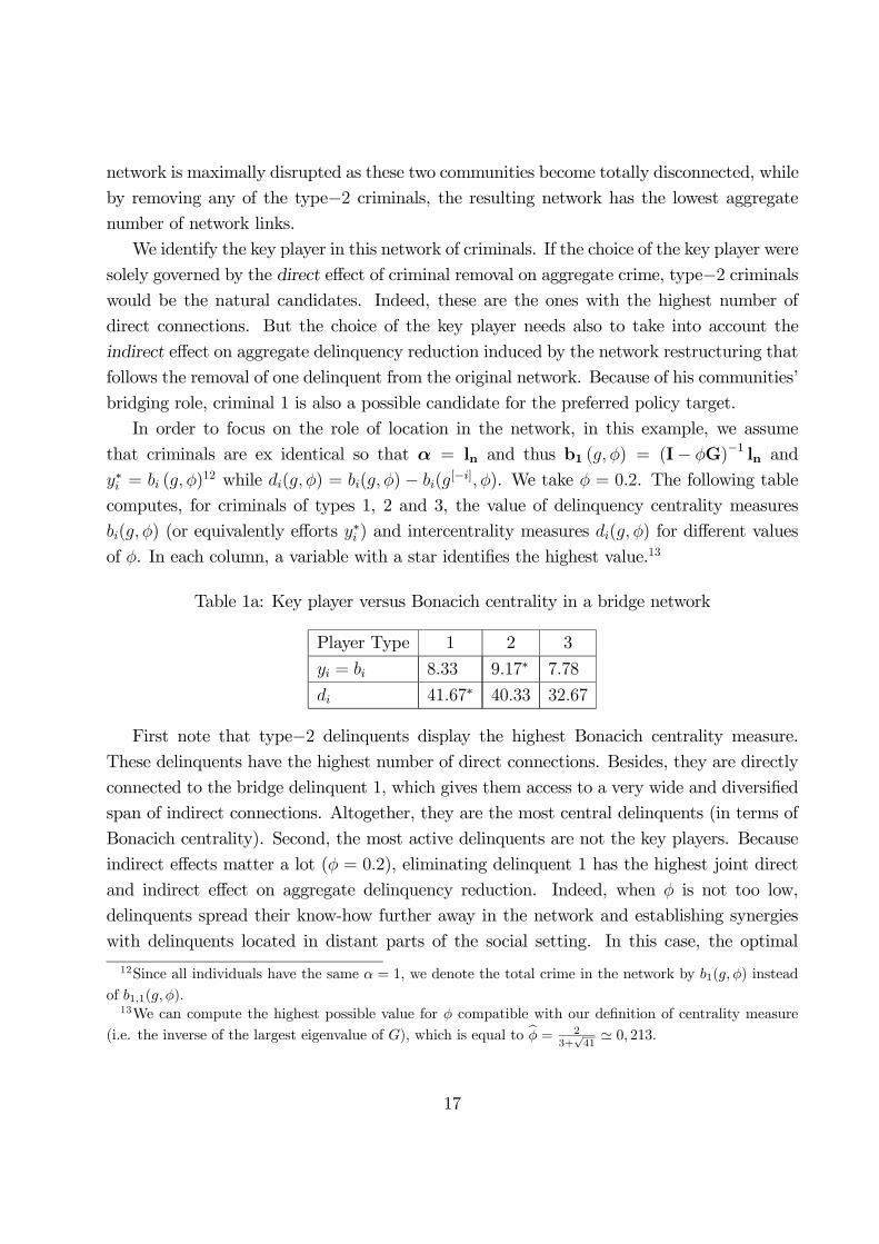
In order to focus on the role of location in the network, in this example, we assume
that criminals are ex identical so that = ln and thus b1 ( ) = (I G) 1 ln and
= ( )12 while ( ) = ( ) ( [ ] ). We take = 0 2. The following table
computes, for criminals of types 1, 2 and 3, the value of delinquency centrality measures
( ) (or equivalently e orts ) and intercentrality measures ( ) for di erent values
of . In each column, a variable with a star identies the highest value.13
Table 1a: Key player versus Bonacich centrality in a bridge network
Player Type 1 2 3
= 8 33 9 17 7 78
41 67 40 33 32 67
First note that type 2 delinquents display the highest Bonacich centrality measure.
These delinquents have the highest number of direct connections. Besides, they are directly
connected to the bridge delinquent 1, which gives them access to a very wide and diversied
span of indirect connections. Altogether, they are the most central delinquents (in terms of
Bonacich centrality). Second, the most active delinquents are not the key players. Because
indirect e ects matter a lot ( = 0 2), eliminating delinquent 1 has the highest joint direct
and indirect e ect on aggregate delinquency reduction. Indeed, when is not too low,
delinquents spread their know-how further away in the network and establishing synergies
with delinquents located in distant parts of the social setting. In this case, the optimal
12Since all individuals have the same = 1, we denote the total crime in the network by 1( ) insteadof 1 1( ).13We can compute the highest possible value for compatible with our denition of centrality measure
(i.e. the inverse of the largest eigenvalue of ), which is equal to b = 23+ 41
' 0 213
17
targeted policy is the one that maximally disrupts the delinquency network, thus harming
the most its know-how transferring ability.
In Table 1a, we have shown that the key player is not the most active criminal (i.e. does
have the highest Bonacich centrality). To further understand this result, let us analyze the
characteristics of all criminals in terms of network position, as well as those of the network
described in Figure 3. For that, we will rst use some measures of centrality other than
Bonacich. Indeed, over the past years, social network theorists have proposed a number of
centrality measures to account for the variability in network location across agents (Wasser-
man and Faust, 1994).14 While these measures are mainly geometric in nature, our theory
provides a behavioral foundation to the Bonacich centrality measure (and only this one)
that coincides with the unique Nash equilibrium of a non-cooperative peer e ects game on
a social network. Let us now calculate for the network given in Figure 3 the other individ-
ual centrality measures, namely: degree, closeness, betweenness centralities as well as the
clustering coe cient. Their mathematical denitions are given in Appendix 4. We obtain:
Table 1b: Characteristics of criminals in a network
where the most active criminal is not the key playerPlayer type 1 2 3
Degree centrality 0.4 0.5 0.4
Closeness centrality 0.625 0.555 0.416
Betweenness centrality 0.555 0.2 0
Clustering coe cient 0.33 0.7 1
Even if player 1 is not the most active criminal (she has the lowest degree centrality
and the lowest clustering coe cient), it is now even easier to understand why she is the key
player: she has the highest closeness and betweenness centralities. Observe that criminal 3
has a betweenness centrality equals to zero because there are no shortest path between two
criminals that go through her.
Let us now examine the characteristics of the network described in Figure 3 where the
key player is not the most active criminal. We will consider standard network characteristics,
which are all dened in Appendix 4. We obtain the following results:
14See Borgatti (2003) for a discussion on the lack of a systematic criterium to pick up the �“right�” networkcentrality measure for each particular situation.
18
Table 1c: Characteristics of the network
in which the most active criminal is not the key playerNetwork Characteristics
Average Distance 2.11
Average Degree 4.36
Diameter 4
Density 0.211
Asymmetry 0.125
Clustering 0.805
Degree centrality 7 78× 10 3
Closeness centrality 0.323
Betweenness Centrality 0.47556
Assortativity 3 49× 10 16
We see from Table 1c that the network described in Figure 3 has a low average distance
and low diameter (small-world properties), a very high clustering (0.805) and a weak dissor-
tativity. Furthermore, it is not very dense nor asymmetric while having average values of
centralities measures.
To summarize, the individual Nash equilibrium e orts of the delinquency-network game
are proportional to the equilibrium Bonacich centrality network measures, while the key
player is the delinquent with the highest intercentrality measure. As the previous example
illustrates, these two measures need not to coincide. This is not surprising, as both mea-
sures di er substantially in their foundation. Whereas the equilibrium-Bonacich centrality
index derives from strategic individual considerations, the intercentrality measure solves the
planner�’s optimality collective concerns. In particular, the equilibrium Bonacich centrality
measure fails to internalize all the network payo externalities delinquents exert on each
other, while the intercentrality measure internalizes them all. More formally, the measure
( ) goes beyond the measure b ( ) by keeping track of all the cross-contributions
that arise between its coordinates 1( ) ( ).
19
4 Data description
Our analysis is made possible by the use of a unique database on friendship networks from
the National Longitudinal Survey of Adolescent Health (AddHealth).15
The AddHealth database has been designed to study the impact of the social environment
(i.e. friends, family, neighborhood and school) on adolescents�’ behavior in the United States
by collecting data on students in grades 7-12 from a nationally representative sample of
roughly 130 private and public schools in years 1994-95. Every pupil attending the sampled
schools on the interview day is asked to compile a questionnaire (in-school data) contain-
ing questions on respondents�’ demographic and behavioral characteristics, education, family
background and friendship. This sample contains information on roughly 90,000 students.
A subset of adolescents selected from the rosters of the sampled schools, about 20,000 indi-
viduals, is then asked to compile a longer questionnaire containing more sensitive individual
and household information (in-home and parental data). Those subjects of the subset are
interviewed again in 1995�—96 (wave II), in 2001�—2 (wave III), and again in 2007-2008 (wave
IV).16 For the purposes of our analysis, we focus on wave I because the network information
is only available in the rst wave.
From a network perspective, the most interesting aspect of the AddHealth data is the
information on friendships. Indeed, the friendship information is based upon actual friends
nominations. Pupils were asked to identify their best friends from a school roster (up to ve
males and ve females).17 We assume that friendship relationships are reciprocal, i.e. a link
exists between two friends if at least one of the two individuals has identied the other as
his/her best friend.18 By matching the identication numbers of the friendship nominations
to respondents�’ identication numbers, one can obtain information on the characteristics of
nominated friends. More importantly, one can reconstruct the whole geometric structure
15This research uses data from Add Health, a program project designed by J. Richard Udry, Peter S. Bear-
man, and Kathleen Mullan Harris, and funded by a grant P01-HD31921 from the National Institute of ChildHealth and Human Development, with cooperative funding from 17 other agencies. Special acknowledgmentis due Ronald R. Rindfuss and Barbara Entwisle for assistance in the original design. Persons interestedin obtaining data les from Add Health should contact Add Health, Carolina Population Center, 123 W.Franklin Street, Chapel Hill, NC 27516-2524 ([email protected]). No direct support was received fromgrant P01-HD31921 for this analysis.16The AddHealth website describes survey design and data in details.
http://www.cpc.unc.edu/projects/addhealth17The limit in the number of nominations is not binding (even by gender). Less than 1% of the students
in our sample show a list of ten best friends.18We considered non-reciprocal friendship networks below.
20
of the friendship networks. For each school, we thus obtain all the network components of
(best) friends.19
The in-home questionnaire contains an extensive set of questions on juvenile delinquency,
that are used to construct our dependent variable. Specically, the AddHealth contains
information on 15 delinquency items.20 The survey asks students how often they participate
in each of these activities during the past year.21 Each response is coded using an ordinal
scale ranging from 0 (i.e. never participate) to 1 (i.e. participate 1 or 2 times), 2 (participate
3 or 4 times) up to 3 (i.e. participate 5 or more times). To derive quantitative information
on a topic using qualitative answers to a battery of related questions, we calculate an index
of delinquency involvement for each respondent.22 It ranges between 0.09 and 9.63, with
mean equal to 0.94 and standard deviation to 1.09.
Because of the theoretical model (Section 3), we focus only on networks of delinquents,
thus excluding the individuals who report never participating in any delinquent activity
(roughly 40% of the total). Also, we do not consider networks at the extremes of the
network size distribution to avoid the possibility that in these edge networks the strength of
peer e ects as well as the removal of the key player can have extreme values (too low or too
high) that may be a matter of concern. Excluding individuals with non valid information,
we obtain a nal sample of 1,297 criminals distributed over 150 networks. The minimum
number of individuals in a delinquent network is 4 while its maximum is 77. The mean and
the standard deviation of network size are roughly 9 and 12 pupils, respectively.23
19Note that, when an individual identies a best friend who does not belong to the same school, thedatabase does not include in the network of ; it provides no information about . Fortunately, in the largemajority of cases (more than 93%), best friends tend to be in the same school and thus are systematicallyincluded in the network.20Namely, paint gra ti or signs on someone else�’s property or in a public place; deliberately damage
property that didn�’t belong to you; lie to your parents or guardians about where you had been or whom youwere with; take something from a store without paying for it; get into a serious physical ght; hurt someonebadly enough to need bandages or care from a doctor or nurse; run away from home; drive a car without itsowner�’s permission; steal something worth more than $50; go into a house or building to steal something; use
or threaten to use a weapon to get something from someone; sell marijuana or other drugs; steal somethingworth less than $50; take part in a ght where a group of your friends was against another group; act loud,rowdy, or unruly in a public place.21Respondents listened to pre-recorded questions through earphones and then they entered their answers
directly on laptop computers. This administration of the survey for sensitive topics minimizes the potentialfor interview and parental inuence, while maintaining data security.22This is a standard factor analysis, where the factor loadings of the di erent variables are used to derive
the total score.23On average, delinquents declare having 2.26 delinquent friends with a standard deviation of 1.52.
21
Table A.1 in Appendix 1 provides the descriptive statistics and denitions of the variables
used in our study.24 Among the adolescents selected in our sample of delinquents, 32% are
female and 19% are blacks. An average, criminal adolescent feel that adults care about
them but have some trouble getting along with the teachers. Slightly less than 70% of our
adolescents live in a household with two married parents, although about 30% come from a
single parent family. The most popular occupation of the father is a manual one (roughly
30%) and 17% of them have parents who works in a professional/technical occupation. The
average parental education is high school graduate. Almost 40% of our adolescents live in
suburban areas. The performance at school, as measured by the mean mathematics score
is slightly above the average. On average, our criminals consider themselves slightly more
intelligent than their peers and their level of physical development appear to be slightly
higher when compared to other boys/girls of the same age.25 Our analysis in the following
sections will shed lights on the characteristics of the most harmful individuals, that is on
those pupils that, if removed, would lead to the highest crime reduction in their own groups.
5 Peer e ects and network centrality
Let us now begin the test of our theoretical framework (Section 3) by providing an appropri-
ate estimate of peer e ects in crime (b). We rst present our empirical model and estimationstrategy. We use the architecture of networks to identify peer e ects as described in Bra-
moullé et al. (2009) and Lee et al. (2010) but we consider the case of a non-row-normalized
G and we highlight the methodological improvements that are achieved in our context. Our
estimation method follows the 2SLS and GMM strategies proposed by Lee (2007) and rened
by Liu and Lee (2010) to capture the impact of centrality in networks. To be more specic,
we will begin by explaining the empirical issues than hinder the identication of peer e ects
and show to what extent it is possible to tackle each of these issues with the AddHealth
dataset.24Information at the school level, such as school quality and teacher/pupil ratio, is unnecessary given our
xed e ects estimation strategy.25When reading these summary information, one need to keep in mind that we deal here with juvenile
delinquency, where some of the o ences recorded as crimes (such as paint gra ti or lie to the parents) arequite minor.
22
5.1 Empirical model
Let ¯ be the total number of networks in the sample (150 in our dataset), be the number of
individuals in the th network, and =P¯
=1 be the total number of sample observations.
Dening the ex ante heterogeneity of each individual in network as
= 0 +1 P
=1
0
the empirical model corresponding to (4) can be written as:
=P=1
+ 0 +1 P
=1
0 + + (11)
for = 1 · · · and = 1 · · · ,̄ where = ( 1 · · · )0, = , =P
=1
and �’s are i.i.d. innovations with zero mean and variance 2 for all and .
5.2 Identication strategy
The identication of peer e ects ( in model (11)) raises di erent challenges.
Reection problem In linear-in-means models, simultaneity in behavior of interacting
agents introduces a perfect collinearity between the expected mean outcome of the group and
its mean characteristics. Therefore, it is di cult to di erentiate between the e ect of peers�’
choice of e ort and peers�’ characteristics that do impact on their e ort choice (the so-called
reection problem; see Manski, 1993). Basically, the reection problem arises because, in
the standard approach, individuals interact in groups, that is individuals are a ected by
all individuals belonging to their group and by nobody outside the group. In other words,
groups completely overlap. In the case of social networks, instead, this is nearly never true
since the reference group has individual-level variation. Take individuals and such that
= 1. Then, individual is directly inuenced byP
=1 while individual is directly
inuenced byP
=1 , and there is little chance for these two values to be the same unless
the network is complete (i.e. everybody is linked with everybody). Formally, as shown by
Bramoullé et al. (2009), social e ects are identied (i.e. no reection problem) if I, G and
G2 are linearly independent, where G2 keeps track of indirect connections of length 2 in .26
26For example, complete networks do not satisfy this condition. In our dataset, where 150 networks areconsidered (see above in the data section), many of them have di erent sizes but none of them are completeand all satisfy the condition that guarantees the identication of social e ects. Note that, even when networksare all complete, Lee (2007) shows that identication can be achieved by exploring strengths of interactionsacross networks of di erent sizes.
23
In other words, if and are friends and and are friends, it does not necessarily imply that
and are also friends. Because of these intransitivities, G2x G3x etc. are not collinear
with Gx and they act as valid instruments for Gy (under the situation that x is relevant).
Intuitively, G2x represents the vector of the friends�’ friends attributes of each agent in the
network. The architecture of social networks implies that these attributes will a ect her
outcome only through their e ect on her friends�’ outcomes. Even in linear-in-means models
the Manski�’s (1993) reection problem is thus eluded.27 Peer e ects in social networks are
thus identied and can be estimated using 2SLS (Lee 2007; Lin, 2010). In Appendix 2 we
detail in a more technical way the identication of model (11). In particular, we highlight
the di erence between the case with row-normalizedG (Bramoullé et al., 2009) and our case
with non-row-normalized G.
Endogenous network formation/correlated e ects Although this setting allows
us to solve the reection problem, the estimation results might still be awed because of the
presence of unobservable factors a ecting both individual and peer behavior. It is indeed
di cult to disentangle the endogenous peer e ects from the correlated e ects, i.e. from e ects
arising from the fact that individuals in the same network tend to behave similarly because
they face a common environment. If individuals are not randomly assigned into networks,
this problem might originate from the possible sorting of agents. If the variables that drive
this process of selection are not fully observable, potential correlations between (unobserved)
network-specic factors and the target regressors are major sources of bias. Observe that our
particularly large information on individual (observed) variables should reasonably explain
the process of selection into groups. However, a number of papers have treated the estimation
of peer e ects with correlated e ects (e.g., Clark and Loheac 2007; Lee 2007; Lin 2010; Lee
et al. 2010). This approach is based on the use of network xed e ects and extends Lee
(2003) 2SLS methodology after the removal of network xed e ects. Network xed e ects
can be interpreted as originating from a two-step model of link formation where agents
self-select into di erent networks in a rst step with selection bias due to specic network
characteristics and, then, in a second step, link formation takes place within networks based
on observable individual characteristics only. An estimation procedure alike to a panel within
group estimator is thus able to control for these correlated e ects. One can get rid of the
27These results are formally derived in Bramoullé et al. (2009) (see, in particular, their Proposition 3) andused in Calvó-Armengol et al. (2009) and Lin (2010). Cohen-Cole (2006) presents a similar argument, i.e.the use of out-group e ects, to achieve the identication of the endogenous group e ect in the linear-in-meansmodel (see also Weinberg et al., 2004; Laschever, 2009). See Durlauf and Ioannides (2010) and Blume et al.(2011) for an overview on these issues.
24
network xed e ects by subtracting the network average from the individual-level variables.28
As detailed in the next section, this paper follows this approach.
Specic individual and contextual e ects In this respect, the richness of the in-
formation provided by the AddHealth questionnaire on adolescents�’ behavior allow us to
nd observable individual variables as well as proxies for typically unobserved individual
characteristics that may be correlated with our variable of interest. Specically, to control
for di erences in leadership propensity across adolescents, we include an indicator of self-
esteem and an indicator of the level of physical development compared to the peers, and we
use mathematics score as an indicator of ability. Also, we attempt to capture di erences
in attitude towards education, parenting and more general social inuences by including
indicators of the student�’s school attachment, relationship with teachers, parental care and
social inclusion.
To summarize, our identication strategy is based on the assumption that any troubling
source of heterogeneity (if any), which is left unexplained by our unusually large set of
observed characteristics can be captured at the network level, and thus taken into account
by the inclusion of network xed e ects.
To be more precise, we allow link formation (as captured by our matrix G) to be corre-lated with observed individual characteristics,29 contextual e ects (G x, where G is row-
normalized from G) and unobserved network characteristics (captured by the network xed
e ects). The presence of other remaining unobserved e ect is very unlikely in our case given
our set of controls that includes behavioral factors and, most importantly, because we deal
with quite small networks (see Section 4).
Deterrence e ects So far, we have dealt with issues that are common to the identi-
cation of any kind of peer e ects. There is, however, something that is specic to crime:
How deterrence e ects ( in our theoretical model) are measured? The identication of de-
terrence e ects on crime is an equally di cult empirical exercise because of the well-known
potential simultaneity and reverse causality issues (Levitt, 1997), which cannot be totally
solved using our network-based empirical strategy. Network xed e ects also prove useful in
this respect. Because in our sample, networks are within schools, the use of network xed
e ects also accounts for di erences in the strictness of anti-crime regulations across schools
28Bramoullé et al. (2009) also deal with this problem in the case of a row-normalized G matrix. In theirProposition 5, they show that if the matrices I, G, G2 and G3 are linearly independent, then by subtractingfrom the variables the network average social e ects are again identied and one can disentangle endogenouse ects from correlated e ects. In our dataset this condition of linear independence is always satised.29As long as the link formation process between two individuals does not involve the characteristics of any
third individual (see Sections 3.3). This assumption is subject to a diagnostic test below (Section 6.2).
25
(i.e. di erences in the expected punishment for a student who is caught possessing illegal
drug, stealing school property, verbally abusing a teacher, etc.). As mentioned above, they
account for any kind of school level heterogeneity. As a result, instead of directly estimating
deterrence e ects (i.e. to include in the model specication observable measures of deter-
rence, such as local police expenditures or the arrest rate in the local area), we focus our
attention on the estimation of peer e ects in crime, accounting for network xed e ects.
5.3 Econometric methodology
Let yr = ( 1 · · · )0, xr = ( 1 · · · )0, and ²r = ( 1 · · · )0. Denote the
× sociomatrix by Gr = [ ], the row-normalized Gr by Gr, and an -dimensional
vector of ones by ln . Then model (11) can be written in matrix form as:
yr = Gryr + xr + ln + ²r
where xr = (xr Grxr) and = ( 0 0)0.
For a sample with ¯ networks, stack up the data by dening y = (Y01 · · · Y0
where D(A1 · · · AK) is a block diagonal matrix in which the diagonal blocks are ×matrices Ak�’s. For the entire sample, the model is
y = z + · + ² (12)
where z = (Gy x ) and = ( 0)0.
We treat as a vector of unknown parameters. When the number of networks ¯ is large,
we have the incidental parameter problem. Let J = D(J1 · · · Jr̄), where Jr = In 1 ln l0n .
The network xed e ect can be eliminated by the transformation J such that
Jy = Jz + J² (13)
LetM = (I G) 1. The equilibrium outcome vector y in (12) is given by the reduced
form equation
y =M(x + · ) +M² (14)
It follows thatGy = GMx +GM +GM². Gy is correlated with because E[(GM²)0²] =2tr(GM) 6= 0. Hence, in general, (13) cannot be consistently estimated by OLS.30 If G
30Lee (2002) has shown the OLS estimator can be consistent in the spatial scenario where each spatialunit is inuenced by many neighbors whose inuences are uniformly small. However, in the current data,the number of neighbors are limited, and hence that result does not apply.
26
is row-normalized such that G · ln = ln, the endogenous social interaction e ect can be
interpreted as an average e ect. With a row-normalized G, Lee et al. (2010) have proposed
a partial-likelihood approach for the estimation based on the transformed model (13). How-
ever, for this empirical study, we are interested in the aggregate endogenous e ect instead of
the average e ect. Hence, row-normalization is not appropriate. Furthermore, we are also
interested in the centrality of networks that are captured by the variation in row sums (out-
degrees) in the adjacency matrix G. Row-normalization could eliminate such information.
However, asG is not row-normalized in this empirical study, the (partial) likelihood function
for (13) could not be derived, and alternative estimation approaches need to be considered.
In this paper, we estimate (13) by the 2SLS and generalized method of moments (GMM)
approaches proposed by Liu and Lee (2010). The conventional instrumental matrix for the
estimation of (13) is Q1 = J(Gx x ) (nite-IVs 2SLS). For the case that the adjacency
matrix G is not row-normalized, Liu and Lee (2010) have proposed to use additional in-
struments (IVs) JG so that QK = (Q1 JG ) (many-IVs 2SLS). The additional IVs JG
are based on the row sums of G and thus use the information on centrality of a network.
Those additional IVs could help model identication when the conventional IVs are weak
and improve upon the estimation e ciency of the conventional 2SLS estimator based on
Q1. The number of such instruments depends on the number of networks. If the number
of networks grows with the sample size, so does the number of IVs. The 2SLS could be
asymptotic biased when the number of IVs increases too fast relative to the sample size (see,
e.g., Bekker, 1994; Bekker and van der Ploeg, 2005; Hansen et al., 2008). Liu and Lee (2010)
have shown that the proposed many-IV 2SLS estimator has a properly-centered asymptotic
normal distribution when the average group size needs to be large relative to the number of
networks in the sample. As detailed in Section 4, in this empirical study, we have a number
of small networks. Liu and Lee (2010) have proposed a bias-correction procedure based
on the estimated leading-order many-IV bias. The bias-corrected many-IV 2SLS estimator
(bias-corrected 2SLS) is properly centered, asymptotically normally distributed, and e cient
when the average group size is su ciently large. It is thus the more appropriate estimator
in our case study.
The 2SLS approach can be generalized to the GMM with additional quadratic moment
equations (nite-IVs GMM, many-IVs GMM ). While the IV moments use the information
of the main regression function of (14) for estimation, the quadratic moments explore the
correlation structure of the reduced form disturbances. Liu and Lee (2010) have shown
that the many-IV GMM estimators can be consistent, asymptotically normal, and e cient
when the sample size grows fast enough relative to the number of networks. Liu and Lee
27
(2010) have also suggested a bias-correction procedure for the many-IV GMM estimator
based on the estimated leading order many-instrument bias. The bias-corrected many-IV
GMM estimator (bias-corrected GMM ) is shown to be more e cient than the corresponding
2SLS estimator. Appendix 3 details the derivation and asymptotic properties of both the
2SLS and GMM estimators.
5.4 Estimation results
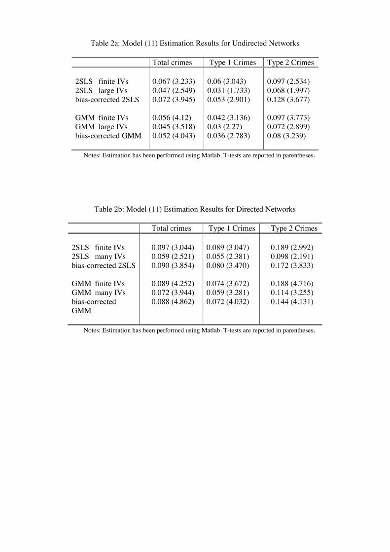
Table 2a collects the estimation results of model (11) when using the di erent estimators
discussed in the previous section.
As explained above, for the estimation of , we pool all the networks together by con-
structing a block-diagonal network matrix with the adjacency matrices from each network on
the diagonal block. Hence we implicitly assume that the in the empirical model is the same
for all networks. The di erence between networks is controlled for by network xed e ects.
Indeed, the estimation of for each network might be di cult (in terms of precision) for
the small networks. Furthermore, it is a crucial empirical concern to control for unobserved
network heterogeneity by using network xed e ects.
For equation (6) to be well-dened, needs to be in absolute value smaller than the
inverse of the largest eigenvalue of the block-diagonal network matrix (Proposition 1). In
our case, the largest eigenvalue of G is 5 59. Furthermore our theoretical model postulates
that 0 As a result, we can accept values within the range [0 0 179). Table 2 shows
that all our estimates of are within this parameter space. As explained above, in our case
study with small networks in the sample, the preferred estimator is the bias-corrected one.
The GMM generalization improves upon the precision of the 2SLS estimates. Let us thus
focus on the bias-corrected many-IV GMM estimator and interpret the results in terms of
magnitude. We nd that a standard deviation increase in the aggregate level of delinquent
activity of the peers translate into a roughly 11 percent increase of a standard deviation
in the individual level of activity. This is a strong e ect, especially given our long list of
controls.
[ 2 ]
5.5 Directed networks
So far, we have only considered undirected networks, i.e. we have assumed that friendship
relationships are reciprocal, = . Our data, however, make it possible to know exactly
28
who nominates whom in a network. Indeed, 20 percent of relationships in our dataset are
not reciprocal.
In order to see how robust is our analysis, we now exploit the directed nature of the
network data. Of course, the interpretation of centrality is now di erent since centrality
contributions only ow in one direction on the directed links. We would like to see if our
results change signicantly under such a specication.
We follow the approach of Wasserman and Faust (1994, pages 205-210) who dene the
Katz-Bonacich centrality measure for directed networks. As they put it: �“Centrality indices
for directional relations generally focus on choices made�”.
In the language of graph theory, in a directed graph, a link has two distinct ends: a
head (the end with an arrow) and a tail. Each end is counted separately. The sum of
head endpoints count toward the indegree and the sum of tail endpoints count toward the
outdegree. Formally, we denote a link from to as = 1 if has nominated as his/her
friend, and = 0, otherwise. The indegree of student , denoted by + , is the number of
nominations student receives from other students, that is + =P
. The outdegree of
student , denoted by , is the number of friends student nominates, that is =P
.
We consider only the indegree to dene the Katz-Bonacich centrality measure. Observe that,
by denition, the adjacency matrix G = [ ] is now asymmetric.
In the empirical analysis, we use outdegrees because if individual nominates but
does not, it is then very possible that is a role model for . In other words, is learning
from even though does not consider as his/her best friend. In this context, , the
criminal activities of , inuences .
From a theoretical point of view, the symmetry of G does not play any explicit role for
the result established in Proposition 1. We can therefore dene the Katz-Bonacich centrality
measure b ( ) exactly as in (3).
Turning to the empirical analysis, Table 2b reports the results of the estimation of model
(11) when the directed nature of the network data is taken into account (i.e., with this
alternative specication of G). The parameter space [0 1 1(G)) is [0 0 322). Table 2b
shows that the estimates of are all within this range. They are still statistically signicant
and only slightly higher in magnitude. Therefore, the results do not change substantially.
[ 2 ]
29
6 Who is the key player? Counterfactural Study
Let us now calculate empirically who is the key player in each our real-world networks. We
set out a counterfactual study, which is now described.
6.1 Description of the procedure
With the estimates obtained from the bias-corrected many-IV GMM estimation procedure,
for a network , r = Grxr + xr + rln + ²r can be estimated by
�ˆr = (In �ˆGr)yr
As b r( ) = (In �ˆGr)1�ˆr = yr, the × 1 vector of Bonacich centrality of network
is given by yr. As a result, the initial level of aggregate crime e ort is given by:
bsr( ) = l0n (In
�ˆGr)1�ˆr = l
0n yr
To identify the key player, we proceed exactly as in the theoretical model (see Section 3.2).
For that, we calculate the crime reduction for removal of each player, one at a time, in
the network. The key player is the one associated with the largest crime reduction. Let
�ˆer = (In �ˆGr)yr Grxr�ˆ. When a player is removed, we drop the th row of xr and
�ˆer to get exr and �˜er, and drop the th row and column of Gr to get �˜Gr. Let �˜Gr be the
row-normalized �˜Gr. Then the aggregate crime e ort with a player being removed is
bsr( [ ] ) = l0n (In 1
�ˆ �˜Gr)1(�˜Grexr�ˆ + �˜er) = l0n eyr
where eyr is the vector of criminal activities in network when the criminal has been
removed.31 As in the theoretical model (see (8)), the key player is given by:
argmax(bsr( ) bs
r( [ ] )) = argminbs
r( [ ] ) (15)
6.2 The invariant assumption on [ ]: Empirical issues
As observed in Section 3.2, in the calculation of the key player (in the formula (8) or,
equivalently, in the simulations (15)), it is assumed that, when the key player is removed,
31Note that in this exercise the predicted Bonacich centralities and crime rates are the same because thedenition of in equation (6) ( = + + ) includes the xed-network e ects ( ) andthe error term . A less tractable set up where the equality is not necessarily true would imply to replaceby in equation (6).
30
the other criminals in the network do not form new links (i.e. invariance of [ ], i.e. network[ ] has adjacency matrix G[ ] where the th row and the th column have been removed
from G). In Section 3.3, we propose a simple network formation model that could justify
this assumption. In this model, the link between and in network only depends in the
observable characteristics of and but not on the characteristics of the other criminals in
the network (including �’s friends other than ). In this section, we would like to test this
model with our data.
Let us rst consider undirected networks. For a network with criminals, if G is
undirected, we have ( 1) 2 distinct links in the network. Consider the following model:
= | | +
µmin6=| |
¶1 +
µmin6=| |
¶2 + + (16)
for = 1 · · · 1, = + 1 and = 1 · · · ,̄ and where the notations are the
same as for model (11). Our aim is to test the hypothesis that 1 = 2 = 0, that is the link
between and does not depend on individual (whether is a direct friend of or not).
For directed networks, for a network with criminals, if G is directed, we have
( 1) distinct links in the network and we test the following model:
= | | +
µmin6=| |
¶+ + (17)
for = 1 · · · , 6= and = 1 · · · ,̄ and where the notations are the same as for
model (11). We will test here the hypothesis that = 0.
Here, we do not claim any causality. We are just looking at correlations and see if the
network formation model proposed in Section 3.3 would not be rejected by the data. This
is just a diagnostic check.
A linear probability model is estimated via least squares with network xed e ects. Ta-
bles 3a and 3b display the estimation results for the undirected and directed networks,
respectively. It is clear from these tables that, for most variables, the formation of a link
(i.e. friendship) between two criminals and is primarily a ected by the observable char-
acteristics of and but not by the characteristics of any other criminal 6= belonging
to the same network, that is, is signicant while (or 1 and 2 in the case of undirected
networks) is not. Furthermore, since the sign of is nearly always negative, there seems to
be homophily in the friendship formation in these criminal networks, that is the closer two
persons are in terms of characteristics, the more likely they will be friends.
[ 3 3 ]
31
6.3 Individual characteristics of key players
Once we have identied the key player for each network, we can draw his/her �“prole�” by
comparing the characteristics of these key players with those of the other criminals in the
network.32 Table 4 displays the results only for the variables whose di erences in means
between these two samples are statistically signicant. Compared to other criminals, �“key�”
criminals belong to families whose parents are less educated and have the perception of being
socially more excluded. They also feel that parents care less about them and have more
troubles getting along with the teachers. Furthermore, the typical key player is more likely
to be a male and have friends who are older and less attached to religion than other criminals.
He/she is also more likely to come from residential areas with industrial properties of various
types, although her/his friends are less likely to come from these kind of neighborhoods.
Table A.2 in Appendix 4 contains the summary statistics of all the characteristics of the key
players, as well as the ones of their best friends.
[ 4 ]
An interesting and important question that we seek to investigated empirically is whether
the key player is always the player with the highest crime level (or equivalently with the
highest Bonacich centrality in the network). We have shown in theoretical section that, in
some cases, it is not the case (see Section 3.4) because the two measures (Bonacich versus
inter-centrality) di er substantially in their foundation. Whereas the equilibrium-Bonacich
centrality index (dened in (3)) derives from strategic individual considerations, the inter-
centrality measure (dened in (8)) solves the planner�’s optimality collective concerns. In
particular, the equilibrium Bonacich centrality measure fails to internalize all the network
payo externalities delinquents exert on each other, while the intercentrality measure inter-
nalizes them all.
For each of our 150 networks, we investigate whether the key player is also the most
active criminal in the network (i.e. has the highest Bonacich centrality). We nd that in
40 out of 150 networks (27%), it is not the case. This interesting (and unexpected) result
is important for policy purposes since it means that, in some cases, we should not always
target the most active criminals in a network.
In Table 5, we compare the characteristics of key players who are the most active crimi-
nals in the network with key players who are not. As in Table 4, Table 5 only shows variables
32Since the results on key players for directed networks are relatively similar, we will not discuss them.They are available upon request.
32
whose di erences in means between these two samples are statistically signicant. As com-
pared to other key players, we nd that key players who are not the most active criminals are
more attached to religion,33 are less likely to have single parents, to be socially integrated and
have less troubles getting along with your teachers. They are also less physically developed
and are less �“able�” individuals (to the extent to which mathematics score is a good proxy
for individual ability). Now, looking at di erences in the characteristics of their friends, it
appears that key players who are not the most active criminals in the network have friends
who have parents with higher education, who are less likely to be in manual occupations and
a higher proportion of their friends feel that parents care very much about them. Compared
to the key players who are the most active criminals in their network, their friends are also
more religious. Our ndings suggest that di erences in the family background of the friends
of key players may be important factors explaining the observed di erences in crime between
di erent types of key players. They can act as important protective factors. On the other
hand, we are not able to detect relevant di erences in neighborhood attributes to conclude
that also neighborhood quality acts as a protective factor.
[ 5 ]
6.4 Petty versus serious crimes
We would like now to investigate whether the characteristics of key players di er by types of
crime. For that, we split the reported o ences between petty crimes andmore serious crimes.
The rst group (type-1 crimes or petty crimes) encompasses the following o ences: ( ) paint
gra ti or sign on someone else�’s property or in a public place; ( ) lie to the parents or
guardians about where or with whom having been; ( ) run away from home; ( ) act loud,
rowdy, or unruly in a public place; ( ) take part in a group ght; ( ) damage properties that
do not belong to you; ( ) steal something worth less than $50. The second group (type-2
crimes or more serious crimes) consists of ( ): taking something from a store without paying
for it; ( ) hurting someone badly enough to need bandages or care from a doctor or nurse;
( ) driving a car without its owner�’s permission; ( ) stealing something worth more than
$50; ( ) going into a house or building to steal something; ( ) using or threatening to use a
weapon to get something from someone; ( ) selling marijuana or other drugs; ( ) getting
into a serious physical ght.
We obtain a sample of 1099 petty criminals distributed over 132 networks and a sample
33Note that a higher value of the variable �“Religion practice�” means in fact that the person is less religious.
33
of 545 more serious criminals distributed over 75 networks. Petty crime networks have a
minimum of 4 individuals and a maximum of 73 (with mean equals to 8.33 and standard
deviation equals to 10.74), whereas the range for more serious crime networks is between 4
and 38 (with mean equals to 7.27 and standard deviation equals to 6.64).
We estimate model (11) for di erent crime types, which provides type of crime-specic
peer e ects. The results for undirected networks are contained in the last two columns of
Table 2a. All estimates are within the acceptable parameter space [0 0 180) for type-1 crimes
and [0 0 219) for type-2 crimes. In terms of magnitude, it appears that the impact of peer
e ects on crime are much higher for more serious crimes than for petty crimes. Indeed,
we nd that a standard deviation increase in the aggregate level of delinquent activity of
the peers translate into a roughly 8 percent and 14.5 increase of a standard deviation in
the individual level of activity for petty crimes and more serious crimes, respectively. The
results for directed networks are contained in the last two columns of Table 2b. They are not
qualitatively di erent (only slightly higher in magnitude). All the estimates are within the
parameter space [0 1 1(G)) which is [0 0 322) and [0 0 423) for type-1 crimes and type-2
crimes, respectively.
We then repeat our counterfactual studies for key players for di erent types of crimes.
Although the results of this exercise need to be taken with caution because of the small
sample size of students committing the more serious o ences, we report our ndings in
Tables 6 10.34
Table 6 and 7 have the same structure as Table 4 but draw a prole of the key player
for petty and more serious crimes. As compared to other criminals, a key player committing
petty crimes is more likely to be a male, less likely to be black, is more able than other
criminals, more likely to feel that parents do not care very much about him/her and has
troubles getting along with teachers. His/her friends have parents who are less likely to be
o ce or sales workers and in the farm or shery sector. They come more frequently from
suburban areas and have less troubles getting along with the teachers than friends of other
types of criminals.
The portrait of a key player committing serious crimes has di erent features. Even
though he/she is more likely to be a male, he/she is more physically developed compared
to the boys of his/her age, feels to be part of the school but has troubles getting along
with teachers. He/she is also more likely to reside in suburban areas and less likely in urban
residential areas. Neither key players committing serious crime nor their friends have parents
34Also, in this case, we expose our results undirected networks only. The evidence for directed networks
is similar. These results are also available upon request.
34
working in the military or security sector. The typical key player committing serious crimes
has friends who are older, less likely to come from industrial residential areas and his/her
parents are less likely to be in the farm or shery sector.
[ 6 7 ]
Table 8 instead compares the characteristics of key players for di erent types of crimes.
We nd only few signicant di erences in individual characteristics while di erences in their
friends�’ characteristics seem to be more important. Key players committing serious crime
are more likely to be black and have friends who are blacks and feel that adults care about
them more than key players committing petty crimes. This last aspect is not true for their
friends. Also, as compared to friends of key players committing petty crimes, key players�’
friends in serious crimes are more able, have more troubles with teachers, are more likely
to have parents in o ce or sales occupations and less likely to have parents occupied in the
military or security sector. A larger proportion of them comes from urban residential areas.
[ 8 ]
Finally, Tables 9 and 10 have the same structure as Table 5 and uncover the di erence in
characteristics for di erent types of crimes between key players who are the most criminals
and those who are not. When the o ences are di erentiated by the type of crime committed,
we still nd some networks where the most �“harmful�” criminal is not the individual with the
highest Bonacich centrality (30% for petty crimes and 25% for serious crimes). Key players
committing petty crimes who are not the most active criminals are less physically developed
compared to more active key players, more religious and have less troubles getting along
with the teachers. Interestingly, they have also less educated parents and their parents are
less likely to be managers.
For serious crimes, the picture takes again di erent aspects. Key players in serious crimes
who are not the most active criminals are individuals coming from households with more
numerous members and are less likely to be of a race di erent from white and black. They
also come from better quality neighborhoods, are more likely to live in suburban residential
areas while their friends are more likely to reside in urban residential areas. For serious
crimes, we also nd that di erences in parenting between friend groups might be important.
Although less active key players have friends who are less likely to have two married parents
and more likely to come from single parent families, almost all of these friends feel that
parents care about them very much.
35
[ 9 10 ]
6.5 Key players and network topology
As in Section 3.4, let us now investigate the characteristics of these key players in terms of
other network centrality measures (i.e. other than Bonacich centrality).
So far, we have used the Bonacich centrality measure to capture the importance of net-
work structure. The reason is that this measure has a precise behavioral foundation, as it
stems from our theoretical model. However, it counts the number of any path connecting
one node to the others, not the optimal ones. Let us then consider two other traditional
measures of centrality in network analysis that are based on optimal paths, i.e. closeness and
betweenness centralities, and a measure of cohesion of the sub-network around each node,
i.e. the clustering coe cient. They are all dened in Appendix 4 and used in the theory
section (3.4.)
Table 11 provides information on the distributions of these measures for the key players
in our networks and compares them with the Bonacich centrality (which is equal to the crime
level of each individual). Looking at the rst measure, betweenness centrality, one can rst
notice that at least 50% of our key players has a betweenness centrality equal to zero (i.e.
the median is equal to 0), meaning that there are few shortest paths that go through them.
However, if we consider the upper tail of this distributions, that is we look at the key players
with the highest betweenness centrality, we see that a larger portion of them are key players
who are not the most active criminals. Indeed, above the 90th percentile of the distribution
of the whole sample, 10% of the key players are not the most active criminals while it is
4.5% for the key players who are the most active criminals. This nding suggests that,
even though some criminals do not commit much crime, they can be key players because
they have a crucial position in the network in terms of betweenness centrality (for example,
in the network described in Section 3.4, individual 1 who bridges two otherwise separated
networks is not the most active criminal but is the key player and has the highest betweenness
centrality). When looking at the closeness centrality, the results are quite di erent. Indeed,
plenty of key players are quite central (median equals to 0.5). We also nd that more active
key players tend to be more concentrated in the upper tail of the closeness distribution than
less active key players (11% in the upper 90% tail versus 5%). Finally, the results on the
clustering coe cient suggest that the most active criminals are more likely to operate in
tighter networks of best friends (4.5% in the upper 95% tail versus 2.5% for key players who
36
are not the most active criminals).
[ 11 ]
In Tables 12 and 13, we perform the same analysis for petty and serious crimes, respec-
tively. Interestingly, we nd that, for serious crimes, key players have high betweenness
centrality while this is less the case for petty crimes. Indeed, if we look at p75 (lower 75%
of the distribution), we see that among key players, at least 75% of them has a betweenness
centrality less than 0.05 for petty crime while, for more serious crimes, this value is 0.67.
Moreover, for petty crimes, the most active key players seem also to be the more central
ones in terms of all measures considered while, for serious crimes, the most central players
in terms of betweenness tend to be the less criminal ones. This evidence suggests that, for
serious crimes, network position is an important determinant of key players.
[ 12 13 ]
Finally, in Tables 14, 15 and 16, we investigate the role of network characteristics35
in explaining the di erences between key players who are the most active criminals and
those who are not. In terms of statistical signicance, the di erences are not pronounced.
We only nd that, for serious crimes, the average degree is signicantly higher for most-
active key players. If we only look at the qualitative evidence, then we see that, for all
crimes, the network diameter, network betweenness and the average distance are smaller
for most-active key players. An interesting suggestive result is that networks tend to be
dissortative (�“popular�” criminals are associated with less �“popular�” ones) for petty crimes
while assortative (�“popular�” criminals are associated with �“popular�” ones) for most-active
key players committing more serious crimes.
[ 14, 15 16 ]
7 Policy implications
Identifying peer e ects in crime We would like to discuss now some policy impli-
cations of our results. As noted by Manski (1993, 2000) and Mo tt (2001), it is important
to separately identify peer or endogenous e ects from contextual or exogenous e ects. This
is because endogenous e ects generate a social multiplier while contextual e ect don�’t. In
35They are all dened in Section 3.4.
37
the context of crime, this means that a special program targeting some individuals will have
multiplier e ects: the individual a ected by the program will reduce its criminal activities
and will inuence the criminal activities of his/her peers, which, in turn, will a ect the
criminal activities of his/her peers, and so on. On the other hand, if only contextual e ects
are present, then there will be no social multiplier e ects from any policy a ecting only the
�“context�” (for example, improving the quality of the teachers at school). Therefore, the
identication of these two e ects is of paramount importance for policy purposes. Another
important policy issue in the estimation of social interactions is the separation between peer
e ects and confounding e ects. Indeed, the formation of peer group is not random and indi-
viduals do select into groups of friends. It is therefore important to separate the endogenous
peer e ects from the correlated e ects (Manski, 1993), i.e. the same criminal activities may
be due to common unobservable variables (such as, for example, the fact that individuals
from the same network like bowling together) faced by individuals belonging to the same
network rather than peer e ects. This is also very important for crime policies since, for
example, if the high-crime rates are due to the fact that teenagers like to bowling together,
then obviously the implications are very di erent than if it is due to peer e ects.
The rst aim of this paper was to clearly identify the peer e ects from the contextual
a ects and from the correlated e ects. For that, we rst developed a theoretical model where
all these e ects were clearly separated. We then estimated the results of the model by using
an econometric techniques, which utilizes the structure of the network as well as network
xed e ects to identify each of these e ects. We nd that, indeed, peer e ects are important
in criminal activities for teenagers in the United States, indicating that any policy targeting
some criminals will have multiplier e ects.
Implementing key-player policies: Theoretical issues Once this has been showed,
policy issues can be seen from a di erent perspective. Indeed, in the standard crime litera-
ture without social interactions (Becker, 1968; Garoupa, 1997; Polinsky and Shavell, 2000),
punishment is seen as an e ective tool for reducing crime. But punishment is random and
not targeted to individuals that generate the highest multiplier e ects. To address this issue,
we have developed a theoretical framework where a key player has been identied. A key
player is someone that needs to be removed in order to reduce as much as possible total
crime in the network. The way a key player is calculated is precisely using the multiplier
e ects due to endogenous peer e ects. Consider the key player removal policy. Indeed, when
a delinquent is removed from network , the intercentrality measures of all the delinquents
that remain active are reduced, that is, ([ ]
) ( ), for all 6= , which trig-
38
gers a decrease in delinquency involvement for all of them. Moreover, when delinquent
is removed from the delinquency network, the corresponding ratio of aggregate delinquency
reduction with respect to the network centrality reduction is an increasing function of the
intercentrality measure ( ) of this delinquent in network (Ballester et al., 2010).
This means that the target policy displays amplifying e ects, and the gains following the
judicious choice of the key player (the one with highest intercentrality measure) go beyond
the di erences in intercentrality measures between this player and any other delinquent in
the network.
To fully assess the relevance of the key player delinquency policy, let us compare the
relative returns of a network targeted policy with that of a random target policy. For each
criminal in the crime network , dene:
( ) =( ) (
[ ])
P=1
h( ) (
[ ])i
This is the ratio of returns (in delinquency reduction) when is the selected target versus a
random selection with uniform probability for all delinquents in the network.
Denote by ( ) the average of the intercentrality measures in network , and by
d ( ) the standard deviation of the distribution of this intercentrality measures. It can
be shown that (Ballester et al., 2010):
( ) 1 +d ( )
( )
where is the key player in for a given . The relative gains from targeting the key
player instead of operating a selection at random in the delinquency network increase with
the variability in intercentrality measures across delinquents as captured by d ( ). In
other words, the key player prescription is particularly well-suited for networks that display
stark location asymmetries across nodes. In these cases, it is more likely than the relative
gains from implementing such a policy compensate for its relative costs.
The second aim of this paper was precisely to determine the key player in each of our
adolescent networks. Because of its multiplier e ects, it is important to know what are
his/her characteristics, to which network does he/she belongs and if he/she has a di erent
prole for di erent types of crime. We nd that, compared to other criminals, key players
are more likely to be a male, have less educated parents, are less attached to religion and feel
socially more excluded. They also feel that adults care less about them, are less attached
to their school and have more troubles getting along with the teachers. We also nd that,
39
even though some criminals are not very active in criminal activities, they can be key players
because they have a crucial position in the network in terms of betweenness centrality.
Implementing key-player policies: Real-world issues How can we implement a
key-player policy? There is a small literature that discussed and tested policies aiming at
�“neutralizing�” disruptive kids because of negative peer interaction e ects they have on other
kids. Lazear (2001) proposed a model showing that class size can be an issue if some kids
are disruptive. Indeed, classroom education has public good aspects. The technology is such
that when one student disrupts the class, learning is reduced for all other students. Neither
the student nor the classmates can learn much when the student is misbehaving, causing the
teacher to allocate her time to him. The model implies that better students are optimally
placed in the large classes, despite the reduced teacher-student ratio. Using our model, we
could dene the key player as the most disruptive student in a classroom, i.e., the student
who once removed generates the highest possible increase in total education activity (as
measured by the grades of the students). �“Removing�” the key player would mean here to
put this student in another class or investing special resources (like having an extra teacher)
on him. If we follow Lazear�’s theory, it would be optimal to have �“key players�” in classes of
smaller size. Our theory helps determine who is the key player by using our intercentrality
measure while our empirical analysis helps identify the characteristics of the key player.
It is often suggested that one way to reduce juvenile crime is to lengthen the school day
or school year and/or to provide activities for young people when school is not in session.
The implicit notion behind such program-oriented solutions to juvenile crime is a belief in
the importance of incapacitation that, as Jacob and Lefgren (2003) put it: �“idle hands are
the devil�’s workshop�” and that keeping kids busy will keep them out of trouble. Advocates
of after-school and other youth programs frequently claim that juvenile violence peaks in the
after-school hours on school days and in the evenings on nonschool days. Using exogenous
policy changes and other events that e ectively force students to stay in school or take extra
days o (e.g. changes in compulsory schooling laws, teacher in-service days and strikes), a
few recent studies have shown that school attendance a ects crime in rich and complex ways.
Forcing some students to stay in school an extra year or two reduces both violent and property
crime substantially (Anderson 2009).36 Yet, day-to-day changes in school attendance have
36Anderson�’s estimates for total arrest rates imply that a compulsory schooling age of 17 signicantlyreduces age 17 arrests by about 8% (5.4 arrests per 1,000 youth) compared to a compulsory schooling ageof 16 or less. Similarly, an age 18 compulsory schooling age signicantly reduces arrests by 9.7- 11.5% atages 16-18. Overall, the estimates generally suggest that forcing youth to spend an extra year or two in highschool signicantly reduces their arrest rates over that period.
40
opposing e ects on violent and property crime. An extra day of school appears to reduce
property crime while increasing violent crime (Jacob and Lefgren, 2003; Luallen 2006).37
The latter most likely reects social interaction e ects from bringing together hundreds of
adolescents and letting them all loose at the same time.38
All the potential e ects of school attendance on crime are likely to be relevant to changes
in compulsory schooling, while the e ects of in-service days and teacher strikes are likely to
be limited to incapacitation and social interactions (Lochner, 2011). Any social interaction
e ects are likely to be magnied in the latter cases due to the universal nature of the policy.
Using our framework, we could recommend the same policies to reduce juvenile crime (i.e.
lengthen the school day or school year and/or to provide activities for young people when
school is not in session) by targeting �“key players�” instead of encompassing everybody. In
their conclusion, Jacob and Lefgren (2003) suggest that summer youth employment programs
or smaller, neighborhood-based after-school programs, that provide structured activities for
adolescents but do not substantially increase their concentration, may be the best way to
reduce juvenile crime. We could apply the same type of programs to �“key players�” that we
could identify using our framework. Targeting these �“key players�”, i.e. delinquents who once
removed generate the highest possible reduction in aggregate delinquent level in a network,
can have large e ects on crime because of the feedback e ects or �“social multipliers�” at work.
There is other strong evidence that key players matter. Two recent papers use exogenous
shocks to test the impact of �“key players�” on outcomes. Azoulay et al. (2010) look at the
impact of the sudden (i.e. prematurely and unexpected) death of 112 academic �“superstars�”
on the productivity of their co-authors. Waldinger (2010) analyzes the e ect of the expulsion
37Jacob and Lefgren (2003) examine the e ects of single day changes in school-wide attendance on juvenile
crime and arrest rates in 29 large American cities from 1995 to 1999. Exploiting teacher in-service daysacross jurisdictions over time as an exogenous source of variation in school days, they essentially comparelocal juvenile crime rates on days when school is not in session to those when it is. Their ndings suggest thatan additional day of school reduces serious juvenile property crime by about 14% that day while it increasesserious juvenile violent crime by 28%. These results are consistent with an incapacitation e ect of schoolthat limits participation in property crime. However, the increased level of interaction among adolescentsfacilitated through schools may raise the likelihood of violent conicts (and other minor delinquency) afterschool. Luallen (2006) follows a similar approach, using teacher strikes (typically lasting about 5 days)rather than in-service days as an exogenous source of school days. He nds that the incapacitation andsocial interaction e ects appear to be particularly strong in urban areas and negligible elsewhere.38Kline (2010) evaluates the e ectiveness of curfew ordinances by comparing the arrest behavior of various
age groups within a city before and after curfew enactment. The evidence suggests that curfews are e ectiveat reducing both violent and property crimes committed by juveniles below the statutory curfew age. Curfewsdo not appear to be e ective at inuencing the criminal behavior of youth just above the curfew age,suggesting that the choice of statutory curfew age is important in crafting policy.
41
of mathematics professors in Nazi Germany on PhD student outcomes. Both studies nd
strong e ects.
We believe that our key-player policy has more general policy implications and can be
applied to contexts other than crime and education. For example, the nancial market is
very connected and can be considered as a network where links could be loans between banks
(Leitner, 2005). A key-player policy would be to identify the key bank that needs to be bailed
out in order for the system to resist a nancial crisis. We could also apply the key player
policy to the issue of adoption of a new technology in developing countries. There is indeed
strong evidence of social learning (Conley and Udry, 2010). One could therefore identify key
players and target them so that their inuence on others will be crucial in the adoption of
a new technology. Another application of a key player policy could be the political world.
There is evidence that personal connections amongst politicians have a signicant impact on
the voting behavior of U.S. politicians (Cohen and Malloy, 2010). One could identify �“key
politicians�” who should be promoted within the party because they would have a signicant
impact on election outcomes.
In the real-world, howeever, we do not always have the exact information on the so-
cial network of each individual. In that case, it could be quite di cult to determine the
key player in a given network since the computation of the intercentrality measures relies
on the knowledge of the adjacency matrix of the delinquency network. This matrix is ob-
tained from sociometric data that identies the network links between delinquents.39 Our
empirical framework can help determine the key player by identifying the key and signicant
characteristics highlighted in tables 4 to 16.
Finally, we hope that the results obtained in this paper will allow policy makers to think
di erently about crime and that, in the context of nancial crisis and budget decits, there
is an alternative to �“brute force�” since targeting some specic individuals can have dramatic
e ects on crime reduction.
39Costebander and Valente (2003) show that centrality measures based on connectivity (rather than be-tweenness), such as intercentrality measures, are robust to mispecications in sociometric data, and thusopen the door to estimations of centrality measures with incomplete samples of network data. This, obvi-ously, reduces the cost of identifying the key player. The idea behind these results is that these measurestake into account all walks in the network. Thus, generally the centrality of an individual is not determinedonly by his/her direct links but by the complete structure of the network. In this sense, the probability thata missing link a ects the choice of the most central/intercentral player is smaller than with other type ofmeasures.
42
References
[1] Anderson, M. (2009), �“In school and out of trouble? The minimum dropout age and
juvenile crime,�” Unpublished manuscript.
[2] Azoulay, P., J.S. Gra Zivin and J. Wang (2010), �“Superstar extinction,�” Quarterly
Journal of Economics 125, 549-589.
[3] Ballester, C., Calvó-Armengol, A. and Y. Zenou (2006), �“Who�’s who in networks.
Wanted: the key player,�” Econometrica 74, 1403-1417.
[4] Ballester, C., Calvó-Armengol, A. and Y. Zenou (2010), �“Delinquent networks,�” Journal
of the European Economic Association 8, 34-61.
[5] Bayer, P., Hjalmarsson, R. and D. Pozen (2009), �“Building criminal capital behind bars:
Peer e ects in juvenile corrections,�” Quarterly Journal of Economics 124, 105-147.
[6] Becker, G. (1968) �“Crime and punishment: An economic approach,�” Journal of Political
Economy 76, 169-217.
[7] Bekker, P. (1994), �“Alternative approximations to the distributions of instrumental
variable estimators,�” Econometrica 62, 657-681.
[8] Bekker, P. and J. van der Ploeg (2005), �“Instrumental variable estimation based on
[71] Thornberry, T.P., Krohn, M.D., Lizotte, A.J., Smith, C.A. and K. Tobin (2003), Gangs
and Delinquency in Developmental Perspective, Cambridge: Cambridge University
Press.
[72] Verdier, T. and Y. Zenou (2004), �“Racial beliefs, location and the causes of crime,�”
International Economic Review 45, 727-756.
[73] Waldinger, F. (2010), �“Quality matters: The expulsion of professors and the conse-
quences for PhD student outcomes in Nazi Germany,�” Journal of Political Economy
118, 787-831.
[74] Warr, M. (2002) Companions in Crime: The Social Aspects of Criminal Conduct, Cam-
bridge: Cambridge University Press.
[75] Wasserman, S. and K. Faust (1994), Social Network Analysis. Methods and Applica-
tions, Cambridge: Cambridge University Press.
[76] Weinberg, B., P.B. Reagan, and J.J. Yankow (2004), �“Do neighborhoods a ect work
behavior? Evidence from the NLSY 79,�” Journal of Labor Economics 22, 891-924.
48
Appendix 1: Data appendix
Table A.1: Description of Data (1,297 individuals, 150 networks)
Variable definition Mean St.dev Min Max Delinquency index In the text 0.94 1.09 0.09 9.63 Delinquency index of best friends Aggregate value of the delinquency
index over direct friends. 2.17 2.30 0.09 20.23 Delinquency index (type-1 crime) In the text 1.15 1.15 0.20 7.31 Delinquency index of best friends (type-1 crime)
Aggregate value of the delinquency index over direct friends. 2.65 2.55 0.20 20.47
Delinquency index (type-2 crime) In the text 1.25 1.36 0.28 12.55 Delinquency index of best friends (type-2 crime)
Aggregate value of the delinquency index over direct friends. 2.57 2.48 0.28 17.52
Individual socio-demographic variables Female Dummy variable taking value one
if the respondent is female. 0.32 0.47 0 1 Religion practice1 Response to the question: "In the
past 12 months, how often did you attend religious services", coded as 4= never, 3= less than once a month, 2= once a month or more, but less than once a week, 1= once a week or more. Coded as 5 if the previous is skipped because of response “none” to the question: “What is your religion?”
2.35 1.48 1 5
Student grade Grade of student in the current year. 9.15 1.59 7 12
Black or African American Race dummies. “White” is the reference group. 0.19 0.39 0 1
Other races “ 0.07 0.25 0 1 Mathematics score2 Score in mathematics at the most
recent grading period, coded as4= D or lower, 3= C, 2=B, 1=A.
2.29 1.10 1 4
Self esteem Response to the question: "Compared with other people your age, how intelligent are you", coded as 1= moderately below average, 2= slightly below average, 3= about average, 4= slightly above average, 5= moderately above average, 6= extremely above average.
3.97 1.16 1 6
Physical development Response to the question: "How advanced is your physical development compared to other boys/girls your age", coded as 1= I look younger than most, 2= I look younger than some, 3= I look about average, 4= I look older than some, 5= I look older than most
3.45 1.23 1 5
Family background variables Household size Number of people living in the
household. 4.46 1.26 2 11 Two married parent family Dummy taking value one if the
respondent lives in a household with two parents (both biological and non biological) that are married.
0.66 0.48 0 1
Single parent family Dummy taking value one if the respondent lives in a household with only one parent (both biological and non biological).
0.27 0.44 0 1
Parent education Schooling level of the (biological or non-biological) parent who is living with the child, distinguishing between "never went to school", "not graduate from high school", "high school graduate", "graduated from college or a university", "professional training beyond a four-year college", coded as 1 to 5.
3.08 1.17 0 5
1 A higher value means here less religious. 2 A higjher value means here lower grade.
We consider only the education of the father if both parents are in the household.
Parent occupation manager Parent occupation dummies. Closest description of the job of (biological or non-biological) parent that is living with the child is manager. If both parents are in the household, the occupation of the father is considered. “none” is the reference group
0.15 0.36 0 1
Parent occupation professional/technical ” 0.17 0.38 0 1 Parent occupation office or sales worker ” 0.11 0.31 0 1 Parent occupation manual ” 0.29 0.45 0 1 Parent occupation military or security ” 0.01 0.08 0 1 Parent occupation farm or fishery ” 0.01 0.12 0 1 Parent occupation other ” 0.17 0.37 0 1 Protective factors School attachment3 Response to the question: "You feel
like you are part of your school coded as 1= strongly agree, 2= agree, 3=neither agree nor disagree, 4= disagree, 5= strongly disagree.
2.10 0.94 1 5
Trouble relationship with teachers Response to the question: “How often have you had trouble getting along with your teachers?” 0= never, 1= just a few times, 2= about once a week, 3= almost everyday, 4=everyday
1.38 1.03 0 4
Social inclusion Response to the question: "How much do you feel that adults care about you, coded as 5= very much, 4= quite a bit, 3= somewhat, 2= very little, 1= not at all
4.28 0.82 2 5
Parental care Dummy taking value one if the respondent reports that the (biological or non-biological) parent that is living with her/him or at least one of the parents if both are in the household cares very much about her/him
0.83 0.37 0 1
Residential neighborhood variables Residential building quality4 Interviewer response to the
question "How well kept is the building in which the respondent lives", coded as 4= very poorly kept (needs major repairs), 3= poorly kept (needs minor repairs), 2= fairly well kept (needs cosmetic work), 1= very well kept.
1.60 0.87 1 4
Residential area suburban Residential area type dummies: interviewer's description of the immediate area or street (one block, both sides) where the respondent lives. “Rural area” is the reference group.
0.38 0.49 0 1
Residential area urban - residential only ” 0.23 0.42 0 1 Residential area industrial properties - mostly wholesale
” 0.00 0.00 0 1
Residential area other type ” 0.05 0.21 0 1
3 A higher value means here less school attachment. 4 A higher value means here lower building quality.
Appendix 2: Identication of network models withnon-row-normalized adjacency matrices
Consider the following model
yr = 0Gryr + xr 0 + 0Grxr + ln + ²r
= [Gryr xr Grxr ln ] + ²r (18)
where Gr is the row-normalized Gr and = ( 000
00 )0. To achieve model identication
(based only on the reduced form regression equation)�„ we needs that the deterministic part
of the right hand side variables, [E(Gryr) xr Grxr ln ], have full column rank, where
First, we consider the case that Gr is row-normalized such that Gr = Gr. In this case,
(19) can be simplied as
E(Gryr) = Grxr 0 +GrMrGrxr( 0 0 + 0) + 1 0
ln
To illustrate the challenges in identication, we consider three cases. (1) 0 = 0 = 0.
This is the case when there is no relevant exogenous variables in the model. In this case,
E(Gryr) = 1 0ln . Hence, the model is not identied because [1 0
ln xr Grxr ln ] does
not have full column rank. (2) 0 0+ 0 = 0. In this case, E(Gryr) = Grxr 0+ 1 0ln . The
model can not be identied due to perfect collinearity. This corresponds to the case where
the endogenous e ect and exogenous e ect exactly cancel out. Lee et al. (2010) have shown,
in this case, the reduced form of (18) becomes a simple regression model with (spatially)
correlated disturbances. In the reduced form, there are neither endogenous nor contextual
e ects. Interactions go through unobservables (disturbances) instead of observables. (3)
0 0 + 0 6= 0. For this case, Bramoullé et al. (2009) and Lee et al. (2010) have derivedsome su cient conditions for model identication, which are simpler to interpret. The
identication can still be hard to achieve when the network is dense. For example, the
�“reection problem�”, where the endogenous e ects can not be identied from the contextual
e ects due to perfect collinearity, exists in the model of Manski (1993), which has the linear-
in-mean specication such that Gr =1 ln l
0n . WhenGr =
1( 1)
(ln l0n In ) and networks
are of the same size such that = ,̄ the model still can not be identied (see Mo tt,
2001). On the other hand, whenGr =1
( 1)(ln l
0n In ) and there are variations in network
sizes, Lee (2007) has shown that the model can be identied because the endogenous e ect is
49
stronger in small networks than in large networks. However, the identication can be weak
when the all networks are large.
Row-normalization of Gr has some limitations. First, as in the structural model in this
paper, one may be interested in the aggregate inuence rather than average inuence of the
peers. Second, for some network structures, it is impossible to row normalize the adjacency
matrix Gr. For example, for an asymmetric Gr, where agent �’s outcome a ects peers�’
outcomes but he/she is not a ected by peers, the th row of Gr would be all zeros. It would
be impossible to normalize the th row of Gr to sum to one. Finally, normalization may
eliminate some useful information of the network structure. For the undirected friendship
network, Gr will be a symmetric matrix. It should not be row-normalized because row-
normalization would destroy the symmetry property.
Indeed, GrMrln is the measure of centrality in Bonacich (1987). The th entry of
GrMrln is the (weighted) sum of direct and indirect connections of agent with others in
the network. When Gr is not row-normalized, the entries of GrMrln in general is not all
the same. The variation of this centrality measure in a network provides useful information
for model identication. Even for the case that 0 = 0 = 0, with non-row-normalized Gr,
[E(Gryr) xr Grxr ln ] = [ GrMrln xr Grxr ln ] can still have full column rank. Hence,
the model can be identied.
Under a certain regularity condition,Mr =P
=0( 0Gr) . It follows that GrMrGrxr =P=0( 0Gr) G
2rxr,GrMrGrxr =
P=0( 0Gr) GrGrxr andGrMrln =
P=0( 0Gr) Grln .
Hence, from (19) we can use terms like Grln as IVs for the endogenous e ect in addition
to the �“traditional�” IVs like Grxn, G2rxr and/or GrGrxr to help model identication and
improve estimation e ciency (Liu and Lee, 2010).
50
Appendix 3: 2SLS and GMM estimators
2SLS Estimation From the reduced form equation (14), Z =E(Z) = [GM(x 0 + ·) x ]. The best (in terms of e ciency) instrumental matrix for JZ in (13) is given by
F = JZ = J[GMx 0 +GM x ] (20)
which is an × (2 +1) matrix, where is the dimension of x. However, this instrumental
matrix is infeasible as it involves unknown parameters 0 and . Note that F can be consid-
ered as a linear combination of the IVs in Q0 = J(GMx GM x ). Furthermore, asM =
(I 0G)1 =
P=0 0G
+1 when | 0 1(G)| 1, GMx and GM can be approximated
by linear combinations of (Gx G2x · · · ) and (G G2 · · · ) respectively, and, hence, Q0
can be approximated by a linear combination of Q = J(Gx G2x · · · G G2 · · · x ).For the estimation of (13), let QK = J(G
(p)x G(p) x ) be an × submatrix of Q ,
where G(p) = (G Gp) for some that increases as increases. As has ¯ columns, the
number of IVs in QK is large if the number of groups ¯ is large. In general, more valid IVs
would improve the e ciency of the estimator. However, the IV-based estimator could be
asymptotically biased in the presence of many IVs.
LetPK = QK(Q0KQK)
1Q0K. The many-IV 2SLS estimator is �ˆ2sls = (Z
0PKZ)1Z0PKy.
Let e1 denote the rst column of an identity matrix. Liu and Lee (2010) have shown that,
under some regularity assumptions, if 0 then (�ˆ2sls 0 b2sls) (0 20h
1),
where b2sls = 20tr(PKGM)(Z
0PKZ)1e1 = ( ). The term b2sls is a bias due to the
presence of many IVs. When 2 0, the bias term b2sls converges to zero so that
(�ˆ2sls 0) (0 20(lim
1F0F) 1). Hence, the sequence of IV matrices {QK}gives the asymptotically best IV estimator as the variance matrix attains the e ciency lower
bound for the class of IV estimators.
To correct for the many-instrument bias in �ˆ2sls, we can adjust the many-IV 2SLS es-
timator by the estimated leading order bias. The bias-corrected many-IV 2SLS is given by�ˆc2sls = (Z
0PKZ)1Z0PKY �ˆb2sls, where �ˆb2sls is a consistent estimator of 2 .40 Liu and
Lee (2010) have shown that, if 0, then (�ˆc2sls 0) (0 20(lim
1F0F) 1).
Note that the number of IVs is proportional to the number of groups .̄ Hence,2 0 implies ¯2 = ¯ ¯ 0, where ¯ is the average group size. So for asymptotic
e ciency of the many-IV 2SLS estimator, the average group size needs to be large relative
to the number of groups. On the other hand, 0 implies ¯ = 1 ¯ 0. So for the
40For the explicit form of �ˆb2sls (and that of �ˆbgmm in the next Section), see Liu and Lee (2010).
51
bias-corrected many-IV 2SLS to be properly centered and asymptotically e cient, we only
need the average group size to be large.
GMM Estimation The 2SLS approach can be generalized to the GMM with addi-
tional quadratic moment equations. While the IV moments use the information of the main
regression function of the reduced form equation for estimation, the quadratic moments can
explore the correlation structure of the reduced form disturbances. Let ²( ) = J(y Z )
with = ( 0)0. The IV moments g1( ) = Q0K²( ) are linear in ² at 0. The quadratic
moment is given by g2( ) = ²0( )U²( ) where U = JGMJ tr(JGM)J tr(J). At 0,
E[g2( 0)] = 0, because E(²0JUJ²) = 20tr(JU) = 0.41 The vector of combined linear and
quadratic empirical moments for the GMM estimation is given by g( ) = [g01( ) g02( )]
0.
In order for asymptotic inference to be robust, we do not impose the normality assumption
for the following results. For any × matrix A = [ ], let As = A+A0 and vec (A) =
( 11 · · · )0. In general, 3 and 4 denote, respectively, the third and fourth moments of
the error term. The variance matrix of g( 0) is given by
= Var[g( 0)] =
Ã20Q
0KQK 3Q
0K
30QK ( 4 3 4
0)0 + 4
0
!
where = vec (U) and = 12vec(Us)0vec(Us). The optimal many-IV GMM estimator is
given by �ˆgmm = argming0( ) 1g( ).
The optimal weighting matrix 1 involves unknown parameters 20, 3 and 4. In prac-
tice, with consistent initial estimators �˜2, �˜3 and �˜4, can be estimated as �˜ = (�˜2 �˜3 �˜4).
Let D2 = E[ 0g2 ( 0)] =20tr(U
sGM)e01, , where e1 is the rst unit vector, and B1
22 =
( 4 3 40)
0 + 40
2320
0PK . Liu and Lee (2010) have shown that, if 3 2 0,
the feasible optimal many-IV GMM estimator �ˆgmm = argmin g0( )�˜ 1g( ) has the
asymptotic distribution
(�ˆgmm 0 bgmm) (0 [ 20 ( lim
1F0F) 1 + lim
1D̄02B22D̄2]
1) (21)
where bgmm = ( 2Z0PKZ+ D02B22 D2)
1tr( K)e1 = ( ), D2 = D2320
0PKZ, and
D̄2 = D2320
0F.
As the asymptotic bias bgmm is ( ), the asymptotic distribution of the GMM esti-
mator will be centered at 0 only when 2 0. With the consistently estimated leading
41Liu and Lee (2010) have shown that the quadratic moment g2( ) = ²0( )U²( ) is the best (in terms ofe ciency of the GMM estimator) under normality.
52
order bias �ˆbgmm, Liu and Lee (2010) have shown that, if 3 2 0, the feasible bias-
corrected many-IV GMM estimator �ˆcgmm = �ˆgmm �ˆbgmm is properly centered and has the
asymptotic normal distribution as given in (21).
The asymptotic variance matrix of the many-IV GMM estimator can be compared with
that of the many-IV 2SLS estimator. As D̄02b22D̄2 is nonnegative denite, the asymptotic
variance of the many-IVGMMestimator is relatively smaller than that of the 2SLS estimator.
The many-IV GMM estimator with additional quadratic moments improves e ciency upon
the 2SLS estimator.
53
Appendix 4: Individual centrality measures and networkcharacteristics
The simplest index of connectivity of individual in network is the number of direct
friends divided by the maximum possible number of friends individual can have (i.e. 1
individuals if everyone is directly connected to individual ), i.e. degree centrality:
( ) =1=
P=1
1(22)
The standard measure of closeness centrality of individual in network is given by:
( ) =1P( )
(23)
where ( ) is the geodesic distance (length of the shortest path)42 in network between
individuals and . As a result, the closeness centrality of individual is the inverse of
the sum of geodesic distances from to the 1 other individuals (i.e. the reciprocal
of its �“farness�”) divided by 1, which is the maximum possible distance between two
individuals in the network . Compared to degree centrality, the closeness measure takes
into account not only direct connections among individuals but also indirect connections.
However, compared to the Bonacich centrality, the closeness measure assumes a weight of
one to each indirect connection, whereas the Bonacich centrality uses weights that depend
on the strength of social interaction within the network.
The betweenness centrality measure of agent in a network can be dened as:
( ) =1
( 1) ( 2) 2
X ( )(24)
where and denote two given agents in , ( ) is the number of shortest paths between
and through in , is the number of shortest paths between and in and
( 1) ( 2) 2 is the total number of links in a complete network.43 Note that between-
ness centrality, as the degree and closeness centrality measures, is a parameter-free index
while the Bonacich centrality is not since it depends on the decay factor .
42The length of a shortest path is the smallest such that there is at least one path of length fromto . Therefore we can nd the length by computing G , G2, G3, ..., until we nd the rst such that the( )th entry of G is not zero.43Formula (24) is only true for undirected networks. For directed networks, a similar formula can be used
but it has to be divided by ( 1) ( 2) instead of ( 1) ( 2) 2.
54
The clustering coe cient of individual in network is given by:
( ) =
P( )
P( )
( ) [ ( ) 1]for all { | ( ) 2} (25)
where is the set of nodes in network , ( ) = { 6= | = 1} is the set of �’s directcontacts and ( ), it size (or cardinality of this set). ( ) gives us the percentage of
an individual�’s links who are linked to each other. This is an indication of the percentage of
transitive triads44 around individual . It thus measures the probability with which two of
�’s friends are also friends.
Unit centralities in a network can have large or small variance. Network, where one
unit (or a low number of units) has (have) much higher centrality than other units is highly
centralized. On the other hand, if unit centrality measures do not di er signicantly, the
centrality of a network is low.
From these individual measures we can compute the corresponding measures at the net-
work level using the denition provided by Freeman (1979). In our notation, the Freeman
(1979)�’s general network index for a given network is
( ) =
P=1( )
maxP
=1( )
where is the largest value of for any individual in the network and maxP
=1(
) is the maximum possible sum of di erences in unit centrality for a network of in-
dividuals. The network index is thus a number between 0 and 1, being 0 if all units have
equal value, and 1, when one unit completely dominates all other units. Our four individual
measures, then lead to four network properties, namely degree, closeness and betweenness
network centrality and network clustering. Let us nally revise other widely used network
characteristics.
The average distance of a network (also known as the average path length) is dened as
the average number of steps along the shortest paths for all possible pairs of network nodes
(i.e.XX
( ) [ ( 1)]).
The average degree is the total number of links divided by (i.e.P
).45
The diameter of a network is the largest (shortest) distance between any two nodes in
the network. It thus provides an upper-bound measure of the size of the network.44A triad is the subgraph on three individuals, so that when studying triads, one has to consider the
threesome of individuals and all the links between them. A triad involving individuals is transitive ifwhenever and , then .45Remember that =
P=1 is the degree (i.e. the number of direct friends) of criminal .
55
Network density is simply the fraction of ties present in a network over all possible ones
(it is the average degree divided by 1). It ranges from 0 to 1 as networks get denser.
Network asymmetry is measured using the variance of connectivities (i.e. (maxmin
) (
1)). We normalize it, so that it reaches 1 for the most asymmetric network in the sample.
Network redundancy or clustering is the fraction of all transitive triads over the total
number of triads. It measures the probability with which two of �’s friends know each other.
Finally, network assortativity measures the correlation patterns among high-degree nodes.
If high-degree nodes tend to be connected to other high-degree nodes, then the network is
said to be positive assortative. The degree of assortativity of the network is computed as:XX( ) ( )
X( )2, where is the average degree in network
(i.e.P
).
56
Appendix 5: Key Player: complete list of results
Table A.2: Features of the Key Player – All crimes –
Individual
Characteristics Friend Group
Characteristics Range Mean St.dev Mean St.dev
Socio-demographic variables Female 0-1 0.32 0.47 0.50 0.41 Religion practice 1-5 2.35 1.48 2.46 1.25 Student grade 7-12 9.15 1.59 9.18 1.49 Black or African American 0-1 0.19 0.39 0.19 0.38 Other races 0-1 0.07 0.25 0.06 0.22 Mathematics score 1-4 2.29 1.10 2.24 0.90 Self esteem 1-6 3.97 1.16 3.95 0.82 Physical development 1-5 3.45 1.23 3.32 0.80 Family background variables Household size 2-11 4.46 1.26 4.55 1.20 Two married parent family 0-1 0.66 0.48 0.70 0.41 Single parent family 0-1 0.27 0.44 0.24 0.38 Parent education 0-5 3.08 1.17 3.16 0.99 Parent occupation manager 0-1 0.15 0.36 0.10 0.25 Parent occupation professional/technical 0-1 0.17 0.38 0.19 0.35 Parent occupation office or sales worker 0-1 0.11 0.31 0.08 0.20 Parent occupation manual 0-1 0.29 0.45 0.32 0.42 Parent occupation military or security 0-1 0.01 0.08 0.03 0.15 Parent occupation farm or fishery 0-1 0.01 0.12 0.03 0.14 Parent occupation other 0-1 0.17 0.37 0.18 0.34 Protective factors School attachment 1-5 2.10 0.94 2.03 0.91 Relationship with teachers 0-4 1.38 1.03 1.01 0.84 Social inclusion 1-5 4.28 0.82 4.54 0.63 Parental care 0-1 0.83 0.37 0.93 0.22 Residential neighborhood variables Residential building quality 1-4 1.60 0.87 1.58 0.74 Residential area suburban 0-1 0.38 0.49 0.40 0.45 Residential area urban - residential only 0-1 0.23 0.42 0.25 0.41 Residential area industrial properties - mostly wholesale 0-1 0.00 0.00 0.00 0.00
Residential area other type 0-1 0.05 0.21 0.00 0.04
Table A.3: Features of the Key Player – Petty crimes –
Individual
Characteristics Friend Group
Characteristics Range Mean St.dev Mean St.dev
Socio-demographic variables Female 0-1 0.42 0.50 0.51 0.44 Religion practice 1-5 2.25 1.34 2.36 1.29 Student grade 7-12 9.23 1.55 9.13 1.43 Black or African American 0-1 0.16 0.37 0.17 0.37 Other races 0-1 0.05 0.23 0.08 0.24 Mathematics score 1-4 2.40 1.07 2.10 0.88 Self esteem 1-6 4.01 1.02 3.94 0.93 Physical development 1-5 3.46 1.18 3.37 0.91 Family background variables Household size 2-11 4.53 1.38 4.44 1.24 Two married parent family 0-1 0.23 0.42 0.69 0.43 Single parent family 0-1 0.71 0.45 0.25 0.40 Parent education 0-5 3.14 1.09 3.17 1.05 Parent occupation manager 0-1 0.16 0.37 0.11 0.27 Parent occupation professional/technical 0-1 0.18 0.39 0.20 0.37 Parent occupation office or sales worker 0-1 0.14 0.34 0.05 0.18 Parent occupation manual 0-1 0.30 0.46 0.30 0.43 Parent occupation military or security 0-1 0.01 0.09 0.02 0.13 Parent occupation farm or fishery 0-1 0.03 0.17 0.01 0.09 Parent occupation other 0-1 0.11 0.32 0.19 0.37 Protective factors School attachment 1-5 2.05 0.97 1.99 0.90 Relationship with teachers 0-4 1.28 1.05 0.94 0.81 Social inclusion 1-5 4.21 0.85 4.52 0.61 Parental care 0-1 0.80 0.40 0.91 0.26 Residential neighborhood variables Residential building quality 1-4 1.56 0.87 1.52 0.74 Residential area suburban 0-1 0.38 0.49 0.43 0.47 Residential area urban - residential only 0-1 0.26 0.44 0.22 0.39 Residential area industrial properties - mostly wholesale 0-1 0.00 0.00 0.00 0.00
Residential area other type 0-1 0.02 0.12 0.02 0.15
Table A.4: Features of the Key Player – More serious crimes –
Individual
Characteristics Friend Group
Characteristics Range Mean St.dev Mean St.dev
Socio-demographic variables Female 0-1 0.32 0.47 0.47 0.41 Religion practice 1-5 2.47 1.48 2.38 1.15 Student grade 7-12 9.05 1.58 9.16 1.47 Black or African American 0-1 0.29 0.46 0.33 0.46 Other races 0-1 0.07 0.25 0.06 0.23 Mathematics score 1-4 2.48 1.08 2.44 0.93 Self esteem 1-6 3.87 1.27 3.88 0.95 Physical development 1-5 3.60 1.26 3.35 0.83 Family background variables Household size 2-11 4.61 1.40 4.60 1.17 Two married parent family 0-1 0.27 0.45 0.64 0.42 Single parent family 0-1 0.64 0.48 0.29 0.39 Parent education 0-5 3.24 1.21 2.96 1.06 Parent occupation manager 0-1 0.12 0.33 0.09 0.25 Parent occupation professional/technical 0-1 0.16 0.37 0.19 0.36 Parent occupation office or sales worker 0-1 0.16 0.37 0.12 0.24 Parent occupation manual 0-1 0.27 0.45 0.31 0.42 Parent occupation military or security 0-1 0.00 0.00 0.00 0.00 Parent occupation farm or fishery 0-1 0.01 0.12 0.01 0.04 Parent occupation other 0-1 0.13 0.34 0.16 0.32 Protective factors School attachment 1-5 2.25 1.07 2.03 0.74 Relationship with teachers 0-4 1.52 1.39 1.16 0.90 Social inclusion 1-5 4.44 0.79 4.33 0.77 Parental care 0-1 0.88 0.33 0.90 0.25 Residential neighborhood variables Residential building quality 1-4 1.71 0.93 1.65 0.72 Residential area suburban 0-1 0.45 0.50 0.34 0.43 Residential area urban - residential only 0-1 0.19 0.39 0.31 0.43 Residential area industrial properties - mostly wholesale 0-1 0.00 0.00 0.00 0.00
Residential area other type 0-1 0.05 0.23 0.01 0.06
Table 2a: Model (11) Estimation Results for Undirected Networks
Notes: Estimation has been performed using Matlab. T-tests are reported in parentheses.
Table 3a: Model (16) Estimation results for undirected networks
Dependent variable=1 if students i and j are friends and =0 otherwise 1 2 Female -0.0195*** -0.0068 0.1518*** (0.0048) (0.0539) (0.0512) Religion practice -0.0058*** -0.0013 0.0107 (0.0020) (0.0167) (0.0168) Student grade -0.0386*** 0.0435* -0.0084 (0.0020) (0.0242) (0.0180) Black or African American
-0.0744*** 0.0328 0.0340
(0.0093) (0.0756) (0.0262) Other races -0.0201 -0.0133 -0.0242 (0.0127) (0.0335) (0.0442) Mathematics score -0.0067** -0.0177 0.0194 (0.0027) (0.0246) (0.0293) Self esteem -0.0026 -0.0022 0.0082 (0.0025) (0.0167) (0.0120) Physical development 0.0003 -0.0167 0.0295 (0.0018) (0.0201) (0.0198) Household size -0.0019 0.0001 0.0049 (0.0019) (0.0117) (0.0144) Two married parent family
-0.0113 -0.0890 0.0473
(0.0074) (0.0908) (0.0908) Parent education -0.0038 0.0097 0.0131 (0.0024) (0.0111) (0.0122) Single parent family 0.0145** 0.1121 -0.1426* (0.0065) (0.0776) (0.0768) Residential building quality
-0.0027 -0.0146 -0.0056
(0.0023) (0.0164) (0.0211) School attachment -0.0031 -0.0336** 0.0226 (0.0031) (0.0163) (0.0175) Trouble relationship with teachers
Note. Obervations are all pairwise combinations of students across networks for total crime. A linear probability model is estimated via least squares with network fixed effects. Regressions also include parental occupation dummies and residential area dummies. Parameter estimates and bootstrapped standard errors (in parentheses) are reported. *** p<0.01, ** p<0.05, * p<0.1
Table3b: Model (17) Estimation results for Directed Networks
Dependent variable=1 if students i and j are friends and =0 otherwise Female -0.0181*** 0.0524* (0.0021) (0.0275) Religion practice -0.0037*** -0.0121 (0.0012) (0.0084) Student grade -0.0235*** -0.0030 (0.0009) (0.0118) Black or African American
-0.0446*** 0.0013
(0.0052) (0.0275) Other races -0.0137* -0.0480** (0.0082) (0.0216) Mathematics score -0.0040** 0.0065 (0.0018) (0.0146) Self esteem -0.0026** 0.0067 (0.0011) (0.0078) Physical development -0.0001 0.0042 (0.0010) (0.0099) Household size -0.0020 0.0073 (0.0012) (0.0061) Two married parent family
-0.0074 -0.0319
(0.0045) (0.0428) Parent education -0.0026** 0.0081 (0.0012) (0.0077) Single parent family 0.0104** 0.0661 (0.0045) (0.0456) Residential building quality
-0.0023 -0.0046
(0.0015) (0.0119) School attachment -0.0015 -0.0021 (0.0016) (0.0099) Trouble relationship with teachers
-0.0035*** 0.0159
(0.0013) (0.0138) Social inclusion -0.0059*** -0.0051 (0.0016) (0.0136) Parental care 0.0012 -0.0025 (0.0044) (0.0257) Constant 0.1338***
(0.0059) Observations 30186 Number of networks 150 R-squared 0.027
Notes. Obervations are all pairwise combinations of students across networks for total crime. A linear probability model is estimated via least squares with network fixed effects. Regressions also include parental occupation dummies and residential area dummies. Parameter estimates and bootstrapped standard errors (in parentheses) are reported. *** p<0.01, ** p<0.05, * p<0.1
Table 4: Who is the Key Player? -Significant Differences-
All crimes
All Criminals Key Player Criminals Mean St. dev Mean St. dev t-test
Individual characteristics Female 0.51 0.50 0.32 0.47 0.0000 Parent education 3.24 1.08 3.08 1.17 0.1025 Parent occupation military or security 0.02 0.15 0.007 0.08 0.0577 Residential area other type 0.01 0.11 0.05 0.21 0.0459 School attachment 1.92 0.92 2.10 0.94 0.0265 Trouble relationship with teachers 1.04 1.00 1.38 1.03 0.0002 Social inclusion 4.48 0.74 4.28 0.82 0.0102 Parental care 0.93 0.26 0.83 0.38 0.0350 Friends’ characteristics Religious practice 2.25 1.21 2.46 1.25 0.0606 Student grade 8.97 1.47 9.18 1.49 0.1010 Residential area other type 0.02 0.12 0.004 0.04 0.0017 N.obs. 1147 150 Notes: T-test for differences in means with unequal variances had been performed. P-values are reported
Table 5: Key Player versus Bonacich centrality
-Significant Differences- All crimes
Key Player
Most Active Criminal
Key Player Not the Most Active
Criminal
Mean St. dev Mean St. dev t-test Individual characteristics Religion practice 2.47 1.53 2 1.26 0.0591 Mathematics Score 2.41 1.08 1.97 1.10 0.0349 Physical development 3.55 1.27 3.17 1.08 0.0704 Single parent family 0.30 0.46 0.17 0.38 0.0995 Residential area suburban 0.34 0.47 0.50 0.51 0.0798 Trouble relationship with teachers 1.51 1.02 1.02 0.97 0.0097 Social inclusion 4.20 0.81 4.50 0.82 0.0501 Friends’ characteristics Religion practice 2.58 1.30 2.13 1.02 0.0294 Other races 0.08 0.24 0.02 0.10 0.0241 Parental education 3.07 1.03 3.39 0.83 0.0585 Parent occupation manual 0.35 0.43 0.23 0.37 0.0936 Residential building quality 1.51 0.69 1.77 0.84 0.0897 Residential area suburban 0.44 0.45 0.30 0.42 0.0777 Parental care 0.91 0.25 0.99 0.04 0.0009 N.obs. 110 40 Notes: T-test for differences in means with unequal variances had been performed. P-values are reported
Table 6: Who is the Key Player? -Significant Differences-
Petty crimes
All Criminals Key Player Criminals Mean St. dev Mean St. dev t-test
Individual characteristics Female 0.52 0.50 0.42 0.49 0.0272 Blacks or African American 0.22 0.41 0.16 0.37 0.1009 Mathematics score 2.13 0.98 2.40 1.07 0.0057 Trouble relationship with teachers 1.04 0.98 1.28 1.05 0.0155 Social inclusion 4.48 0.74 4.21 0.85 0.0006 Parental care 0.94 0.25 0.80 0.40 0.0004 Friends’ characteristics Parent occupation office or sales worker 0.10 0.22 0.05 0.18 0.0111 Parent occupation farm or fishery 0.02 0.12 0.008 0.09 0.0994 Residential area suburban 0.35 0.41 0.43 0.47 0.0559 Trouble relationship with teachers 1.08 0.81 0.94 0.80 0.0715 N.obs. 967 132 Notes: T-test for differences in means with unequal variances had been performed. P-values are reported
Table 7: Who is the Key Player? -Significant Differences-
More serious crimes
All Criminals Key Player Criminals Mean St. dev Mean St. dev t-test
Individual characteristics Female 0.42 0.49 0.32 0.50 0.0818 Physical development 3.33 1.07 3.6 1.26 0.0876 Parent occupation military or security 0.01 0.11 0.00 0.00 0.0141 Residential area suburban 0.29 0.45 0.45 0.50 0.0100 Residential area urban-residential only- 0.31 0.46 0.19 0.39 0.0119 School attachment 2.03 0.98 2.25 1.07 0.0978 Trouble relationship with teachers 1.24 1.06 1.52 1.39 0.0939 Friends’ characteristics Student grade 8.85 1.45 9.16 1.47 0.0890 Parent occupation military or security 0.006 0.05 0.00 0.00 0.0030 Parent occupation farm or fishery 0.02 0.10 0.006 0.04 0.1098 Residential area other type 0.03 0.14 0.007 0.06 0.0303 N.obs. 470 75 Notes: T-test for differences in means with unequal variances had been performed. P-values are reported
Table 8: Key Player for Petty and Serious Crimes
-Significant Differences-
Key Player Petty Crime
Key Player More Serious Crime
Mean St. dev Mean St. dev t-test Individual characteristics Black or African American 0.16 0.37 0.30 0.46 0.0318 Social inclusion 4.21 0.85 4.44 0.79 0.0543 Friends’ characteristics Black or African American 0.17 0.37 0.32 0.46 0.0146 Mathematics score 2.10 0.88 2.44 0.93 0.0130 Parent occupation office or sales worker 0.05 0.18 0.12 0.24 0.0560 Parent occupation military or security 0.02 0.14 0.00 0.00 0.0472 Residential area urban-residential only- 0.21 0.39 0.31 0.43 0.1039 Trouble relationship with teachers 0.94 0.80 1.16 0.90 0.0913 Social inclusion 4.51 0.61 4.33 0.77 0.0825 N.obs. 132 75 Notes: T-test for differences in means with unequal variances had been performed. P-values are reported
Table 9: Key Player versus Bonacich centrality -Significant Differences-
Petty crimes
Key Player
Most Active Criminal
Key Player Not the Most Active
Criminal
Mean St. dev Mean St. dev t-test Individual characteristics Religion practice 2.40 1.39 1.90 1.16 0.0368 Physical development 3.60 1.22 3.13 1.03 0.0251 Parent education 3.27 1.06 2.82 1.10 0.0342 Parent occupation manager 0.20 0.40 0.05 0.22 0.0065 Relationship with teachers 1.46 1.04 0.85 0.96 0.0016 Friends’ characteristics Parent occupation office or sales worker 0.07 0.21 0.02 0.09 0.0826 Residential area suburban 0.47 0.48 0.33 0.45 0.1057 N.obs. 93 39 Notes: T-test for differences in means with unequal variances had been performed. P-values are reported
Table 10: Key Player versus Bonacich centrality -Significant Differences-
More Serious crimes
Key Player
Most Active Criminal
Key Player Not the Most Active
Criminal
Mean St. dev Mean St. dev t-test Individual characteristics Other races 0.09 0.29 0.00 0.00 0.0240 Household size 4.43 1.25 5.16 1.71 0.0993 Residential building quality 1.80 1.00 1.42 0.61 0.0526 Residential area suburban 0.39 0.49 0.63 0.49 0.0789 Residential area other type 0.07 0.26 0.00 0.00 0.0445 Friends’ characteristics Two married parent family 0.69 0.42 0.49 0.40 0.0788 Single parent family 0.25 0.37 0.43 0.41 0.0988 Residential area urban-residential only- 0.37 0.46 0.15 0.28 0.0167 Parental care 0.88 0.28 0.97 0.09 0.0406 N.obs. 56 19 Notes: T-test for differences in means with unequal variances had been performed. P-values are reported
Table 11: Key Players and network topology All crimes