Entanglement negativity in a two dimensional harmonic lattice: Area law and corner contributions Cristiano De Nobili 1 , Andrea Coser 2 and Erik Tonni 1 1 SISSA and INFN, via Bonomea 265, 34136 Trieste, Italy. 2 Departamento de An´ alisis Matem´ atico, Universidad Complutense de Madrid, 28040 Madrid, Spain. Abstract. We study the logarithmic negativity and the moments of the partial transpose in the ground state of a two dimensional massless harmonic square lattice with nearest neighbour interactions for various configurations of adjacent domains. At leading order for large domains, the logarithmic negativity and the logarithm of the ratio between the generic moment of the partial transpose and the moment of the reduced density matrix at the same order satisfy an area law in terms of the length of the curve shared by the adjacent regions. We give numerical evidences that the coefficient of the area law term in these quantities is related to the coefficient of the area law term in the R´ enyi entropies. Whenever the curve shared by the adjacent domains contains vertices, a subleading logarithmic term occurs in these quantities and the numerical values of the corner function for some pairs of angles are obtained. In the special case of vertices corresponding to explementary angles, we provide numerical evidence that the corner function of the logarithmic negativity is given by the corner function of the R´ enyi entropy of order 1/2. arXiv:1604.02609v2 [cond-mat.stat-mech] 19 Apr 2017
Transcript
Entanglement negativity in a two dimensional
harmonic lattice: Area law and corner contributions
Cristiano De Nobili1, Andrea Coser2 and Erik Tonni1
1 SISSA and INFN, via Bonomea 265, 34136 Trieste, Italy.2 Departamento de Analisis Matematico, Universidad Complutense de Madrid, 28040
Madrid, Spain.
Abstract. We study the logarithmic negativity and the moments of the partial
transpose in the ground state of a two dimensional massless harmonic square lattice
with nearest neighbour interactions for various configurations of adjacent domains. At
leading order for large domains, the logarithmic negativity and the logarithm of the ratio
between the generic moment of the partial transpose and the moment of the reduced
density matrix at the same order satisfy an area law in terms of the length of the curve
shared by the adjacent regions. We give numerical evidences that the coefficient of
the area law term in these quantities is related to the coefficient of the area law term
in the Renyi entropies. Whenever the curve shared by the adjacent domains contains
vertices, a subleading logarithmic term occurs in these quantities and the numerical
values of the corner function for some pairs of angles are obtained. In the special case of
vertices corresponding to explementary angles, we provide numerical evidence that the
corner function of the logarithmic negativity is given by the corner function of the Renyi
entropy of order 1/2.
arX
iv:1
604.
0260
9v2
[co
nd-m
at.s
tat-
mec
h] 1
9 A
pr 2
017
Entanglement negativity in a two dimensional harmonic lattice 2
The mutual information (3) of disjoint domains with smooth boundaries is a UV
finite quantity because the area law terms cancel. When the separation between the
regions is large with respect to their sizes, analytic results have been found [20]. In the
case of two dimensional adjacent domains A1 and A2, both the mutual information and its
generalisation involving the Renyi entropies display an area law behaviour in terms of the
length of the curve shared by the adjacent regions. In particular, I(n)A1,A2
= 2αnPshared/ε+. . .
and IA1,A2 = 2α Pshared/ε+ . . . as ε→ 0, where Pshared ≡ length(∂A1 ∩ ∂A2).
The entanglement entropy and the Renyi entropies are measures of the quantum
entanglement for a bipartite system in a pure state, but this is not true when the whole
system is in a mixed state. For instance, the mutual information of a bipartite system
in a thermal state is dominated by classical correlations. Another important example of
mixed state is the reduced density matrix ρA associated to a subsystem A, when the entire
system is in its ground state. Splitting A in two domains A1 and A2, which can be either
adjacent or disjoint, it is worth considering the bipartite entanglement between them.
Many measures of the bipartite entanglement for a mixed state have been proposed in
quantum information theory, but they are usually very difficult to compute, even for small
systems. A measure which is computable also for extended systems is the logarithmic
negativity [21].
Let us consider a mixed state characterised by the density matrix ρ acting on a
spatially bipartite Hilbert space H = HA1 ⊗ HA2 . We remark that H can be either the
Hilbert space characterising the whole spatial system or the one HA associated to the
bipartite subsystem A = A1 ∪ A2 introduced above (in the latter case ρ = ρA). The
logarithmic negativity is defined through the partial transpose of ρ with respect to one of
the two parts. Considering e.g. the partial transposition with respect to A2, the matrix
element of ρT2 is given by
〈e(1)i e(2)j |ρT2|e
(1)k e
(2)l 〉 = 〈e(1)i e
(2)l | ρ |e
(1)k e
(2)j 〉 . (4)
Since the spectrum of the Hermitian matrix ρT2 can contain also negative eigenvalues, it
is worth computing its trace norm ‖ρT2A ‖ = Tr|ρT2| =∑
i |λi|. The logarithmic negativity
is defined as
E ≡ log Tr|ρT2| . (5)
The logarithmic negativity can be computed also by employing a replica limit [22, 23].
Considering the n-th moment Tr(ρT2)n of the partial transpose and taking into account
only the sequence of the even powers n = ne, it is not difficult to realise that (5) can be
found by performing the following analytic continuation
E = limne→1
log Tr(ρT2)ne. (6)
In the special case of a pure state ρ = |Ψ〉〈Ψ| acting on a bipartite Hilbert space, the
Entanglement negativity in a two dimensional harmonic lattice 5
moments of the partial transpose are related to the Renyi entropies as follows [22, 23]
Tr(|Ψ〉〈Ψ|T2
)n=
{Trρno
A2odd n = no ,(
Trρne/2A2
)2even n = ne ,
(7)
where ρA2 = TrA1|Ψ〉〈Ψ| is the reduced density matrix of the subsystem A2. From the
relation (7) and the replica limit (6), one easily gets that E = S(1/2)A2
.
The logarithmic negativity and the moments Tr(ρT2A )n of the partial transpose are
interesting quantities to compute for bipartite mixed states. In this manuscript we focus
on a particular system in its ground state, considering the mixed state given by the
reduced density matrix ρA = TrHB|Ψ〉〈Ψ| of a spatial subsystem, whose corresponding
Hilbert space HA = HA1 ⊗HA2 is bipartite. Instead of the moments of ρT2A , we find more
convenient to consider the following quantity
En ≡ log
(Tr(ρT2A )n
TrρnA
). (8)
It is not difficult to show that E2 = 0. Given the normalization condition of ρA, the replica
limit (6) tells that
E = limne→1Ene . (9)
For 1 + 1 dimensional CFTs in the ground state, the logarithmic negativity and
the moments of the partial transpose have been studied for both adjacent and disjoint
intervals [22, 23, 24]. This analysis has been extended also to a bipartite system at
finite temperature [25]. The moments of the partial transpose for some fermionic systems
on the lattice have been studied through a method involving correlators in [26, 27] and
the overlap matrix in [28]. The logarithmic negativity has been considered also for a
non vanishing mass [23, 29] and out of equilibrium [30, 31]. Other interesting numerical
studies for various one dimensional lattice systems have been performed in [32]. The same
numerical method employed to get the mutual information from the replica limit has been
used to get the logarithmic negativity from the replica limit (6), since similar difficulties
occur [11].
In two spatial dimensions, the logarithmic negativity of topological systems has been
considered [33] and recently interesting lattice analysis have been performed for both
fermionic and bosonic systems [34, 35]. Some results have been found also in the context
of holography [36].
In this paper we consider a two dimensional square harmonic lattice with nearest
neighbour interactions in its ground state. We focus on the regime of massless oscillators,
whose continuum limit is described by the CFT given by the massless scalar field in
2 + 1 dimensions. In the thermodynamic limit, we study the logarithmic negativity and
the quantity (8) for various configurations of adjacent domains in the regime where they
become large. At leading order, these quantities follow an area law behaviour in terms of
the length of the curve shared by the adjacent regions. This observation for the logarithmic
negativity has been already done for this model in [34], where the configuration given by
Entanglement negativity in a two dimensional harmonic lattice 6
two halves of a square has been considered. We notice that the coefficient of the area law
term is related to the coefficient of the area law term in the Renyi entropies. We study
also the subleading logarithmic term, which occurs whenever the curve shared by the
adjacent regions contains vertices. Such term is very interesting because it is independent
of the regularisation details.
The layout of this manuscript is as follows. In §2 we review the method to compute
SA, S(n)A , E and En for this bosonic lattice. In §3 we investigate the area law behaviour in
the leading term of E and En for various configurations of large adjacent domains in the
infinitely extended lattice. In §4 we study the subleading logarithmic term of E due to
the occurrence of vertices in the curve shared by the adjacent domains and in §5 we draw
some conclusions.
2. Harmonic lattice
In this section we introduce the lattice model considered throughout this manuscript,
its correlators in the thermodynamic limit and their role in computing the entanglement
entropies, the moments of the partial transpose and the logarithmic negativity.
2.1. Hamiltonian and correlators
We consider the two dimensional square lattice made by harmonic oscillators coupled
through the nearest neighbour spring-like interaction. Denoting by Lx and Ly the number
of sites (oscillators) along the two orthogonal directions, such lattice contains N = LxLyoscillators. The Hamiltonian of the model reads
H =∑
16i6Lx16j6Ly
{p2i,j2M
+Mω2
2q2i,j +
K
2
[(qi+1,j − qi,j
)2+(qi,j+1 − qi,j
)2]}, (10)
where the pair of integers (i, j) identifies a specific lattice site. The canonical variables
qi,j and pi,j satisfy the canonical commutation relation [qi,j, qr,s] = [pi,j, pr,s] = 0 and
[qi,j, pr,s] = i δi,rδj,s. We assume periodic boundary conditions along both the spatial
directions, namely qLx+k,j = qk,j, pLx+k,j = pk,j, qj,Ly+k = qj,k and pj,Ly+k = pj,k for a
generic integer k.
The model described by (10) contains three parameters ω, M and K, but not all
of them are independent. Indeed, by performing the canonical rescaling (qi,j, pi,j) →( 4√MKqi,j, pi,j/
4√MK) and introducing a =
√M/K, the Hamiltonian (10) becomes
H =∑
16i6Lx16j6Ly
{p2i,j2a
+aω2
2q2i,j +
1
2a
[(qi+1,j − qi,j
)2+(qi,j+1 − qi,j
)2]}. (11)
From this expression, one can easily observe that (10) gives the Hamiltonian of a free scalar
field with mass ω in two spatial dimensions discretised on a square lattice with lattice
spacing a. The continuum limit corresponds to take simultaneously the limits Lx → ∞,
Entanglement negativity in a two dimensional harmonic lattice 7
Ly → ∞ and a → 0, while Lxa and Lya are kept fixed. In our lattice computations,
without loss of generality, we set K = M = 1. The Hamiltonian (10) can be diagonalised
in a standard way, finding the following dispersion relation
ωk ≡√ω2 + 4
[sin2(πkx/Lx) + sin2(πky/Ly)
]> ω , (12)
where k = (kx, ky) is a pair of integers such that 0 6 kx < Lx and 0 6 ky < Ly. Because
of the translation invariance of the model, the zero mode with k = (0, 0) occurs, for which
the equality holds in (12).
In our analysis we need the following vacuum correlators
〈0|qi,jqr,s|0〉 =1
2LxLy
∑06kx<Lx06ky<Ly
1
ωk
cos[2πkx(i− r)/Lx] cos[2πky(j − s)/Ly] , (13)
〈0|pi,jpr,s|0〉 =1
2LxLy
∑06kx<Lx06ky<Ly
ωk cos[2πkx(i− r)/Lx] cos[2πky(j − s)/Ly] , (14)
which are the matrix elements of the correlation matrices Q and P respectively (where (i, j)
and (r, s) are the raw and column indices respectively). These matrices satisfy Q·P = I/4,
being I is the identity matrix. We remark that the term in (13) corresponding to the zero
mode reads 1/(2LxLyω), which is divergent for ω → 0. This implies that we cannot take
ω = 0 in a finite lattice.
Since from our computations on the lattice we would like to extract information
about the model in the continuum limit, we need to consider the regime where Lx, Ly �` � 1, being ` the linear size of the subsystem. Thus, it is convenient to consider the
thermodynamic limit, where Lx → ∞ and Ly → ∞, while the lattice spacing a is kept
finite. In order to perform the thermodynamic limit of the correlators (13) and (14), we
define qr = 2πkr/Lr for r ∈ {x, y}. In the thermodynamic limit qr becomes a continuous
variable qr ∈ [0, 2π) and the sum in (13) and (14) is replaced by an integration according
to 1Lr
∑kr→∫ 2π
0dqr2π
. Thus, the correlators (13) and (14) in the thermodynamic limit
become respectively
〈0|qi,jqr,s|0〉 =1
8π2
∫ 2π
0
1
ωq
cos[qx(i− r)] cos[qy(j − s)] dqxdqy , (15)
〈0|pi,jpr,s|0〉 =1
8π2
∫ 2π
0
ωq cos[qx(i− r)] cos[qy(j − s)] dqxdqy , (16)
where ωq =√ω2 + 4[sin2(qx/2) + sin2(qy/2)], with q = (qx, qy). When ω = 0 the integral
in (15) is convergent and therefore, in principle, the massless regime can be considered
without any approximation. Nevertheless, in order to avoid divergent integrands, in our
numerical calculations we have set ω 6 10−6, checking in some cases that smaller values
of ω do not lead to significant changes in the final result.
Entanglement negativity in a two dimensional harmonic lattice 8
2.2. Entanglement entropies
Following [37], we can compute the Renyi entropies S(n)A for this model by considering
the matrices QA and PA, which are obtained by restricting Q and P respectively to the
subsystem A. Their size is NA × NA, being NA the number of lattice points inside the
region A.
The matrix product QA · PA has positive eigenvalues {µ21, . . . , µ
2NA} with µ2
i > 1/4
and the moments of the reduced density matrix are given by
TrρnA =
NA∏j=1
[(µj +
1
2
)n−(µj −
1
2
)n ]−1. (17)
From this expression it is straightforward to get the Renyi entropies
S(n)A =
1
1− nlog TrρnA =
1
n− 1
NA∑j=1
log
[(µj +
1
2
)n−(µj −
1
2
)n ], (18)
while the entanglement entropy is given by
SA =
NA∑j=1
[(µj +
1
2
)log
(µj +
1
2
)−(µj −
1
2
)log
(µj −
1
2
)]. (19)
By employing these formulas for disjoint domains on the lattice, one gets I(n)A1,A2
and
the mutual information IA1,A2 .
2.3. Moments of the partial transpose and logarithmic negativity
In [38] it was shown that the partial transposition with respect to A2 for a bosonic state
corresponds to the time reversal applied only to the degrees of freedom in A2, while
the remaining ones are untouched. In particular, in A2 the positions are left invariant
qi,j → qi,j everywhere, while the momenta are reversed pi,j → −pi,j if (i, j) ∈ A2. Given a
bosonic Gaussian state, like the ground state of the harmonic chain we are considering,
the resulting operator after such transformation will be Gaussian as well. It is worth
remarking that this is not true for fermionic systems. For instance, for free fermions
the partial transpose of the ground state density matrix can be written as a sum of two
Gaussian operators [26].
The above observations are implemented on our lattice model by introducing the
following matrix
PT2A = RA2 · PA · RA2 , (20)
where RA2 is the NA × NA diagonal matrix having −1 in correspondence of the sites
belonging to A2 and +1 otherwise. Since RA1 = −RA2 , it is easy to observe that PT1A = PT2A ,
as expected. The matrix QA · PT2A has also positive eigenvalues {ν21 , . . . , ν2NA}, but if the
state is entangled some of them can be smaller than 1/4. From the eigenvalues νj one
Entanglement negativity in a two dimensional harmonic lattice 9
gets the moments of the partial transpose of the reduced density matrix as in (17) for the
moments of the reduced density matrix, namely
Tr(ρT2A)n
=
NA∏j=1
[(νj +
1
2
)n−(νj −
1
2
)n ]−1. (21)
The trace norm of ρT2A reads
∥∥ρT2A ∥∥ =
NA∏j=1
[ ∣∣∣∣νj +1
2
∣∣∣∣− ∣∣∣∣νj − 1
2
∣∣∣∣ ]−1 =
NA∏j=1
max
(1,
1
2νj
), (22)
which leads straightforwardly to the logarithmic negativity
E =
NA∑j=1
log[max
(1, (2νj)
−1)] . (23)
In the remaining part of the manuscript we discuss the numerical results obtained
by employing the above lattice formulas.
3. Area law
In this section we consider various configurations of adjacent domains for the harmonic
lattice in the thermodynamic limit described in §2. For large domains, we show that at
leading order the logarithmic negativity and En satisfy an area law in terms of the length
of the curve shared by the adjacent domains. We observe that the coefficient of such term
in these quantities is related to the coefficient of the area law term in the Renyi entropies.
3.1. Logarithmic negativity
We begin our analysis by considering the logarithmic negativity of two equal adjacent
rectangles A1 and A2 which share an edge along the vertical y axis, as shown in the inset
of the left panel in Fig. 1, where the adjacent domains are highlighted by blue dots and red
circles. These rectangles have the natural orientation induced by the underlying lattice,
namely their edges are parallel to the vectors generating the square lattice. Denoting by
`x and `y the lengths of the edges along the x and y directions respectively, the numerical
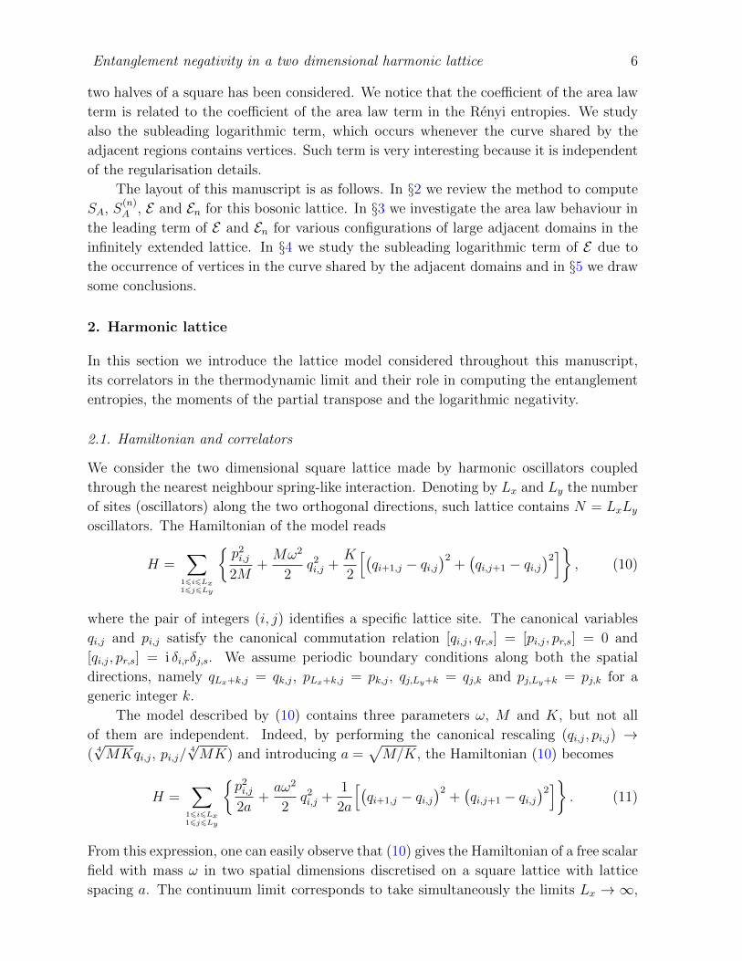
data for E of this configuration of adjacent domains are plotted in Fig. 1.
In the left panel we show the ratio E/`y as function of `x when `y is kept fixed. For any
given `y, such ratio reaches a constant value when `x is sufficiently large. This confirms
the intuition that the main contribution to a quantity characterising the entanglement
between two adjacent regions A1 and A2 should come from the degrees of freedom localized
along their shared boundary, namely the curve ∂A1 ∩ ∂A2. In the right panel of Fig. 1,
the logarithmic negativity of the same configuration is plotted as function of `y for fixed
values of `x. If `x is sufficiently large, a neat linear growth can be observed. The fact that
Entanglement negativity in a two dimensional harmonic lattice 10
Figure 1. Area law behaviour for the logarithmic negativity E between two equal
rectangles, whose edges have lengths `x and `y, which are adjacent along the vertical edge
(inset of the left panel). Left: For fixed values of `y, the ratio E/`y reaches a constant
value as `x increases. Right: For fixed and large enough values of `x, the logarithmic
negativity grows linearly as `y increases (the dashed line is obtained by fitting all the
data corresponding to `x = 11).
the asymptotic value of E/`y depends on `y in the left panel of Fig. 1 is mainly due to the
subleading corner contributions, which will be largely discussed in §4.
These results tell us that, given two equal and large enough adjacent regions A1 and
A2, at leading order the logarithmic negativity E between them increases like the length
of the curve ∂A1 ∩ ∂A2 shared by their boundaries as their size increases. Such length
will be denoted by Pshared ≡ length(∂A1 ∩ ∂A2) throughout this manuscript. Thus, the
logarithmic negativity between large adjacent domains satisfies an area law in terms of
the region shared by their boundaries. This observation has been recently done for this
model also by Eisler and Zimboras [34], who have considered the logarithmic negativity
between the two halves of a square as the length of its edge increases.
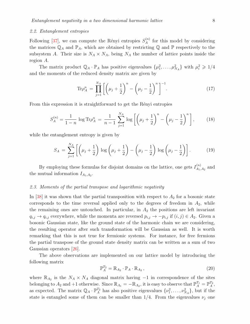
In order to improve our analysis of the area law behaviour for the logarithmic
negativity between adjacent regions A1 and A2, let us consider the six configurations
of adjacent domains on the lattice shown in Fig. 2, where the sites belonging to A1 and
A2 are highlighted by blue dots and red circles. In these examples the curve ∂A1 ∩ ∂A2
is not given by a simple line segment. The domains identified by the red circles in Fig. 2
are convex, while the ones corresponding to the blue dots are not.
It is well known that the curve separating adjacent domains on the lattice is not
unique. For these configurations we have chosen the dashed lines, which are the lines
whose length has been used to get the perimeter. The three configurations in the top
panels of Fig. 2 are natural to define on the square lattice because their edges are parallel
to the orthogonal vectors generating the lattice. Instead, the three configurations in
the bottom panels of Fig. 2 are made by adjacent domains where the line ∂A1 ∩ ∂A2
either is curved or it contains a line segment which is oblique with respect to the vectors
Entanglement negativity in a two dimensional harmonic lattice 11
Figure 2. Configurations of adjacent domains on the lattice, identified by red circles
and blue dots, which have been employed to study the area law behaviour (see §3 and
Figs. 3 and 4) and the corner contributions for explementary angles (see §4 and Fig. 5).
generating the lattice. Notice that a disk of given radius on the lattice could include a
different number of sites depending on whether the centre of the disk is located on a lattice
site or within a plaquette. Such ambiguity does not affect the leading order behaviour
of the quantities that we are considering, but it could be relevant for subleading terms
[14, 39].
Also for the logarithmic negativity of the adjacent domains shown in Fig. 2 we have
observed the same qualitative behaviour described in the left panel of Fig. 1 for the equal
adjacent rectangles: by keeping fixed the region corresponding to the red circles while the
sizes of the region characterised by the blue dots increase, E saturates to a constant value.
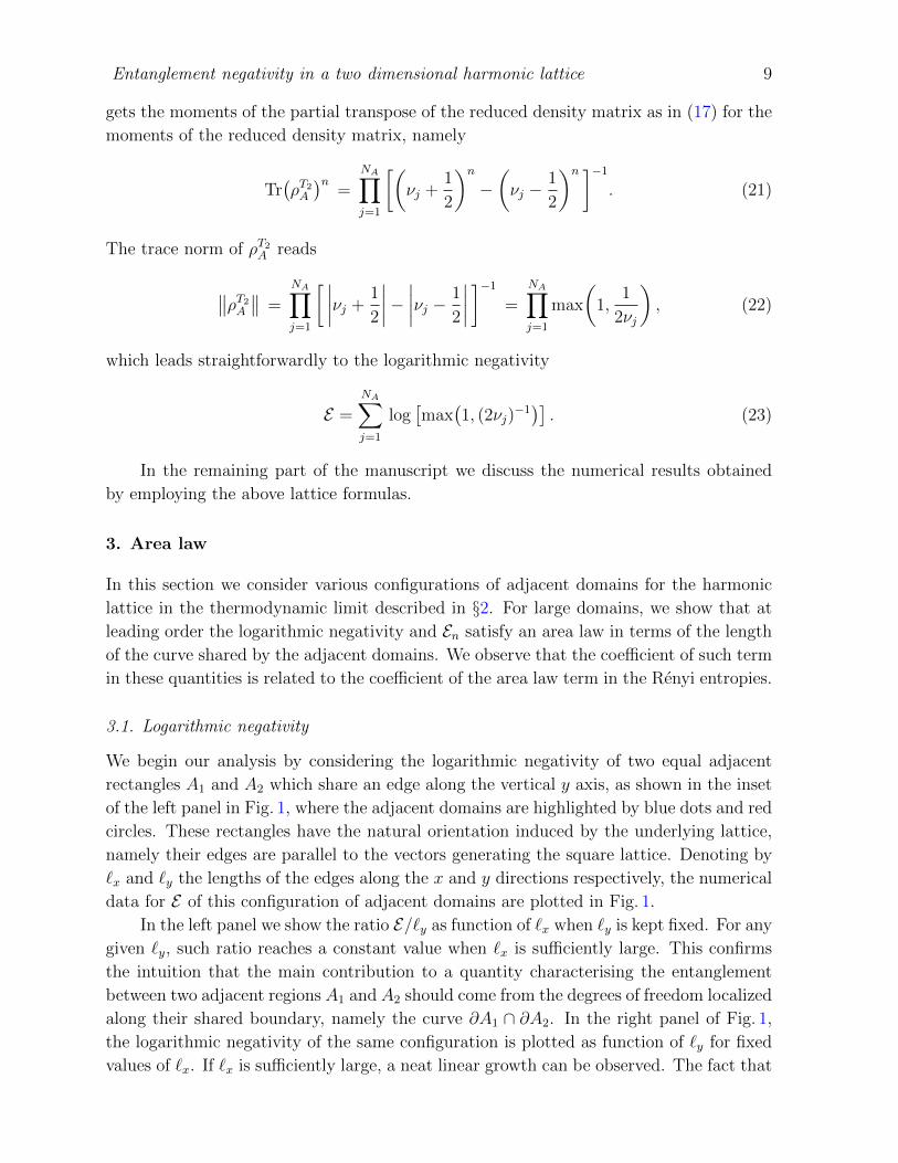
In Fig. 3 we show some quantitative results for the logarithmic negativity of the
configurations in Fig. 2. In particular, let us consider the configuration in the top left
panel, which is characterised by the lengths `in < `out of the edges of the internal square
and of the whole subregion A1 ∪ A2 respectively. In the left panel of Fig. 3 we show
E/`out as function of the ratio `in/`out < 1 when `out is kept fixed and the internal square
increases. For large enough `out, the area law behaviour in terms of `in is observed. It is
worth remarking that E → 0 when `in/`out → 1. This is expected because in this limit the
internal convex domain becomes the whole A. For any fixed and large enough value of `outthere is a critical size of the internal square after which the logarithmic negativity deviates
from the linear growth predicted by the area law. The numerical data tell us that such
critical value of `in increases by increasing `out. This suggests that in the continuum limit,
Entanglement negativity in a two dimensional harmonic lattice 12
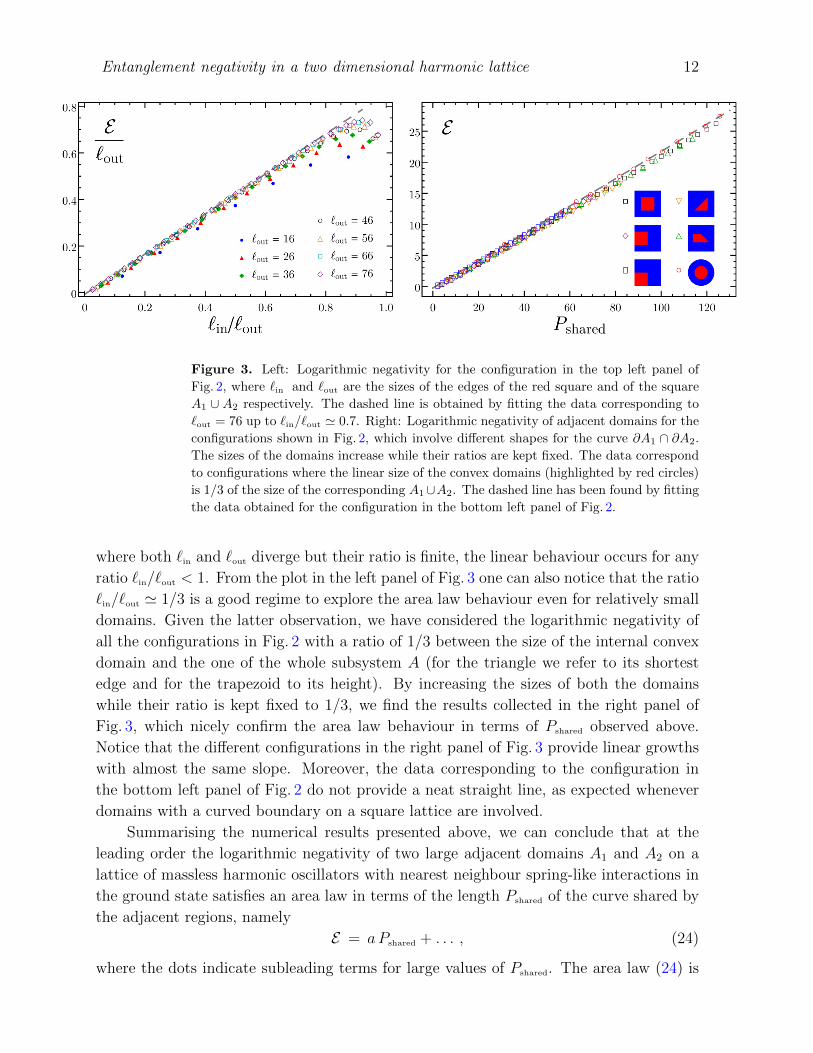
Figure 3. Left: Logarithmic negativity for the configuration in the top left panel of
Fig. 2, where `in and `out are the sizes of the edges of the red square and of the square
A1 ∪ A2 respectively. The dashed line is obtained by fitting the data corresponding to
`out = 76 up to `in/`out ' 0.7. Right: Logarithmic negativity of adjacent domains for the
configurations shown in Fig. 2, which involve different shapes for the curve ∂A1 ∩ ∂A2.
The sizes of the domains increase while their ratios are kept fixed. The data correspond
to configurations where the linear size of the convex domains (highlighted by red circles)
is 1/3 of the size of the corresponding A1∪A2. The dashed line has been found by fitting
the data obtained for the configuration in the bottom left panel of Fig. 2.
where both `in and `out diverge but their ratio is finite, the linear behaviour occurs for any
ratio `in/`out < 1. From the plot in the left panel of Fig. 3 one can also notice that the ratio
`in/`out ' 1/3 is a good regime to explore the area law behaviour even for relatively small
domains. Given the latter observation, we have considered the logarithmic negativity of
all the configurations in Fig. 2 with a ratio of 1/3 between the size of the internal convex
domain and the one of the whole subsystem A (for the triangle we refer to its shortest
edge and for the trapezoid to its height). By increasing the sizes of both the domains
while their ratio is kept fixed to 1/3, we find the results collected in the right panel of
Fig. 3, which nicely confirm the area law behaviour in terms of Pshared observed above.
Notice that the different configurations in the right panel of Fig. 3 provide linear growths
with almost the same slope. Moreover, the data corresponding to the configuration in
the bottom left panel of Fig. 2 do not provide a neat straight line, as expected whenever
domains with a curved boundary on a square lattice are involved.
Summarising the numerical results presented above, we can conclude that at the
leading order the logarithmic negativity of two large adjacent domains A1 and A2 on a
lattice of massless harmonic oscillators with nearest neighbour spring-like interactions in
the ground state satisfies an area law in terms of the length Pshared of the curve shared by
the adjacent regions, namely
E = aPshared + . . . , (24)
where the dots indicate subleading terms for large values of Pshared. The area law (24) is
Entanglement negativity in a two dimensional harmonic lattice 13
consistent with the fact that E measures the bipartite entanglement between A1 and A2
for the mixed state characterised by the reduced density matrix ρA1∪A2 . The coefficient a
in (24) is non universal, i.e. it depends on the ultraviolet details.
Given the two adjacent regions A1 and A2 considered above, another very interesting
quantity to study is their mutual information IA1,A2 , which has been defined in (3). Since
the area law of the entanglement entropy for large domains tells us that SA = a PA + . . . ,
it is straightforward to find that IA1,A2 of adjacent domains satisfies an area law in terms
of Pshared. In particular, we have that
IA1,A2 = 2a Pshared + . . . , (25)
where, as above, the dots stand for subleading terms.
3.2. Moments of the partial transpose
The moments Tr(ρT2A )n of the partial transpose for integer values of n are interesting
quantities to study because they provide the logarithmic negativity through the replica
limit (6) [22, 23].
Given the configurations of adjacent domains described in §3.1, instead of considering
the n-th moment of the partial transpose, we find it more interesting the ratio En defined
in (8), which also provides the logarithmic negativity through the replica limit (9) because
of the normalisation condition TrρA = 1. In our model, the main reason to consider Eninstead of log Tr(ρT2)n occurring in (6) is that, by repeating the analysis described in §3.1,
we find that, at leading order for large adjacent domains, En follows an area law in terms
of the length of the curve shared by the adjacent domains, i.e.
En = an Pshared + . . . , (26)
where the non universal coefficient an depends on the integer n and the dots denote
subleading terms. We recall that the Renyi entropies of our model satisfy the area law
S(n)A = an PA + . . . , where the coefficient an is non universal as well and limn→1 an = a.
From (26) and the area law of the Renyi entropies it is straightforward to find the
leading term of the logarithm of the moments of the partial transpose, which is given by
log Tr(ρT2A)n
= an Pshared + (1− n)an PA + . . . . (27)
Thus, the quantities log Tr(ρT2A )n contain an area law contribution also from the boundary
of A = A1 ∪ A2. Since limne→1(ne − 1)ane = 0, such term cancels in the replica limit
(6). A similar cancellation occurs also for adjacent intervals in 1 + 1 dimensional CFTs.
Indeed, considering the divergent terms for ε→ 0, in En only the ones giving a non trivial
contribution after the replica limit survive, while log Tr(ρT2)n contains also other terms
[23], which vanish in the replica limit (6). The quantity En for adjacent intervals in 1 + 1
dimensional CFTs has been studied in [25, 30] and for free fermions on a two dimensional
lattice in [34].
Entanglement negativity in a two dimensional harmonic lattice 14
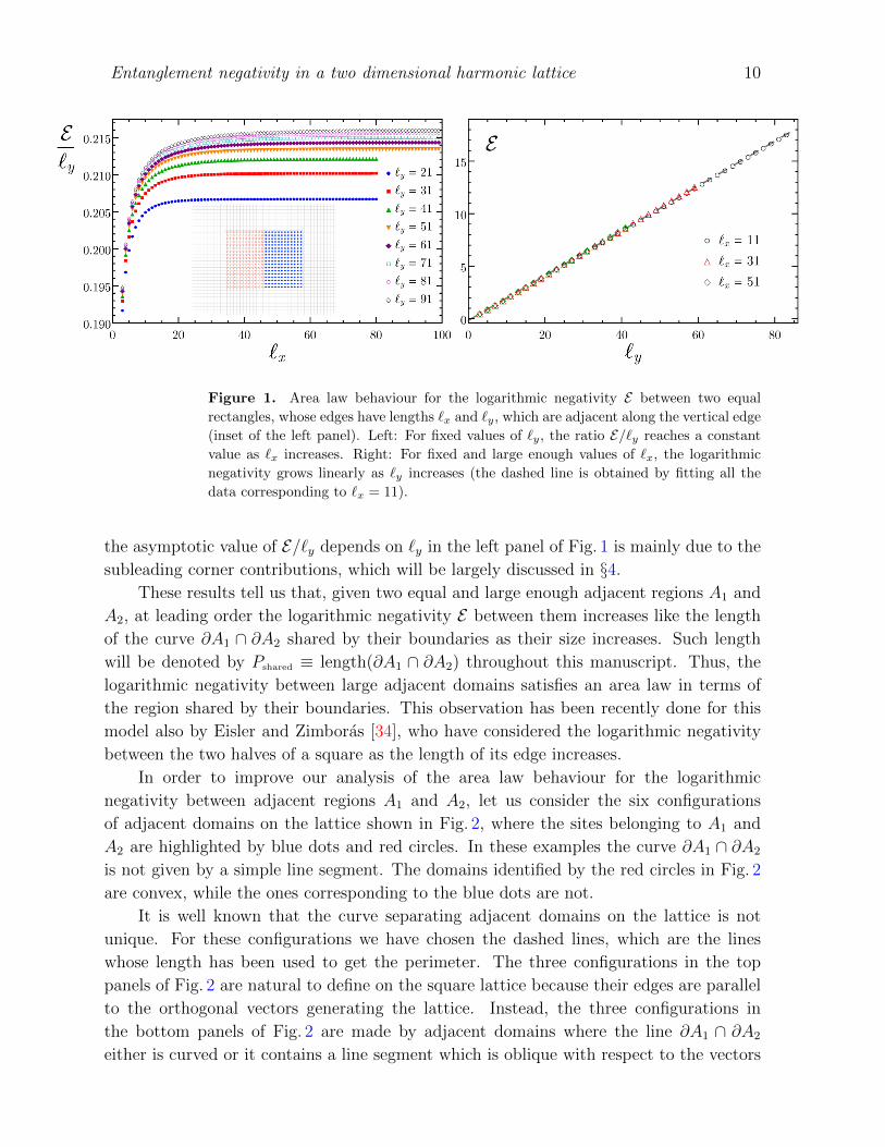
Figure 4. Left: The coefficient of the area law term in the Renyi entropies S(n)A as
function of n for domains with different shapes. centre The centres of the disks have
been chosen both on the lattice site and in the centre of a plaquette. Here the edges
of the square configuration are parallel to the vectors generating the lattice, while the
rhombus configuration corresponds to the previous square configuration rotated by π/4
with respect to its centre. Right: Numerical check of (29) and (30) for the configuration
in the bottom left panel of Fig. 2 with Rin/Rout = 1/3. Inset: The coefficient (1− n)anas function of n for disks (the data are taken from the left panel with the same colour
code). The black curve corresponds to the best fit of the numerical data through the
function f(n) = c−2/n2 + c−1/n + c0 + c1n, constrained by the condition f(1) = 0. In
the main plot the red curve is f(n) obtained in the inset and the green one is 2f(n/2).
In the left panel of Fig. 4 we show an as function of n for disks and squares on the
infinite lattice. The centres of the disks have been chosen either on a lattice site (like in
the bottom left panel of Fig. 2) or in the central point of a plaquette. As for the squares,
we have considered both the ones whose edges are parallel to the vectors generating the
lattice and the ones obtained by rotating of π/4 the previous ones (denoted as rhombi
in the plot). In this plot we have 150 6 Pshared 6 200, depending on the configuration.
A slight dependence of an on the shape can be observed from our data points. The
asymptotic an ∼ 1/n2 as n → 0 [40] is consistent with our numerical results. For the
Ising model a numerical analysis for an as n → 0 has been done in [41]. The numerical
data in the left panel of Fig. 4 have been found by employing a fitting function which
includes also a logarithmic term, as it will be discussed in detail in §4, but such term does
not change the coefficient of the leading area law term in a significant way.
It is worth considering the quantity I(n)A1,A2
= S(n)A1
+S(n)A2−S(n)
A1∪A2for the configurations
of adjacent domains described in §3.1. Given the area law behaviour of S(n)A , it is easy to
observe that I(n)A1,A2
displays an area law behaviour in terms of Pshared, namely
I(n)A1,A2
= 2an Pshared + . . . , (28)
Once the configuration of adjacent domains A1 and A2 has been chosen, we find it
interesting to compare the non universal coefficients an and an occurring in the area law
terms of (26) and (28) respectively.
Entanglement negativity in a two dimensional harmonic lattice 15
It is reasonable to expect that the area law term for En comes from effects localised
in the neighbourhood of the curve ∂A1 ∩ ∂A2. Thus, considering e.g. the configurations
in Fig. 2 where the domain identified by the red circles is entirely surrounded by the one
characterised by the blue dots (i.e. the configurations in the top left, bottom middle and
bottom right panels), such term should be independent of the size of the domain identified
by the blue dots. In the limit where this domain becomes the whole region complementary
to the one identified by the red circles, one gets the bipartition of the ground state. These
considerations suggest us that an in (26) is the same one occurring for a bipartition of
the ground state, when the identity (7) can be applied. This implies that the following
relation should hold
an =
{ (1− no
)ano odd n = no ,
2(1− ne/2
)ane/2 even n = ne .
(29)
Notice that a2 = 0, as expected. By employing the relation (29) and the replica limit
(9), it is straightforward to find that the coefficient of the area law term in the logarithmic
negativity in (24) is equal to the coefficient of the area law term in the Renyi entropy of
order 1/2, namely
a = a1/2 . (30)
In the right panel of Fig. 4 we show a numerical check of the relations (29) and (30)
for the configuration in the bottom left panel of Fig. 2. In particular, the coincidence of
the data points corresponding to n = 1/2 provides a check of (30). The solid curve in the
inset is obtained by fitting the data with the function f(n) = c−2/n2 + c−1/n+ c0 + c1n,
where the parameters are constrained by the requirement that f(1) = 0. Thus, such fit
has three independent parameters. As for the solid curves in the main plot, the red one
is f(n), namely the black curve found in the inset, while the green one is 2f(n/2).
This analysis has been performed also for other configurations as further checks of
(29) and (30), finding the same qualitative behaviours.
4. Logarithmic term from the corner contributions
In this section we consider the subleading logarithmic term in E and En for adjacent
domains, which occurs whenever the shared curve ∂A1 ∩ ∂A2 contains some vertices,
where its endpoints are included among them. For vertices corresponding to explementary
angles, we provide some numerical evidence that the corner function of E is given by the
corner function of the Renyi entropy of order 1/2.
4.1. Entanglement entropies
Let us consider the entanglement entropy SA of a connected domain A whose boundary
contains some vertices (see Figs. 2, 6 and 8 for examples). For large size of A, the leading
term gives the area law behaviour. The occurrence of vertices in ∂A provides a subleading
Entanglement negativity in a two dimensional harmonic lattice 16
logarithmic term which is characterised by a corner function b(θ) as follows [12, 13, 14]
SA = a PA −( ∑
verticesof ∂A
b(θi)
)logPA + . . . 0 < θi 6 π , (31)
where θi is the opening angle in A corresponding to the i-th vertex of ∂A and the dots
denote subleading terms.
Since the logarithmic term is due to the corners, we have that b(π) = 0. From the
general property that SA = SB for pure states and a bipartite Hilbert spaceH = HA⊗HB,
we have that b(θ) = b(2π−θ), which tells us that b(θ) is defined for 0 < θ 6 π. The model
dependent corner function b(θ) is universal, i.e. independent of the ultraviolet details of
the regularisation. In the continuum limit, which is described by a 2+1 dimensional CFT,
the corner function b(θ) contains important information about the model. For instance,
recently it has been found that the constant σ entering in the asymptotic behaviour
b(θ) = σ(π−θ)2+. . . as θ → π at the leading order is related to the constant characterising
the correlator 〈Tµν(x)Tαβ(y)〉 of the underlying CFT [16]. The corner function b(θ) for the
massless scalar has been studied by Casini and Huerta [12]. In the context of holography,
by employing the prescription of [18] for SA, the corner function b(θ) has been studied
e.g. in [19].
We find it worth considering the mutual information (3) of two adjacent domains
A1 and A2 when their boundaries contain some vertices. For the sake of simplicity, we
focus on configurations such that either two or three curves meet at every vertex. Explicit
examples are shown in Figs. 2, 6 and 8, where the adjacent domains are identified by blue
dots and red circles. In the scaling limit, when their sizes increase while the ratios among
them are kept fixed, from (31) one finds that
IA1,A2 = 2a Pshared −( ∑
vertices of∂A1 ∩ ∂A2
[b(θ
(1)i ) + b(θ
(2)i )− b(θ(1∪2)i )
])log `+ . . . , (32)
where ` is a parameter characterising the common size of the adjacent regions, θ(k)i is the
angle in Ak and θ(1∪2)i the angle in A1 ∪A2 corresponding to the i-th vertex belonging to
∂A1 ∩ ∂A2. In the simplest case where such vertex is not an endpoint of ∂A1 ∩ ∂A2, it
provides a bipartition of the angle of 2π and the corresponding contribution to the sum
in (32) is 2b(θ(1)i ) = 2b(θ
(2)i ).
We find it instructive to consider explicitly the examples in Figs. 2 and 6. For the
configurations shown in the top left, middle and right panel of Fig. 2, the sum within
the parenthesis multiplying the logarithmic term in (32) is given by 8b(π/2), 8b(π/2) and
6b(π/2) respectively, while for the bottom middle and right panels of the same figure
it reads 4b(π/4) + 2b(π/2) and 2b(π/4) + 4b(π/2) + 2b(3π/4) respectively. As for the
configurations of Fig. 6, such coefficient is 4b(π/4)− 2b(π/2), 3b(π/4) + b(3π/4)− b(π/2)
and 4b(π/2) for the top left, middle and right panels respectively, while it is given by
3b(π/4) + b(3π/4) − 2b(π/2), 2b(π/2) and 2b(π/4) + 2b(3π/4) − 2b(π/2) for the bottom
left, middle and right panels respectively. It is not difficult to get the coefficient of the
Entanglement negativity in a two dimensional harmonic lattice 17
logarithmic term also for the configurations in Fig. 8. Let us point out that for the one in
the top left panel such coefficient is vanishing.
As for the Renyi entropies of domains with non smooth boundary, we have that
S(n)A = an PA −
( ∑verticesof ∂A
bn(θi)
)logPA + . . . , (33)
where the corner function bn(θ) depends on the order n and it provides b(θ) through the
replica limit, i.e. limn→1 bn(θi) = b(θi). For the model we are dealing with, the corner
function bn(θ) has been found in [12]. A formula similar to (32) can be written for I(n)A1,A2
,
by just replacing a with an and b(θ) with bn(θ).
4.2. Logarithmic negativity
Considering the scaling limit for the configurations of adjacent domains A1 and A2 in
Figs. 2, 6 and 8 where ∂A1 and ∂A2 contain vertices, the expansion of the logarithmic
negativity contains a subleading logarithmic term after the leading area law term. By
analogy with the case of the entanglement entropy, it is reasonable to expect that the
coefficient of the logarithmic term is obtained by summing the contributions of the vertices
occurring in ∂A1 and ∂A2. Extracting the coefficient of such subleading logarithmic term
from the lattice numerical data is a delicate task.
Let us first discuss the method employed to get the numerical values presented in
this section from the formulas discussed in §2. A first rough approach could consist
in fitting the numerical data by a linear term, a logarithmic term and a constant
one. Nevertheless, since the logarithmic contribution is tiny with respect to the linear
one, its estimation can be spoiled by the occurrence of subleading lattice effects. In
order to take them into account, we have inserted in our fitting analysis also some
standard power law corrections, i.e. we have fitted our data with a function of the form
c1`+ clog log(`) + c0 + c−1`−1 + · · ·+ c−kmax`
−kmax [12, 14], where ` is a characteristic length
of Pshared. In particular, considering the domains identified by red circles in Figs. 2, 6 and
8, in each configuration ` corresponds to the edge for squares, to the shortest edge for
the triangles, to the radius for the disks and to the height for the trapezoids. For each
data set, in the plots we show the results of various fits performed in different ranges of `,
where each range is specified by the starting value `start and by the ending value `end. We
fix some maximum exponent kmax and some `start by removing some initial points, which
are strongly affected by lattice effects and therefore would need more corrections. Then,
we plot the logarithmic coefficient obtained from different fits as a function of `end. The
parameters kmax, `start and the maximum value of `end are chosen in order to get a stable
result from the fits in the whole range of `end. The logarithmic coefficient is estimated as
the average of the fitted values within such range of `end. The error introduced through
this procedure is estimated by taking the maximum deviation of the data from the average
within this range of stability.
Entanglement negativity in a two dimensional harmonic lattice 18
An important benchmark employed to test our numerical analysis is the mutual
information of adjacent domains. In particular, we have considered the coefficient of the
logarithmic term in the mutual information for the configurations in the top left, bottom
middle and bottom right panels of Fig. 2, recovering the values of the corner function b(θ)
for θ ∈ {π/4, π/2, 3π/4} available in the literature [12, 14, 42].
Let us consider the occurrence of a subleading logarithmic term due to corners in the
logarithmic negativity of some configurations of adjacent domains. We first observe that
the angles of A1 and A2 contributing to the logarithmic term in E are such that at least
one of their sides belongs to ∂A1 ∩ ∂A2, namely only the angles whose vertices lie on the
curve ∂A1 ∩ ∂A2 provide a non trivial logarithmic contribution. Also the endpoints of
∂A1 ∩ ∂A2 have to be included among such vertices. This is expected from the guiding
principle that the logarithmic negativity measures the entanglement between A1 and A2.
A way to check numerically this observation is to consider e.g. the coefficients of
the logarithmic terms in E for the configurations in the top panels of Fig. 2. These
configurations contain only three possible different contributions corresponding to this
kind of vertices. Thus, one can easily solve the resulting linear system of three equations
finding that the contribution coming from the four vertices which do not belong to
∂A1 ∩ ∂A2 is much smaller than the other ones (by a factor of about 1/100). As further
check that only the vertices lying on ∂A1 ∩ ∂A2 (including its endpoints) contribute to
the logarithmic term of E , we have constructed another configuration of adjacent domains
as follows: starting from a configuration like the one in the top right panel of Fig. 2 with
`in/`out = 1/3 and dividing the domain corresponding to the blue dots along the diagonal
with negative slope of A1 ∩ A2, we have removed the upper triangle. In the resulting
configuration A1 ∪ A2 is a triangle and the subregion identified by the red circles is a
square. Comparing the coefficients of the logarithmic term for this configuration and the
one for the configuration in the top right panel of Fig. 2 with `in/`out = 1/3, we have found
the same number within numerical errors.
Thus, the logarithmic negativity of adjacent domains whose boundaries share a curve
containing some vertices, where its endpoints are counted among them, is given by
E = aPshared −( ∑
vertices of∂A1 ∩ ∂A2
b(θ(1)i , θ
(2)i )
)logPshared + . . . , (34)
being θ(k)i the angle corresponding to the i-th vertex of ∂A1∩∂A2 which belongs to Ak. In
(34) we have assumed that either two or three curves meet at every vertex of ∂A1 ∩ ∂A2,
i.e. every vertex corresponds either to a bipartition (θ(1)i + θ
(2)i = 2π) or to a tripartition
(θ(1)i + θ
(2)i < 2π) respectively of the angle of 2π. This assumption, which has been done
also in (32), is verified for all the configurations in Figs. 2, 6 and 8.
From our numerical analysis, we find that the above considerations apply also for the
quantity En defined in (8). Thus we have
En = an Pshared −( ∑
vertices of∂A1 ∩ ∂A2
bn(θ(1)i , θ
(2)i )
)logPshared + . . . , (35)
Entanglement negativity in a two dimensional harmonic lattice 19
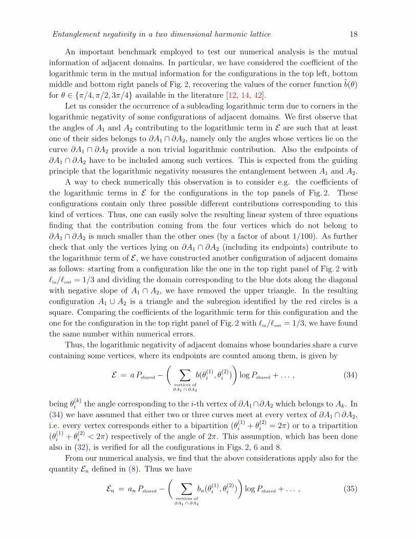
Figure 5. Stability analysis of the fitted values of the corner functions b(θ, 2π − θ)
and b1/2(θ) for θ ∈ {π/4, π/2, 3π/4}, as explained in §4.2. The configurations employed
here are shown in the top left, bottom middle and bottom right panels of Fig. 2. The
horizontal lines (with various dashing) correspond to the estimates obtained as explained
in §4.2. The numerical values are b(π/4, 7π/4) = 0.0977(3), b(π/2, 3π/2) = 0.029(1) and
b(3π/4, 5π/4) = 0.0060(5).
where the coefficient an has been already discussed in §3.2 and the corner function
bn(θ(1)i , θ
(2)i ) is related to the one occurring in the logarithmic term of (34) through the
replica limit (9), namely limne→1 bne(θ(1)i , θ
(2)i ) = b(θ
(1)i , θ
(2)i ).
Among the vertices belonging to the curve ∂A1 ∩ ∂A2 which contribute to the
logarithmic term in (34) and (35), let us consider first the ones corresponding to pairs of
explementary angles, i.e. the ones such that θ(1)i +θ
(2)i = 2π. This kind of vertices occurs in
all the panels of Fig. 2 except for the bottom left one (in particular, for the configurations
in the top left, bottom middle and bottom right panels only this kind of vertices occurs),
while it does not occur at all in the configurations of Fig. 6.
For these vertices we can make an observation similar to the one that leads to (29).
Indeed, because of the local nature of the function bn(θi, 2π−θi), it is reasonable to assume
that these vertices provide the same contribution given in the case of a bipartition of the
ground state, when (7) holds. This observation leads us to propose the following relation
between bn(θ, 2π − θ) and the corner function bn(θ) entering in the Renyi entropies
bn(θ, 2π − θ) =
{ (1− no
)bno(θ) odd n = no ,
2(1− ne/2
)bne/2(θ) even n = ne .
(36)
By employing the replica limit (9), the relation (36) allows to conclude that the corner
function in the logarithmic negativity for this kind of vertices is equal to the corner
Entanglement negativity in a two dimensional harmonic lattice 20
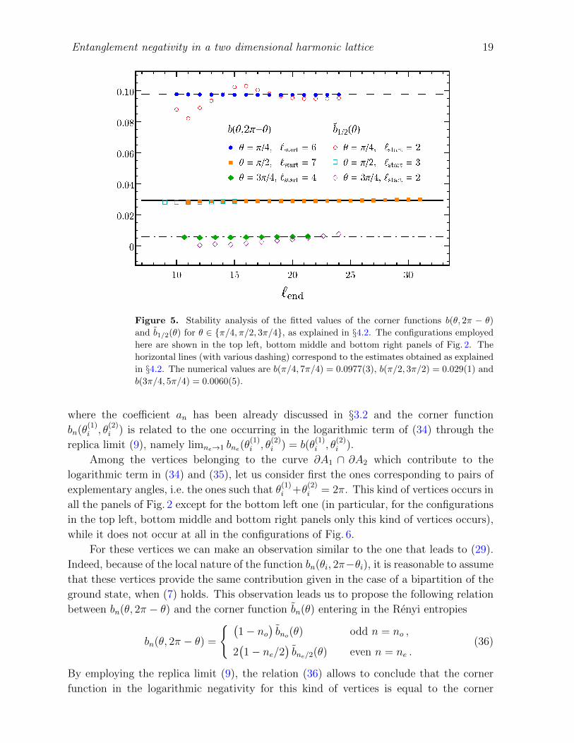
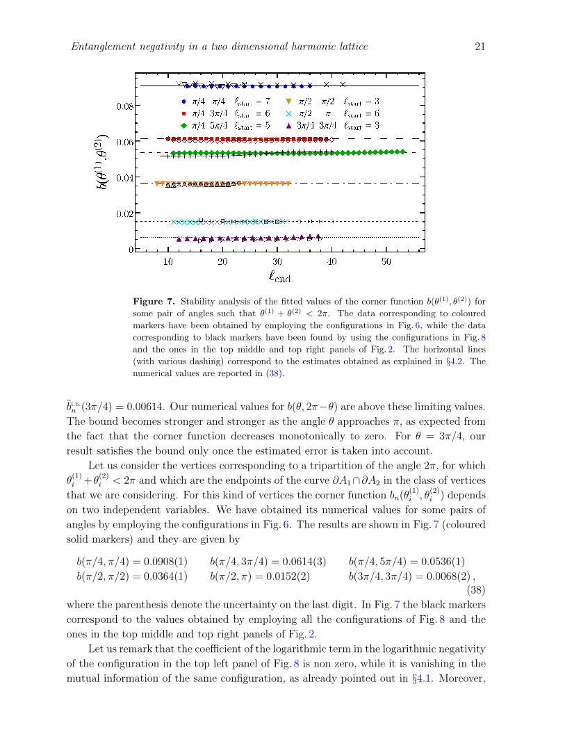
Figure 6. Configurations of adjacent domains on the lattice, identified by red circles and
blue dots, which have been employed to find b(θ(1), θ(2)) for some values of arguments
such that θ(1) + θ(2) < 2π (coloured markers in Fig. 7).
function in the Renyi entropy of order 1/2, namely
b(θ, 2π − θ) = b1/2(θ) . (37)
Numerical checks of the relation (37) for some values of θ are shown in Fig. 5. The values
of b(θ, 2π − θ) and b1/2(θ) for θ ∈ {π/4, π/2, 3π/4} have been found by evaluating E and
I(1/2)A1,A2
for the configurations shown in the top middle, bottom middle and bottom right
panels of Fig. 2, where the curve ∂A1 ∩ ∂A2 contains only the kind of vertices that we are
considering. The numerical values obtained for b(θ, 2π − θ) for the above opening angles