85
1/85 USE AND EVALUATION OF M-MACBETH Cristina Gómez, Jesús Ladevesa, Laura Prieto Raimon Redondo, Karina Gibert, Aïda Valls Juliol 2007 DEIM-RT-07-004

1/85
USE AND EVALUATION OF M-MACBETH
Cristina Gómez, Jesús Ladevesa, Laura Prieto Raimon Redondo, Karina Gibert, Aïda Valls
Juliol 2007
DEIM-RT-07-004
TABLE OF CONTENTS Chapter 1 – Introduction ......................................................................................................................1
1.1 What is MACBETH?.................................................................................................................1 1.2 About this document ..................................................................................................................1
Chapter 2 - Mathematical foundations.................................................................................................3 2.1 Types of preferential information ..............................................................................................4
2.1.1 Type 1 information..............................................................................................................4 2.1.2 Type 1+2 information .........................................................................................................4
2.2 Numerical representation of the preferential information..........................................................5 2.2.1 Type 1 scale ........................................................................................................................5 2.2.2- Type 1+2 scale...................................................................................................................5
2.3- Consistency and inconsistency .................................................................................................5 2.4- Consistency test for preferential information ...........................................................................6
2.4.1- Testing procedures.............................................................................................................6 2.4.2- Pre-test of the preferential information..............................................................................6 2.4.3- Consistency test for type 1 information.............................................................................7 2.4.3.1- Consistency test for incomplete (? ≠φ ) type 1 information ...........................................7 2.4.3.2- Consistency test for complete (? =φ ) type 1 information ..............................................7 2.4.4- Consistency test for type 1+2 information ........................................................................7
2.5- The MACBETH scale...............................................................................................................8 2.5.1- Definition of the MACBETH scale ...................................................................................8 2.5.2- Discussing the uniqueness of the basic MACBETH scale ................................................8 2.5.3- Presentation of the MACBETH scale..............................................................................10
2.6- Discussion about a scale .........................................................................................................10 Chapter 3 - Getting Started ................................................................................................................13
3.1 First example: buying a car......................................................................................................13 3.2 Creating a M-MACBETH file .................................................................................................13
Chapter 4 - Structuring a M-MACBETH Model ...............................................................................15 4.1 Fundamentals of structuring.....................................................................................................15 4.2 Defining the options.................................................................................................................16
4.2.1 Entering options into the model .....................................................................................16 4.3 Building the value tree and defining criteria............................................................................17
4.3.1 Types of nodes and bases for comparison ........................................................................17 4.3.2 Entering non-criterion nodes..........................................................................................17 4.3.3 Entering criterion nodes with a direct basis for comparison.............................................18 4.3.4 Entering criterion nodes with an indirect basis for comparison........................................19
4.4 Entering option’s performances into the model.......................................................................23 Chapter 5 - Scoring ............................................................................................................................25
5.1 Ranking within a criterion........................................................................................................25 5.2 Qualitatively judging differences of attractiveness within a criterion .....................................26 5.3 Sorting out inconsistencies ......................................................................................................26 5.4 Quantifying attractiveness within a criterion ...........................................................................28
5.4.1 Quantifying attractiveness from the comparison of options .........................................28 5.4.2 Filling up the criterions tables...........................................................................................29
Chapter 6 - Weighting........................................................................................................................31 6.1 Weighting references ...............................................................................................................31 6.2 Ranking the weights.................................................................................................................32 6.3 Qualitatively judging differences of overall attractiveness......................................................33 6.4 Quantifying the weights ...........................................................................................................33

Chapter 7 - Analysing the Model’s Results .......................................................................................35 7.1 Overall scores...........................................................................................................................35 7.2 Table of rankings .....................................................................................................................35 7.3 Overall thermometer ................................................................................................................36 7.4 Option’s profiles ......................................................................................................................37 7.5 Differences profiles..................................................................................................................38 7.6 XY mapping.............................................................................................................................39
7.6.1 Comparing scores in two criteria or groups of criteria ..................................................39 7.6.2 “Cost-Benefit” analysis.....................................................................................................40
Chapter 8 - Sensitivity and Robustness Analyses..............................................................................43 8.1 Sensitivity Analyses.................................................................................................................43
8.1.1 Sensitivity Analysis on a criterion weight ........................................................................43 8.1.2 Software interactivity....................................................................................................44
8.2 Robustness Analysis ................................................................................................................44 Chapter 9 – Analysis of countries using M-Macbeth ........................................................................47
9.1 Data Set Characteristics ...........................................................................................................47 9.2 Data Introduction .....................................................................................................................49 9.3 Results......................................................................................................................................55
9.3.1 Overall Scores ...................................................................................................................55 9.3.2 Overall Thermometer........................................................................................................57 9.3.3 Option’s Profiles ...............................................................................................................58 9.3.4 Differences Profiles ..........................................................................................................64 9.3.5 XY Mapping .....................................................................................................................68 9.3.6 Robustness Analysis .........................................................................................................70
9.4 Modifications ...........................................................................................................................72 9.5 Global Comparison ..................................................................................................................79
Chapter 10 - Conclusions...................................................................................................................81 References..........................................................................................................................................82

1
Chapter 1 – Introduction
1.1 What is MACBETH?
MACBETH stands for Measuring Attractiveness through a Category Based Evaluation Technique. This decision making method permits the evaluation of options against multiple criteria. The key distinction between MACBETH and other Multiple Criteria Decision Analysis (MCDA) methods is that it needs only qualitative judgements about the difference of attractiveness between two elements at a time, in order to generate numerical scores for the options in each criterion and to weight the criteria. The seven MACBETH semantic categories are: no, very weak, weak, moderate, strong, very strong, and extreme difference of attractiveness.
As the judgements expressed by the evaluator are entered in the M-MACBETH software (www.m-macbeth.com), their consistency is automatically verified and suggestions are offered to resolve inconsistencies if they arise. The MACBETH decision aid process then evolves into the construction of a quantitative evaluation model. Using the functionalities offered by the software, a value scale for each criterion and weights for the criteria are constructed from the evaluator’s semantic judgements. The value scores of the options are subsequently aggregated additively to calculate the overall value scores that reflect their attractiveness taking all the criteria into consideration.
Extensive analysis of the sensitivity and robustness of the model’s results will then provide a deeper understanding of the problem, contributing to attain a requisite evaluation model: a sound basis to prioritise and select options in individual or group decision-making contexts. M-MACBETH can be downloaded from: http://www.m-macbeth.com
Users have to register if they want to download a demo version of the program (it just uses to academic purposes). To install it, the user must execute the downloaded file. Inside the program (in the “Help” option), there is a very complete M-MACBETH Users Guide. For this reason, this document doesn’t give details about M-MACBETH uses, but the results of applying this software to our data.
A problem was detected during the installation of this software. It was that the user can not choose the path where the data model will be installed (default option where user has his document files).
This demo version limits the number of criteria to a maximum of 4.
1.2 About this document
This document pretends to explain the most important tools of the M-MACBETH software, which implements the MACBETH methodology. It is not intended to exhaustively introduce all of M-MACBETH’s capabilities. In chapter 2 we review the mathematical basis of this multicriteria decision making method. In the chapters 3 to 8 we proceed to introduce each step of the model building process with an illustrative example allowing you to build your own MACBETH model. Then, in chapter 9 we will analyse a second case study about Countries. In this case study different modifications to the data set are done and the differences in the results are highlighted.
It is worth to mention that the analysis done follow the key stages in a multicriteria decision aiding process, which are usually grouped into three main phases:

2
Structuring: Criteria: Structuring the values of concern and identifying the criteria. Options: Defining the options to be evaluated as well as their performances.
Evaluating: Scoring: Evaluating each option’s attractiveness with respect to each criterion. Weighting: Weighting the criteria.
Recommending: Analysing Results: Analysing options’ overall attractiveness and exploring the model results. Sensitivity Analyses: Analysing the sensitivity and robustness of the model’s results in light of several types of data uncertainty.
The order in which these activities are performed in practice, as well as which of them are necessary, is dependant upon the specifics of the decision context.

3
Chapter 2 - Mathematical foundations
Let X (with #X = n ≥ 2) be a finite set of elements (alternatives, choice options, courses of action) that an individual or a group, J, wants to compare in terms of their relative attractiveness (desirability, value). Ordinal value scales (defined on X) are quantitative representations of preferences that reflect, numerically, the order of attractiveness of the elements of X for J. The construction of an ordinal value scale is a straightforward process, provided that J is able to rank the elements of X by order of attractiveness – either directly or through pairwise comparisons of the elements to determine their relative attractiveness. Once the ranking is defined, one needs only to assign a real number v(x) to each element x of X, in such a way that: 1- v(x) = v(y) if and only if J judges the elements x and y to be equally attractive. 2- v(x) > v(y) if and only if J judges x to be more attractive than y. A value difference scale (defined on X) is a quantitative representation of preferences that is used to reflect, not only the order of attractiveness of the elements of X for J, but also the differences of their relative attractiveness, or in other words, the strength of J ’s preferences for one element over another. Using MACBETH, J is asked to provide preferential information about two elements of X at a time, firstly by giving a judgement as to their relative attractiveness (ordinal judgement) and secondly, if the two elements are not deemed to be equally attractive, by expressing a qualitative judgement about the difference of attractiveness between the most attractive of the two elements and the other. Moreover, to ease the judgemental process, six semantic categories of difference of attractiveness, “very weak”, “weak”, “moderate”, “strong”, “very strong” or “extreme”, or a succession of these (in case hesitation or disagreement arises) are offered to J as possible answers. By pairwise comparing the elements of X a matrix of qualitative judgements is filled in, with either only a few pairs of elements, or with all of them (in which case n · (n - 1)/ 2 comparisons would be made by J). This section will use the following notation: - J is an evaluator, either an individual or group. - X (with #X = n ≥ 2) is a finite set of elements (alternatives, choice options, courses of action) that J wants to compare in terms of their relative attractiveness (desirability, value). - Δatt(x,y) is the “difference of attractiveness between x and y for J ”, where x and y are elements of X such that x is more attractive than y for J. - φ is an empty set. - R is the set of real numbers. - *
+R = {x∈R | x ≥ 1}. - N is the set of non-negative integer numbers. - Ns, t = {s, s+1, …, t} = {x ∈ N | s ≤ x ≤ t} where s, t ∈ N, and s < t.
4
2.1 Types of preferential information
2.1.1 Type 1 information Let x and y be two different elements of X. Type 1 information refers to preferential information obtained from J by means of the following procedure: - A first question is asked of J: Is one of the two elements more attractive than the other? - J ’s response can be: “Yes”, “No”, or “I don’t know”. - If the response is “Yes”, a second question is asked: Which of the two elements is the most attractive? The responses to this procedure for several pairs of elements of X enable the construction of three binary relations on X: - P = {(x,y) ∈ X×X : x is more attractive than y} - I = {(x,y) ∈ X×X : x is not more attractive than y and y is not more attractive than x, or x = y} - ? = {(x,y) ∈ X×X : x and y are not comparable in terms of their attractiveness} Type 1 information about X is a structure {P, I, ?} where P, I and ? are disjoint relations on X.
2.1.2 Type 1+2 information Suppose that type 1 information {P, I, ?} about X is available. Now we have this procedure: - The following question is asked, for all (x,y) ∈ P: How do you judge the difference of attractiveness between x and y? - J ’s response would be provided in the form “ds” (where d1, d2,…,dQ (Q ∈ N \ {0,1}) are semantic categories of difference of attractiveness defined so that if i < j, the difference of attractiveness “di” is weaker than the difference of attractiveness “dj”) or in the more general form (possibility of hesitation) “ds to dt”, with s ≤ t (the response “I don’t know” is assimilated to the response “d1 to dQ”). When Q = 6 and d1 = very weak, d2 = weak, d3 = moderate, d4 = strong, d5 = very strong and d6 = extreme, this procedure is the mode of interaction used in the MACBETH approach and its M-MACBETH software. Type 1+2 information about X is a structure {P, I, ?, Pe} where {P, I, ?} is type 1 information about X and Pe is an asymmetric relation on P, the meaning of which is “(x,y) Pe (z,w) when Δatt(x,y) > Δatt(z,w)”.

5
2.2 Numerical representation of the preferential information
2.2.1 Type 1 scale Suppose that type 1 information {P, I, ?} about X is available. A type 1 scale on X relative to {P,I} is a function μ : X R satisfying: Condition 1: ∀ x, y ∈ X, [xPy⇒ μ(x) > μ(y)] and [xIy⇒ μ(x) = μ(y)]. Let Sc1(X, P, I) = {μ : X R | μ is a type 1 scale on X relative to {P, I}}. When X, P and I are well determined, Sc1(X, P, I) will be noted Sc1. When ? = φ and Sc1(X, P, I) ≠φ , each element of Sc1(X, P, I) is an ordinal scale on X.
2.2.2- Type 1+2 scale Suppose that type 1+2 information {P, I, ?, Pe} about X is available. A type 1+2 scale on X relative to {P, I, ?, Pe} is a function μ : X R satisfying condition 1 and: Condition 2: ∀ x, y, z, w ∈ X, [(x,y)Pe(z,w)⇒ μ(x) - μ(y) > μ(z) - μ(w)]. Let Sc1+2(X, P, I, Pe) = {μ : X R | μ is a type 1+2 scale on X relative to {P, I, Pe}}. When X, P, I and Pe are well determined, Sc1+2(X, P, I, Pe) will be noted Sc1+2.
2.3- Consistency and inconsistency Type 1 information {P, I, ?} about X is: - Consistent when Sc1(X, P, I) ≠φ . - Inconsistent when Sc1(X, P, I) =φ . Type 1+2 information {P, I, ?, Pe} about X is: - Consistent when Sc1+2(X, P, I, Pe) ≠φ . - Inconsistent when Sc1+2(X, P, I, Pe) =φ . When Sc1+2(X, P, I, Pe) =φ one can have: - Sc1(X, P, I) =φ : in this case, the message “no ranking” will appear in M-MACBETH; it occurs namely when J declares, in regards to elements x, y and z of X, that [xIy, yIz and xPz] or [xPy, yPz and zPx]. - Sc1(X, P, I) ≠φ : in this case, the message “inconsistent judgement” will appear in M-MACBETH. Although this is the only difference between the types of inconsistency introduced in M-MACBETH, it is interesting to mention, from a theoretical perspective, that one could further distinguish two sub-types of inconsistency when Sc1+2(X, P, I, Pe) =φ and Sc1(X, P, I) ≠φ :

6
- Sub-type a: inconsistency arises when there is a conflict between type 1 information and Pe that makes the simultaneous satisfaction of conditions 1 and 2 impossible. - Sub-type b: inconsistency arises when there is no conflict between type 1 information and Pe but at least one conflict exists inside Pe that makes satisfying condition 2 impossible.
2.4- Consistency test for preferential information
2.4.1- Testing procedures Suppose that X = {a1, a2, …, an}. During the interactive questioning process conducted with J, each time that a new judgement is obtained, the consistency of all the responses already provided is tested. This consistency test begins with a pre-test aimed at detecting the (potential) presence of cycles within the relation P and, if no such cycle exists, making a permutation of the elements of X in such a way that, in the matrix of judgements, all of the cells P or Cij will be located above the main diagonal. When there is no cycle in P, the consistency of type 1 information {P, I, ?} is tested as follows: - If ? ≠φ , a linear program named LP-test1 is used. - If ? =φ , rather than linear programming, a method named DIR-test1 is used, which has the advantage of being easily associated with a very simple visualization of an eventual ranking within the matrix of judgements. When {P, I, ?} is consistent, the consistency of type 1+2 information {P, I, ?, Pe} is tested with the help of a linear program named LPσ-test1+2.
2.4.2- Pre-test of the preferential information The algorithm PRETEST detects cycles within P and sorts the elements of X by making permutations of the elements. PRETEST: 1 s n; 2 among a1, a2, …, as find ai which is not preferred over any other:
if ai exists, go to 3; if not, return FALSE (Sc1 = φ ); finish.
3 permute ai and as; 4 s s – 1;
if s = 1, return TRUE; finish. if not, go to 2.
7
2.4.3- Consistency test for type 1 information Suppose that PRETEST detected no cycle within P and that the elements of X were renumbered as follows: ∀ i, j ∈ N1, n [i > j ⇒ ai(notP)aj].
2.4.3.1- Consistency test for incomplete (? ≠φ ) type 1 information
Consider the linear program LP-test1 with variables x1, x2, …, xn: min x1 subject to xi – xj ≥ dmin ∀ (ai,aj) ∈ P xi – xj = 0 ∀ (ai,aj) ∈ I with i ≠ j xi ≥ 0 ∀ i ∈ N1, n where dmin is a positive constant, and the variables x1, x2, …, xn represent the numbers μ(ai), μ(aj), …, μ(an) that should satisfy condition 1 so that μ is a type 1 scale. The objective function min x1 of LP-test1 is obviously arbitrary. It is trivial that Sc1 ≠ φ ⇔ LP-test1 is feasible.
2.4.3.2- Consistency test for complete (? =φ ) type 1 information
When ? =φ and the elements of X have been renumbered (after the application of PRETEST), another simple test (DIR-test1) allows one to verify if P∪ I is a complete preorder on X. Proposition: if [∀ i, j ∈ N1, n with i < j, (ai,aj) ∈ P∪ I ] then P∪ I is a complete preorder on X if and
only if ∀ i, j ∈ N1, n with i < j: ⎥⎥⎦
⎤
⎢⎢⎣
⎡
⎭⎬⎫
⎩⎨⎧
−≤≤∃≥∀≤∀
⇒+1,1:
,,
ss
tsji Paajsis
PaajtisPaa .
2.4.4- Consistency test for type 1+2 information To test the consistency of type 1+2 information, the efficient linear program LP-test1+2 is used, which includes “thresholds conditions” equivalent to conditions 1 and 2. LP-test1+2 is based on the following lemma: - Let μ : X R. μ satisfies conditions 1 and 2 if and only if there exist Q “thresholds” 0 < σ1 < σ2 < … < σ Q that satisfy this conditions:
-∀ (x,y) ∈ I, μ(x) = μ(y) -∀ i, j ∈ N1, Q with i ≤ j, ∀ (x,y) ∈ Cij, σi < μ(x) - μ(y) -∀ i, j ∈ N1, Q-1 with i ≤ j, ∀ (x,y) ∈ Cij, μ(x) - μ(y) < σj+1

8
Program LP-test1+2 has variables x1(= μ(a1)), …, xn(= μ(an)), σ1, …, σ Q: min x1 subject to xp – xr = 0 ∀ (ap,ar) ∈ I with p < r σj + dmin ≤ xp – xr ∀ i, j ∈ N1, Q with i ≤ j,∀ (ap,ar) ∈ Cij xp – xr ≤ σj+1 – dmin ∀ i, j ∈ N1, Q-1 with i ≤ j,∀ (ap,ar) ∈ Cij dmin ≤ σ1 σi-1 + dmin ≤ σi ∀ i ∈ N2, Q xi ≥ 0 ∀ i ∈ N1, n σi ≥ 0 ∀ i ∈ N1, Q Taking into account the previous lemma, it is trivial that Sc1+2 ≠ φ if and only if the linear program LP-test1+2 which is based on the previous conditions is feasible.
2.5- The MACBETH scale
2.5.1- Definition of the MACBETH scale Suppose that Sc1+2 ≠ φ and a1(P∪ I)a2…an-1(P∪ I)an. The linear program LP-MACBETH with variables x1, …, xn, σ1, …, σQ is therefore feasible:
min x1 subject to xp – xr = 0 ∀ (ap,ar) ∈ I with p < r σi + 1/2 ≤ xp – xr ∀ i, j ∈ N1, Q with i ≤ j,∀ (ap,ar) ∈ Cij xp – xr ≤ σj+1 – 1/2 ∀ i, j ∈ N1, Q-1 with i ≤ j,∀ (ap,ar) ∈ Cij σ1 = 1/2 σi-1 + 1 ≤ σi ∀ i ∈ N2, Q xi ≥ 0 ∀ i ∈ N1, n σi ≥ 0 ∀ i ∈ N1, Q Any function EchMac : X R such that ∀ i∈N1, n , EchMac(ai) = *
ix , where ( *1x ,…, *
nx ) is an optimal solution of LP-MACBETH, is called a basic MACBETH scale. ∀ a∈ *
+R ,∀ b∈R with (a,b) ≠ (1,0), a · EchMac + b is a transformed MACBETH scale.
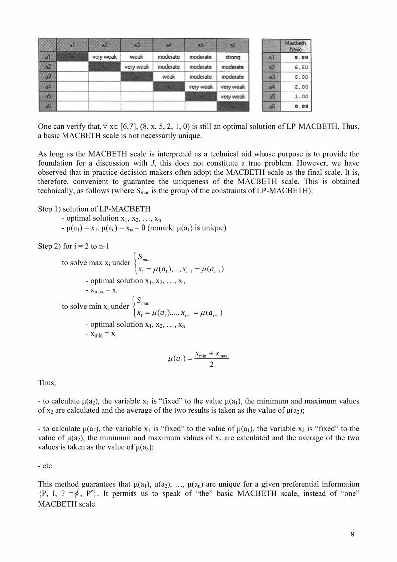
2.5.2- Discussing the uniqueness of the basic MACBETH scale Nothing guarantees that a LP-MACBETH optimal solution is unique. For example, consider the matrix of judgements and the basic MACBETH scale shown the figure:
9
One can verify that,∀ x∈[6,7], (8, x, 5, 2, 1, 0) is still an optimal solution of LP-MACBETH. Thus, a basic MACBETH scale is not necessarily unique. As long as the MACBETH scale is interpreted as a technical aid whose purpose is to provide the foundation for a discussion with J, this does not constitute a true problem. However, we have observed that in practice decision makers often adopt the MACBETH scale as the final scale. It is, therefore, convenient to guarantee the uniqueness of the MACBETH scale. This is obtained technically, as follows (where Smac is the group of the constraints of LP-MACBETH): Step 1) solution of LP-MACBETH
- optimal solution x1, x2, …, xn - μ(a1) = x1, μ(an) = xn = 0 (remark: μ(a1) is unique)
Step 2) for i = 2 to n-1
to solve max xi under ⎩⎨⎧
== −− )(),...,( 1111 ii
mac
axaxS
μμ
- optimal solution x1, x2, …, xn - xmax = xi
to solve min xi under ⎩⎨⎧
== −− )(),...,( 1111 ii
mac
axaxS
μμ
- optimal solution x1, x2, …, xn - xmin = xi
2)( maxmin xx
ai+
=μ
Thus, - to calculate μ(a2), the variable x1 is “fixed” to the value μ(a1), the minimum and maximum values of x2 are calculated and the average of the two results is taken as the value of μ(a2); - to calculate μ(a3), the variable x1 is “fixed” to the value of μ(a1), the variable x2 is “fixed” to the value of μ(a2), the minimum and maximum values of x3 are calculated and the average of the two values is taken as the value of μ(a3); - etc. This method guarantees that μ(a1), μ(a2), …, μ(an) are unique for a given preferential information {P, I, ? =φ , Pe}. It permits us to speak of “the” basic MACBETH scale, instead of “one” MACBETH scale.

10
2.5.3- Presentation of the MACBETH scale The MACBETH scale that corresponds to {P, I, ? =φ , Pe} consistent information is represented in two ways in M-MACBETH: a table and a “thermometer”. In this example, the transformed MACBETH scale represented in the thermometer was obtained by imposing the values of the elements d and c as 100 and 0 respectively:
Even though the values attributed to c and d are fixed, in general an infinite number of scales that satisfy conditions 1 and 2 exist. It is, thus, necessary to allow J to, should he or she want to, modify the values suggested.
2.6- Discussion about a scale Suppose that, in the previous example, J considers that the element a is badly positioned when compared to elements c and d, and therefore J wants to redefine the value of a. It is then interesting to show J the limits within which the value of a can vary without violating the preferential information provided by J. Let us suppose in this section that we have a type 1+2 information about X which is consistent and that ? = φ . Let μ0 be a particular scale of Sc1+2, L and H be two fixed elements of X with HPL (H more attractive than L) and a be an element of X (not indifferent to L and not indifferent to H) that J would like to have repositioned. Let - Sc(μ0, H, L) = {μ∈ Sc1+2 | μ(H) = μ0(H) and μ(L) = μ0(L)} (scales for which values associated with H and L have been fixed)

11
- Sc(μ0, â ) = {μ∈ Sc1+2 | ∀ y∈X with y not indifferent to a: μ(y) = μ0(y)} (scales for which the values of all of the elements of X except a and its eventual equals have been fixed). We call free interval associated to interval a:
We call dependent interval associated to interval a:
In the previous example, if one selects a, two intervals are presented to J (see next figure) which should be interpreted as follows:
The closed intervals (in the example [66.69, 99.98] and [72.74, 90.9]) that have been chosen to present to J are not the precise free and dependent intervals associated to a (which, by definition, are open); however, by taking a precision of 0.01 into account, they can be regarded as the “greatest” closed intervals included in the free and dependent intervals. M-MACBETH permits the movement of element a with the mouse but, obviously, only inside of the dependent interval associated to a.

12
If J wants to give element a a value that is outside of the dependent interval (but still inside the free interval), the software points out that the values of the other elements must be modified. If J confirms the new value of a, a new MACBETH scale is calculated, taking into account the additional constraint that fix the new value of a. The (“closed”) free interval is calculated by integer linear programming. The (“closed”) dependent interval could be also calculated in the same manner. However, M-MACBETH computes it by “direct” calculation formulas which make the determination of these intervals extremely fast.

13
Chapter 3 - Getting Started
3.1 First example: buying a car. John Doe is quite sure about the brand and model of the car he wants, the Peugeot 207. However, there is not only one version of this car model, so he decided to use M-MACBETH software to select the version of the car that most adequately fulfils his needs. The available models are 14, listed in Table 1. The different characteristics used to decide which car is better for his interests are the following: “Fuel consumption”, “Horsepower”, “Engine type” and “Accessory pack”.
Brand & Model Version Price PEUGEOT 207 207 1.4i 75 Urban 3P 12.268,77 € PEUGEOT 207 207 1.4i 75 X-Line 3P 13.190,00 € PEUGEOT 207 207 1.4i 16V 90 X-Line 3P 13.690,00 € PEUGEOT 207 207 1.4 HDi 70 Urban 3P 13.770,00 € PEUGEOT 207 207 1.4 HDi 70 X-Line 3P 14.690,00 € PEUGEOT 207 207 1.4i 16V 90 XS 3P 15.190,00 € PEUGEOT 207 207 1.6 HDi 90 X-Line 3P 15.490,01 € PEUGEOT 207 207 1.6 VTi 16V 120 XS 3P 15.890,00 € PEUGEOT 207 207 1.6 VTi 120 XS Pack 3P 16.740,00 € PEUGEOT 207 207 1.6 HDi 90 XS 3P 16.990,00 € PEUGEOT 207 207 1.6 HDi 90 XS Pack 3P 17.840,01 € PEUGEOT 207 207 1.6 HDi 110 XS Pack 3P 18.820,00 € PEUGEOT 207 207 1.6 THP 150 GT 3P 19.590,00 € PEUGEOT 207 207 1.6 HDi 110 GT 3P 20.520,00 €
Table 1 The information contained in Table 1 has been collected from the Spanish website InfoCoches, http://www.infocoches.com/comprar_coche/. At this URL we can enter the car bran and model to obtain a table with the main characteristics of these cars.
3.2 Creating a M-MACBETH file To create a M-MACBETH file:
1. Select File > New, to open the “New file” window .

14
2. Insert the file name into the appropriate space. For Car's example, insert “Peugeot 2007 car selector” as the file name.
3. Click "OK". The previous figure displays the M-MACBETH main window.

15
Chapter 4 - Structuring a M-MACBETH Model
4.1 Fundamentals of structuring M-MACBETH refers to any potential course of action or alternative as an “option” (see section 4.2). For the illustrative example, the options are listed in Table 1.
Any option is, in and of itself, a means to achieve ends. Good decision-making, therefore, requires deep thought about what one wants to achieve, through which the values that are of concern within the specific decision context will emerge. Some of these may be broadly defined while others may be more specific. Structuring these values in the form of a tree, generally referred to as a “value tree”, offers an organised visual overview of the various concerns at hand.
The following figure displays the MACBETH tree that will be constructed (see section 4.3) for the illustrative example. The tree’s nodes, below its root node (“Overall”, by default), correspond to John's values of concern when selecting a car. Note that four of the nodes are highlighted indicating that “Engine”, “Pack”, “Horse Power”, “Acceleration” and “Fuel consumption” are the model’s criteria against which them will evaluate the 14 cars.
Therefore, a MACBETH tree is formed by two different types of nodes: “criteria nodes” and “non-criteria nodes” (see section 4.3.1). In the evaluation phase, M-MACBETH will be used to assign a numerical score to each option in each of the model’s criteria, reflecting the option’s attractiveness (or, desirability) for the evaluator, on that criterion. Options can be scored in two ways: through directly comparing the options, two at a time; or indirectly through the use of a value function. A value function is built by comparing pre-defined performance levels, two at a time, rather than the options themselves; the performance levels can be either quantitative or qualitative (see section 4.3.4). The value function will be used to convert any option’s performance on the criterion into a numerical score. This can be done whether the options’ performances are described qualitatively or quantitatively (see section 4.4).
16
4.2 Defining the options
4.2.1 Entering options into the model To enter options into the model:
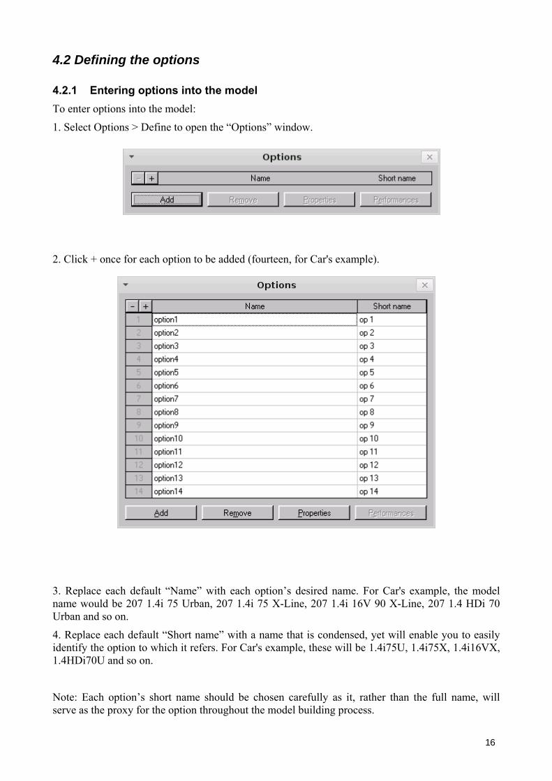
1. Select Options > Define to open the “Options” window.
2. Click + once for each option to be added (fourteen, for Car's example).
3. Replace each default “Name” with each option’s desired name. For Car's example, the model name would be 207 1.4i 75 Urban, 207 1.4i 75 X-Line, 207 1.4i 16V 90 X-Line, 207 1.4 HDi 70 Urban and so on.
4. Replace each default “Short name” with a name that is condensed, yet will enable you to easily identify the option to which it refers. For Car's example, these will be 1.4i75U, 1.4i75X, 1.4i16VX, 1.4HDi70U and so on.
Note: Each option’s short name should be chosen carefully as it, rather than the full name, will serve as the proxy for the option throughout the model building process.

17
4.3 Building the value tree and defining criteria
4.3.1 Types of nodes and bases for comparison Each node in a MACBETH tree can be either a criterion node or a non-criterion node, depending on whether or not it will be used to evaluate the options’ attractiveness. A criterion node should be always associated with a “basis for comparison”, either a direct (see section 4.3.3) or an indirect one (see section 4.3.4).
Note: To structure a MACBETH tree before defining which of its nodes are criterion nodes, enter each node as a non-criterion node.
Note: You can restructure a MACBETH tree by clicking and dragging any node to its new desired position in the tree. You should remember, however, that a criterion node can never be the parent of other criterion nodes.
4.3.2 Entering non-criterion nodes To enter a non-criterion node into the model:
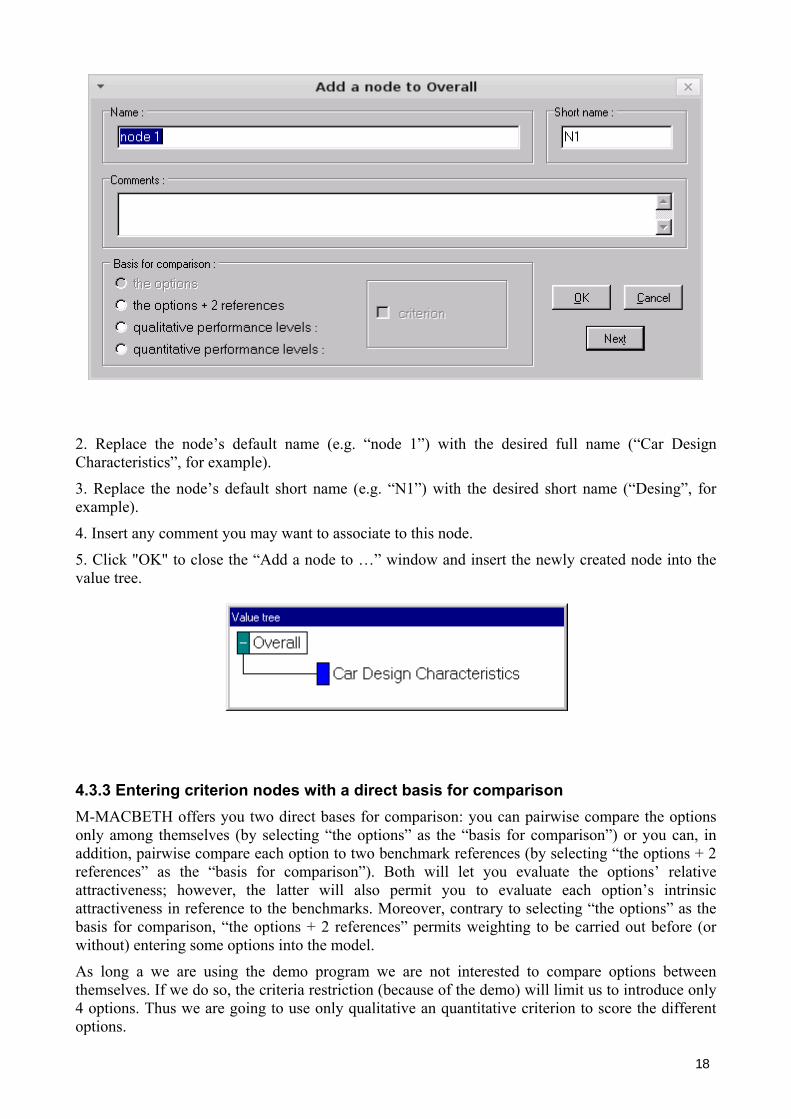
1. Right-click the parent node (“Overall”, for Car's example) and select “Add a node” from the pop-up menu to open the “Add a node to …” window.
18
2. Replace the node’s default name (e.g. “node 1”) with the desired full name (“Car Design Characteristics”, for example).
3. Replace the node’s default short name (e.g. “N1”) with the desired short name (“Desing”, for example).
4. Insert any comment you may want to associate to this node.
5. Click "OK" to close the “Add a node to …” window and insert the newly created node into the value tree.
4.3.3 Entering criterion nodes with a direct basis for comparison M-MACBETH offers you two direct bases for comparison: you can pairwise compare the options only among themselves (by selecting “the options” as the “basis for comparison”) or you can, in addition, pairwise compare each option to two benchmark references (by selecting “the options + 2 references” as the “basis for comparison”). Both will let you evaluate the options’ relative attractiveness; however, the latter will also permit you to evaluate each option’s intrinsic attractiveness in reference to the benchmarks. Moreover, contrary to selecting “the options” as the basis for comparison, “the options + 2 references” permits weighting to be carried out before (or without) entering some options into the model.
As long a we are using the demo program we are not interested to compare options between themselves. If we do so, the criteria restriction (because of the demo) will limit us to introduce only 4 options. Thus we are going to use only qualitative an quantitative criterion to score the different options.
19
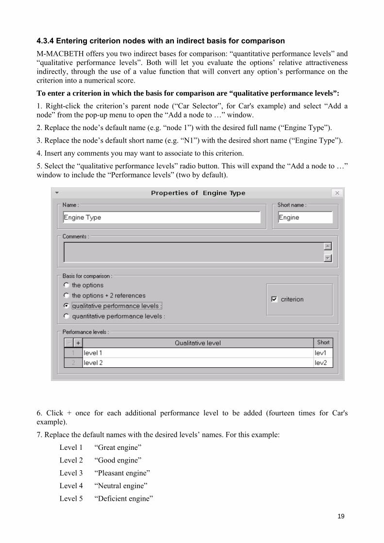
4.3.4 Entering criterion nodes with an indirect basis for comparison M-MACBETH offers you two indirect bases for comparison: “quantitative performance levels” and “qualitative performance levels”. Both will let you evaluate the options’ relative attractiveness indirectly, through the use of a value function that will convert any option’s performance on the criterion into a numerical score.
To enter a criterion in which the basis for comparison are “qualitative performance levels”: 1. Right-click the criterion’s parent node (“Car Selector”, for Car's example) and select “Add a node” from the pop-up menu to open the “Add a node to …” window.
2. Replace the node’s default name (e.g. “node 1”) with the desired full name (“Engine Type”).
3. Replace the node’s default short name (e.g. “N1”) with the desired short name (“Engine Type”).
4. Insert any comments you may want to associate to this criterion.
5. Select the “qualitative performance levels” radio button. This will expand the “Add a node to …” window to include the “Performance levels” (two by default).
6. Click + once for each additional performance level to be added (fourteen times for Car's example).
7. Replace the default names with the desired levels’ names. For this example:
Level 1 “Great engine”
Level 2 “Good engine”
Level 3 “Pleasant engine”
Level 4 “Neutral engine”
Level 5 “Deficient engine”
20
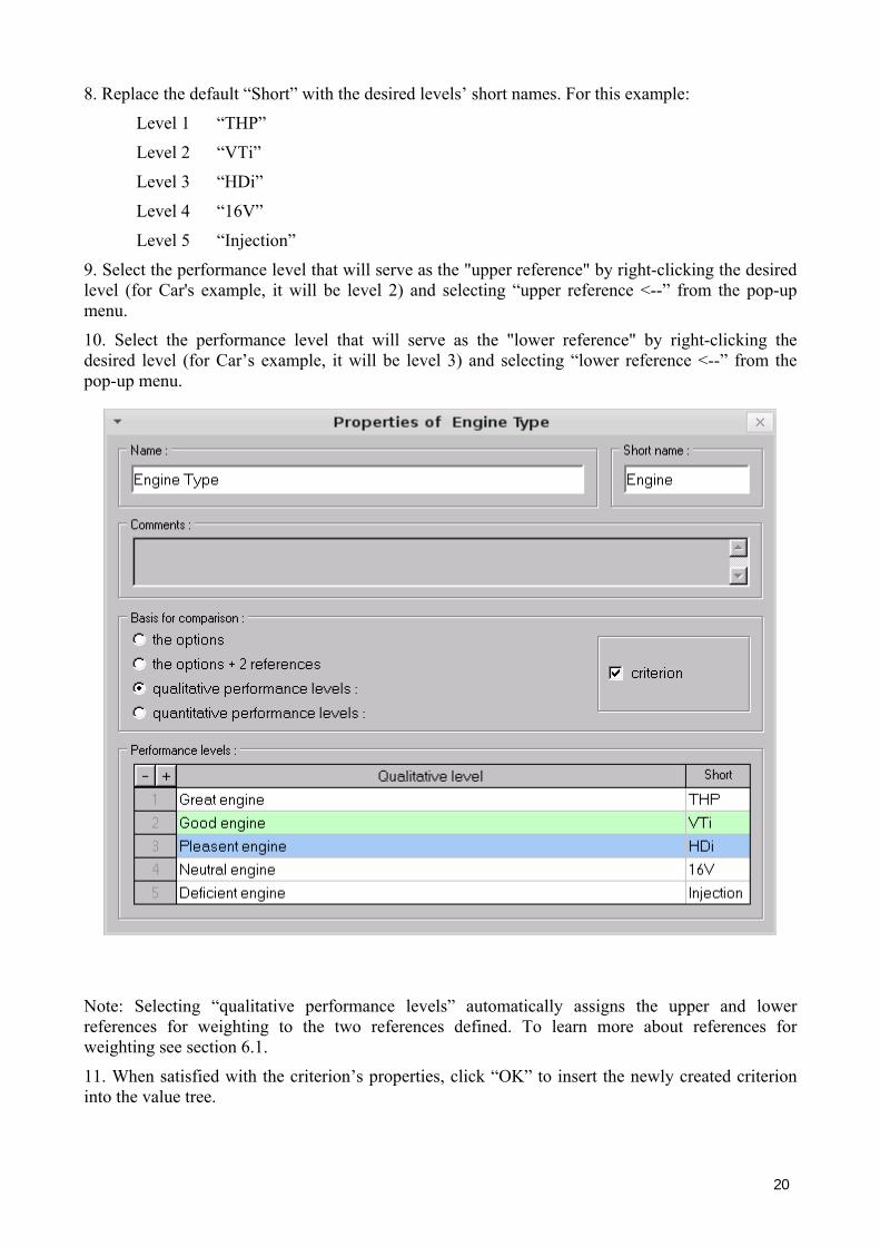
8. Replace the default “Short” with the desired levels’ short names. For this example:
Level 1 “THP”
Level 2 “VTi”
Level 3 “HDi”
Level 4 “16V”
Level 5 “Injection”
9. Select the performance level that will serve as the "upper reference" by right-clicking the desired level (for Car's example, it will be level 2) and selecting “upper reference <--” from the pop-up menu.
10. Select the performance level that will serve as the "lower reference" by right-clicking the desired level (for Car’s example, it will be level 3) and selecting “lower reference <--” from the pop-up menu.
Note: Selecting “qualitative performance levels” automatically assigns the upper and lower references for weighting to the two references defined. To learn more about references for weighting see section 6.1.
11. When satisfied with the criterion’s properties, click “OK” to insert the newly created criterion into the value tree.
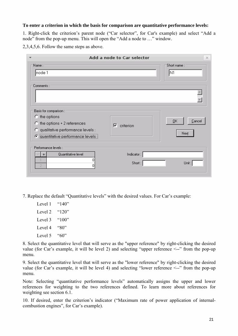
21
To enter a criterion in which the basis for comparison are quantitative performance levels: 1. Right-click the criterion’s parent node (“Car selector”, for Car's example) and select “Add a node” from the pop-up menu. This will open the “Add a node to …” window.
2,3,4,5,6. Follow the same steps as above.
7. Replace the default “Quantitative levels” with the desired values. For Car’s example:
Level 1 “140”
Level 2 “120”
Level 3 “100”
Level 4 “80”
Level 5 “60”
8. Select the quantitative level that will serve as the "upper reference" by right-clicking the desired value (for Car’s example, it will be level 2) and selecting “upper reference <--” from the pop-up menu.
9. Select the quantitative level that will serve as the "lower reference" by right-clicking the desired value (for Car’s example, it will be level 4) and selecting “lower reference <--” from the pop-up menu.
Note: Selecting “quantitative performance levels” automatically assigns the upper and lower references for weighting to the two references defined. To learn more about references for weighting see section 6.1.
10. If desired, enter the criterion’s indicator (“Maximum rate of power application of internal-combustion engines”, for Car’s example).

22
11. If desired, enter the default “Short” with an abbreviation of the criterion’s indicator (“Horsepower”, for Car’s example).
12. If desired, enter the criterion’s “Unit” (“CV”, for Car’s example).
13. When satisfied with the criterion’s properties, click "OK" to insert the newly created criterion into the model.
To complete Car's value tree, enter the following criterion nodes: “Accessory Pack”, another node with qualitative basis comparison, and “Fuel Consumption”, another node with quantitative basis for comparison.
23
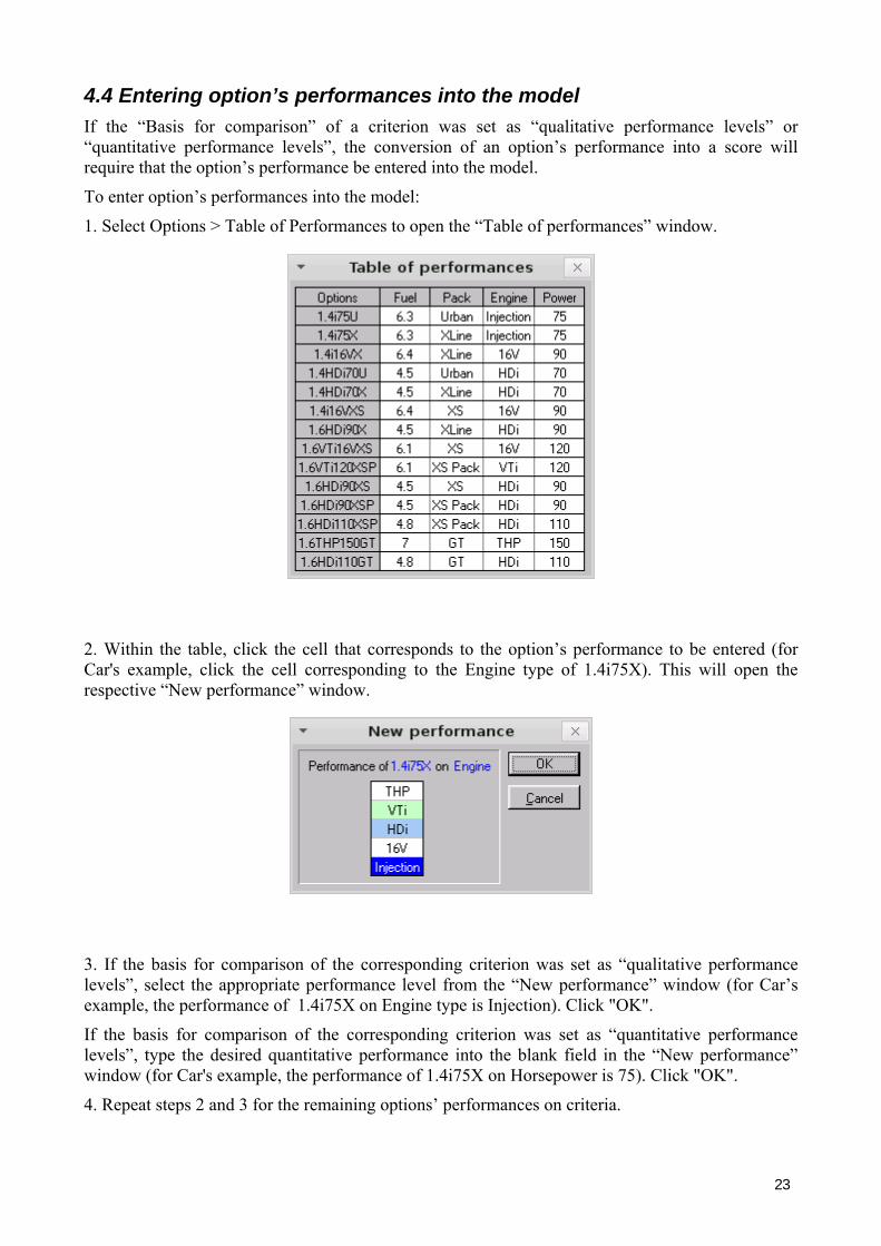
4.4 Entering option’s performances into the model If the “Basis for comparison” of a criterion was set as “qualitative performance levels” or “quantitative performance levels”, the conversion of an option’s performance into a score will require that the option’s performance be entered into the model.
To enter option’s performances into the model:
1. Select Options > Table of Performances to open the “Table of performances” window.
2. Within the table, click the cell that corresponds to the option’s performance to be entered (for Car's example, click the cell corresponding to the Engine type of 1.4i75X). This will open the respective “New performance” window.
3. If the basis for comparison of the corresponding criterion was set as “qualitative performance levels”, select the appropriate performance level from the “New performance” window (for Car’s example, the performance of 1.4i75X on Engine type is Injection). Click "OK".
If the basis for comparison of the corresponding criterion was set as “quantitative performance levels”, type the desired quantitative performance into the blank field in the “New performance” window (for Car's example, the performance of 1.4i75X on Horsepower is 75). Click "OK".
4. Repeat steps 2 and 3 for the remaining options’ performances on criteria.

24
Note: Any option’s performance on a criterion can be entered into the model at any time after the criterion has been defined.
Note: To highlight the profile of an option, click the respective cell on the first column of the “Table of performances”.

25
Chapter 5 - Scoring
5.1 Ranking within a criterion To rank within a criterion:
1. Within the value tree double-click the criterion for which you would like to rank either the options or the performance levels (depending on the criterion’s basis for comparison). This will open the matrix of MACBETH judgements for the selected criterion. For Car’s example, double-click “Fuel Consumption”.
2. Click and drag each of the options, or performance levels, to its desired position. For Car's example, arrange the options as follows: 4, 5, 6, 7, and 8.
3. To indicate that two options, or performance levels, are equally attractive with respect to the selected criterion, click one of the two cells that compare them (e.g. the cell that corresponds to the first option, or performance level, horizontally and the second one vertically) and select “no” from the MACBETH judgements bar.
4. Once you are satisfied with the ranking, click to open the pop-up menu and select “Validate ranking”. For Car's example, this will display the following window.

26
5.2 Qualitatively judging differences of attractiveness within a criterion To enter MACBETH judgements of difference of attractiveness within a criterion:
1. If the window with the matrix of judgements for the desired criterion is not already open, within the value tree double-click the criterion for which you would like to evaluate the difference of attractiveness between either options or performance levels (depending on the criterion’s basis for comparison). This will open the matrix of MACBETH judgements for the selected criterion.
2. Click the cell that corresponds to the comparison of the two desired options, or performance levels, ensuring that the more attractive option or performance level is highlighted in the selected cell’s row while the least attractive option or performance level is highlighted in the selected cell’s column.
3. Right-click the judgements bar, found on the right side of the window, to clear the cell for the judgement to be inserted.
4. Select the desired MACBETH judgement (or range of judgements) from the judgements bar
Note: Any of the seven semantic categories can be chosen as well as any sequence of judgements ranging from “very weak” to “extreme” (e.g. very weak to v. strong, weak to moderate, etc.). Since “no” represents equal attractiveness it cannot be combined with any of the other six categories of difference of attractiveness.
5. Repeat this process for each of the cells for which you would like to provide judgements.
Note: It is not necessary to provide a judgement for each cell in order to obtain scores.
Note: Keep in mind that, if the ranking has been validated: filling in the last column of the matrix is akin to comparing each of the options, or performance levels, to the least attractive one; filling in the first row is akin to comparing the most attractive option, or performance level, to each of the remanding options, or performance levels; filling in the diagonal above the main diagonal is akin to comparing each pair of options, or performance levels, that are consecutive in the ranking.
To alter a previously inserted MACBETH judgement:
1. Click the judgement that you would like to alter.
2. Right-click the judgements bar to clear the cell for the new judgement to be inserted.
3. Select the desired MACBETH judgement (or range of judgements) from the judgements bar.
5.3 Sorting out inconsistencies As each judgement is entered into a judgements matrix, M-MACBETH automatically verifies its compatibility with the judgements previously inserted into the matrix. If an incompatibility arises M-MACBETH will help you to sort it out. To sort out inconsistent judgements:

27
1. When an incompatible judgement is entered into a matrix of judgements, a confirmation window is displayed. For Car's example, within the matrix of judgements for “Engine Type”, enter the judgement “very strong” into the cell that compares VTi to HDi.
2. Click “Yes” to sort out the inconsistent judgements with the support of M-MACBETH. This will render the matrix inconsistent and open a window informing you of the number of ways that the software has found to obtain a consistent matrix with a minimal number of changes.
3. Click "OK" to analyse the M-MACBETH suggestions displayed in the inconsistent matrix.
4. Click the 4th button, from the tool bar at the bottom of the matrix window, to cycle through the suggestions displayed within the matrix’s window.
5. Click the 5th button accepts the current suggestion, indicated in the matrix by the filled in arrow(s) (and numbered at the bottom of the window). This will render the matrix consistent.
28
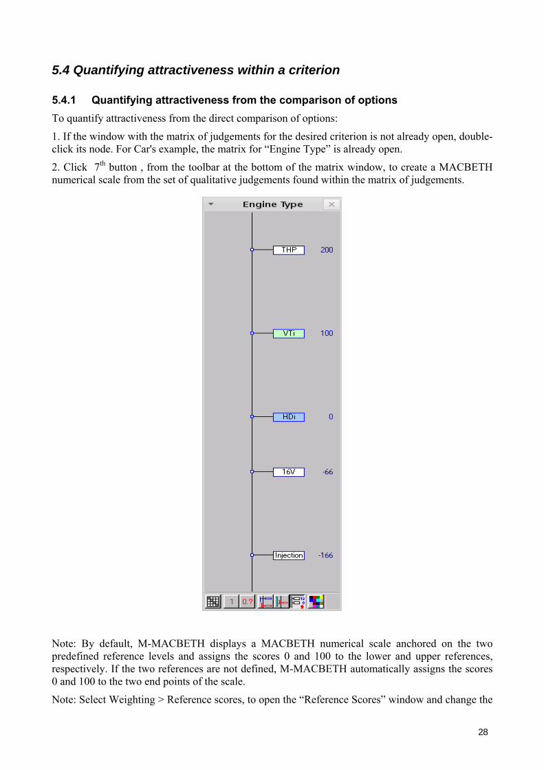
5.4 Quantifying attractiveness within a criterion
5.4.1 Quantifying attractiveness from the comparison of options To quantify attractiveness from the direct comparison of options:
1. If the window with the matrix of judgements for the desired criterion is not already open, double-click its node. For Car's example, the matrix for “Engine Type” is already open.
2. Click 7th button , from the toolbar at the bottom of the matrix window, to create a MACBETH numerical scale from the set of qualitative judgements found within the matrix of judgements.
Note: By default, M-MACBETH displays a MACBETH numerical scale anchored on the two predefined reference levels and assigns the scores 0 and 100 to the lower and upper references, respectively. If the two references are not defined, M-MACBETH automatically assigns the scores 0 and 100 to the two end points of the scale.
Note: Select Weighting > Reference scores, to open the “Reference Scores” window and change the
29
default reference scores for all criteria.
3. Click and drag any performance level whose score you want to adjust. This will open an interval within which the score of a performance level can be changed while keeping fixed the scores of the remaining performance levels and maintaining the compatibility with the matrix of judgements.
Note: To insert a precise numerical score, right-click the desired performance level and select “Modify score of …” from the pop-up menu.
Note: If the desired score is outside of the interval, consider revising some of the judgements found within the matrix of judgements.
4. To round the scores to integers, click “1” from the toolbar at the bottom of the scale window.
5. Repeat this process until you are satisfied with the differences within the scale.
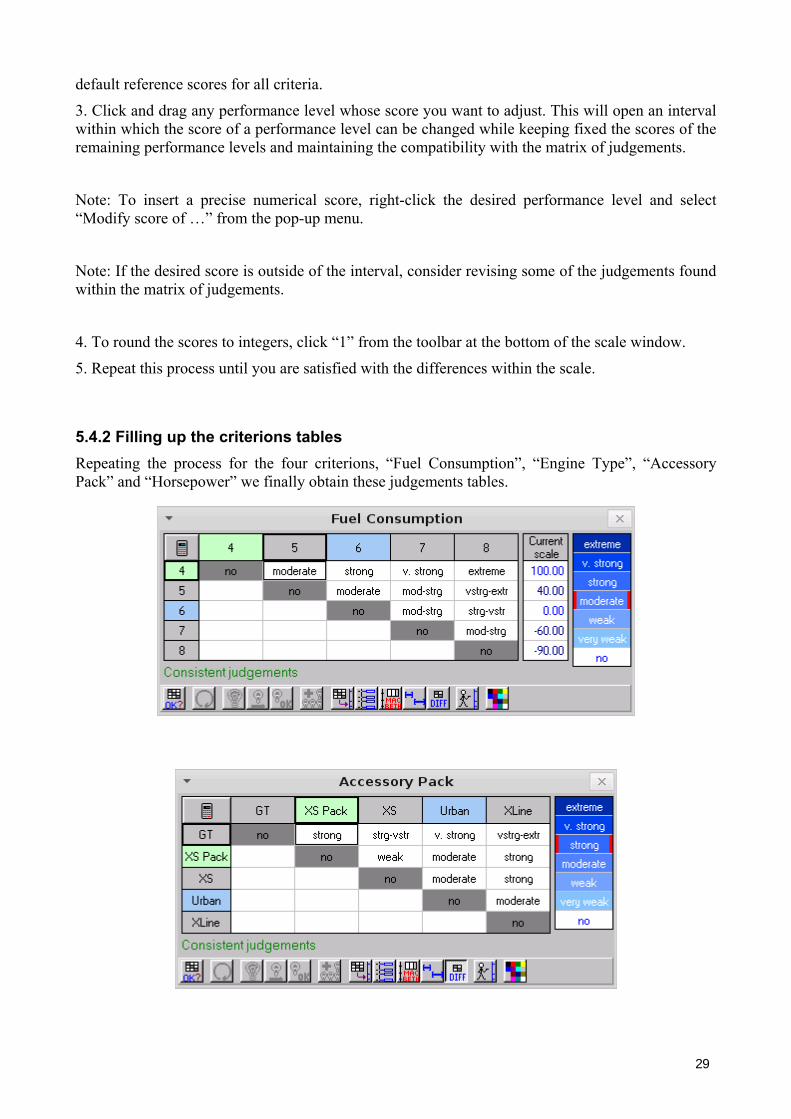
5.4.2 Filling up the criterions tables Repeating the process for the four criterions, “Fuel Consumption”, “Engine Type”, “Accessory Pack” and “Horsepower” we finally obtain these judgements tables.

30

31
Chapter 6 - Weighting
6.1 Weighting references To weight the model’s criteria, two weighting references (one “upper” and one “lower”) are required for each criterion.
To define an upper (or lower) weighting reference for a criterion (for Car’s example, the references were set when defining each of the three criteria – see section 4.3.3 and section 4.3.4):
1. Select Weighting > Weighting references… to open the “Weighting references” window.
Note: If a criterion’s "upper reference" has not been previously defined, none of the cells within its column is painted in light green; if a criterion’s "lower reference" has not been previously defined, none of the cells within its column is painted in blue.
2. Right-click the desired cell, in the criterion’s column, and select either “upper reference <-- …” (or “lower reference <-- …”) from the pop-up menu.
Note: In the left column (i.e. “Overall references”) of the “Weighting references” window: [ all lower ] represents an “overall reference” whose performances on all criteria are equal to their lower references; each criterion’s short name in brackets, [ short name ], represents an “overall reference” whose performance in the respective criterion is equal to its upper reference and whose performances in the remaining criteria are equal to their lower references ([ Fuel ], [ Engine ], [ Power ] and [ Pack ], for Car’s example).

32
Note: To highlight the profile of an overall reference, click its cell on the left column of the “Weighting references” window. To change the name of an overall reference, right-click its cell and select "Rename". Except for [ all lower ] this will automatically alter the “short name” of the respective criterion accordingly.
Note: Selecting “Weighting > Reference scores”, opens the “Reference scores” window, in which, besides the name of [ all lower ], one can also change the name of [ all upper ]; [ all upper ] represents an “overall reference” whose performances on all criteria are equal to their upper references.
6.2 Ranking the weights The ranking of criteria weights is determined by ranking the “overall references” in terms of their overall attractiveness.
To rank the weights (if upper and lower references have not yet been defined for all criteria, see section 6.1.
1. Select Weighting > Judgements to open the weighting matrix of judgements.
2. Click and drag each of the overall references to its desired position, until they are ranked in terms of decreasing (overall) attractiveness, from top to bottom. For Car’s example, arrange the overall references as follows: [ Fuel ], [ Engine ], [ Power ], [ Pack ] and [ all lower ].
Note: [ all lower ] must always be at the bottom of the ranking, as [ all lower ] is dominated by the remaining overall references, which are by definition more attractive than it in one criterion and equally attractive in all others.
3. To indicate that two overall references are equally attractive, click the cell that compare them (e.g. the cell that corresponds to the first overall reference horizontally and the second one vertically) and select “no” from the MACBETH judgements bar.

33
6.3 Qualitatively judging differences of overall attractiveness To enter qualitative judgements of difference of overall attractiveness between overall references:
1. If the weighting matrix of judgements is not already open, select Weighting > Judgements. For Car's example, the weighting matrix of judgements is already open.
2. Click the cell that corresponds to the comparison of the two desired overall references.
3. Right-click the judgements bar to clear the cell for the judgement to be inserted.
4. Select the desired MACBETH judgement (or range of judgements) from the judgements bar.
Note: Any of the seven semantic categories can be chosen as well as any sequence of judgements ranging from “very weak” to “extreme” (e.g. very weak to v. strong, weak to moderate, etc.). Since “no” represents equal attractiveness it cannot be combined with any of the other six categories of difference of attractiveness.
Note: Refer to section 4.3 to sort out any inconsistency that may occur.
5. Repeat this process for each of the cells for which you would like to provide judgements. For Car's example, introduce the weighting judgements as displayed in the following figure.
Note: It is not necessary to provide a judgement for each cell in order to quantify the weights.
6.4 Quantifying the weights To build a weights scale from the weighting matrix of judgements:
1. If the window with the weighting matrix of judgements is not already open, select
Weighting > Judgements. For Mary’s example, the matrix is already open.
2. Click the 7th button to create a MACBETH weighting scale.
3. Click and drag the top of the bar corresponding to the criterion whose weight you want to adjust.
This will open an interval within which the weight can be changed while maintaining the compatibility with the weighting matrix of judgements.

34
Note: To insert a precise numerical weight, right-click the respective bar and select “Modify weight of …” from the pop-up menu.
Note: If the desired weight is outside of the interval, consider revising some of the
judgements found within the weighting matrix of judgements.
4. To round the weights to integers, click “1” from the toolbar at the bottom of the weights window.

35
Chapter 7 - Analysing the Model’s Results
7.1 Overall scores Once the model has been built, you can see the model’s results in a concise results table.
Select Options > Table of scores to open the “Table of scores” window.
Note: [ all lower ] represents an overall reference whose performances on all criteria are equal to their lower references, while [ all upper ] represents an overall reference whose performances on all criteria are equal to their upper references. Both are benchmarks of intrinsic overall attractiveness.
Note: Select “Weighting > Reference scores” to change the name of [ all upper ] or [ all lower ].
Note: By default, the options are arranged in the order in which they appear within the “Options” window. Click “Overall” to rank the options in terms of decreasing overall attractiveness, from top to bottom.
7.2 Table of rankings The options’ overall scores can also be displayed separated by criterion through the “Table of rankings”.
Select Options > table of rankings to open the “Table of rankings” window.

36
7.3 Overall thermometer The options’ overall scores can also be displayed graphically through the “Overall thermometer”.
Select Options > Overall thermometer to open the “Overall thermometer” window.

37
7.4 Option’s profiles
In order to gain a more comprehensive understanding of the model’s results, M-MACBETH allows you to learn the extent to which an option’s scores contribute to its overall score.
To view an option’s profiles:
1. Select Options > Profiles and select the desired option from the pop-up menu (1.6THP150GT, for Car's example). This will open the “Option : profile” window.
Note: By default, the bars correspond to the option’s scores displayed in “Table of scores” window; since they do not take the criteria weights into consideration, they are not comparable. However, the bars provide you with a graphical view of the option’s scores relative to the benchmarks [ all lower ] and [ all upper ].
2. Check the box besides the weight symbol to display the bars that correspond to the weighted scores of the option.

38
Note: Each criterion bar in the weighted profile of the option corresponds to the product of the criterion weight and the option’s score on the criterion; the weighted profile therefore represents the individual contributions made by the option’s scores to the option’s overall score,
3. Check the first box to order the criteria bars according to their relevance to he option’s overall score (from greatest contribution to least).
7.5 Differences profiles
M-MACBETH allows you to explore the differences between the scores of any two options.
To view the differences profiles for any two options:
1. Select Options > Differences profiles to open the “Differences profiles” window.
Note: The information displayed compares the first of the two selected options to the second; therefore, positive differences (displayed by a green bar) point out the criteria for which the first of the two selected options outperformed the second option (Engine and Power, for Car's example). Likewise, any negative contribution (displayed by a red bar) indicates a criterion for which the second of the two selected options outperformed the first (Fuel, for Car’s example). Finally, a null difference means that the two options are indifferent in the criterion (Pack, for Car’s example).

39
Note: By default, the bars displayed within the “Differences profiles” window correspond to the differences of the options’ scores displayed in the “Table of scores” window; since they do not take the criteria weights into consideration, they are not comparable.
7.6 XY mapping
7.6.1 Comparing scores in two criteria or groups of criteria M-MACBETH allows you to display the model’s results in a two dimensional graph (“XY Map”), enabling you to compare the options’ scores in two criteria or groups of criteria. To compare the options’ scores in two criteria or groups of criteria:
1. Select Options > XY Map to open the “XY Map” window.
2. To select the two criteria or groups of criteria in which you want to compare the options’ scores, click at the right of each of the axes’ names and select each one of the desired nodes’ short names from the respective pop-up menu. For Car’s example, select “Fuel” and “Engine”.
3. Click to display the efficient frontier.
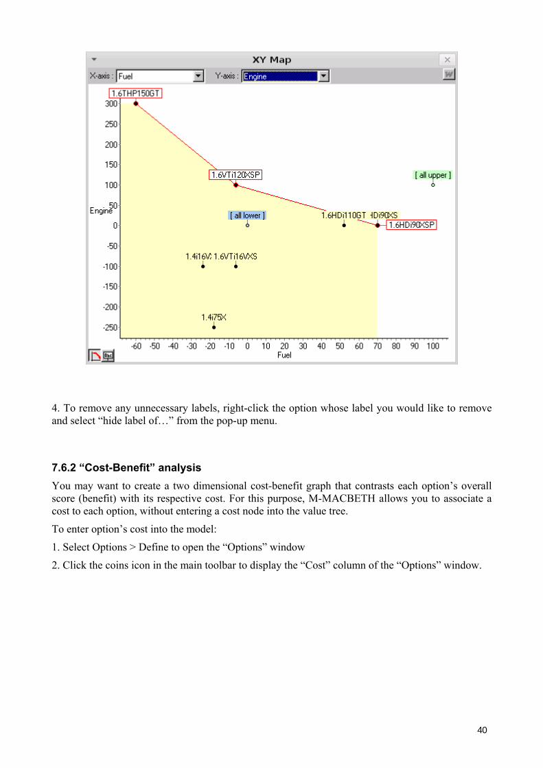
40
4. To remove any unnecessary labels, right-click the option whose label you would like to remove and select “hide label of…” from the pop-up menu.
7.6.2 “Cost-Benefit” analysis You may want to create a two dimensional cost-benefit graph that contrasts each option’s overall score (benefit) with its respective cost. For this purpose, M-MACBETH allows you to associate a cost to each option, without entering a cost node into the value tree.
To enter option’s cost into the model:
1. Select Options > Define to open the “Options” window
2. Click the coins icon in the main toolbar to display the “Cost” column of the “Options” window.

41
3. Double-click the cell of the “Cost” column that corresponds to the option’s cost to be entered (for Car’s example, click the cell corresponding to the cost of 1.4i75U). This will open the respective “Properties” window.
4. Within the “Properties” window, replace the default cost (0) by the desired one (for Car’s example, the cost of 1.4i75U is 12268€). Click “OK”.
5. Repeat steps 3 and 4 for the remaining options’ costs. For Car's example the options’ costs are indicated in Table 1.

42
To compare the options’ overall scores to their respective costs:
1. Select Options > XY Map to open the “XY Map” window.
2. Click at the right of each of the axes’ names and select “Cost” and “Car selector” from the respective pop-up menu.
Note: You may click the bottom right button to revert the order in which the costs are displayed.
3. To remove any unnecessary labels, right-click the option whose label you would like to remove and select “Hide label of …” from the pop-up menu.

43
Chapter 8 - Sensitivity and Robustness Analyses
8.1 Sensitivity Analyses
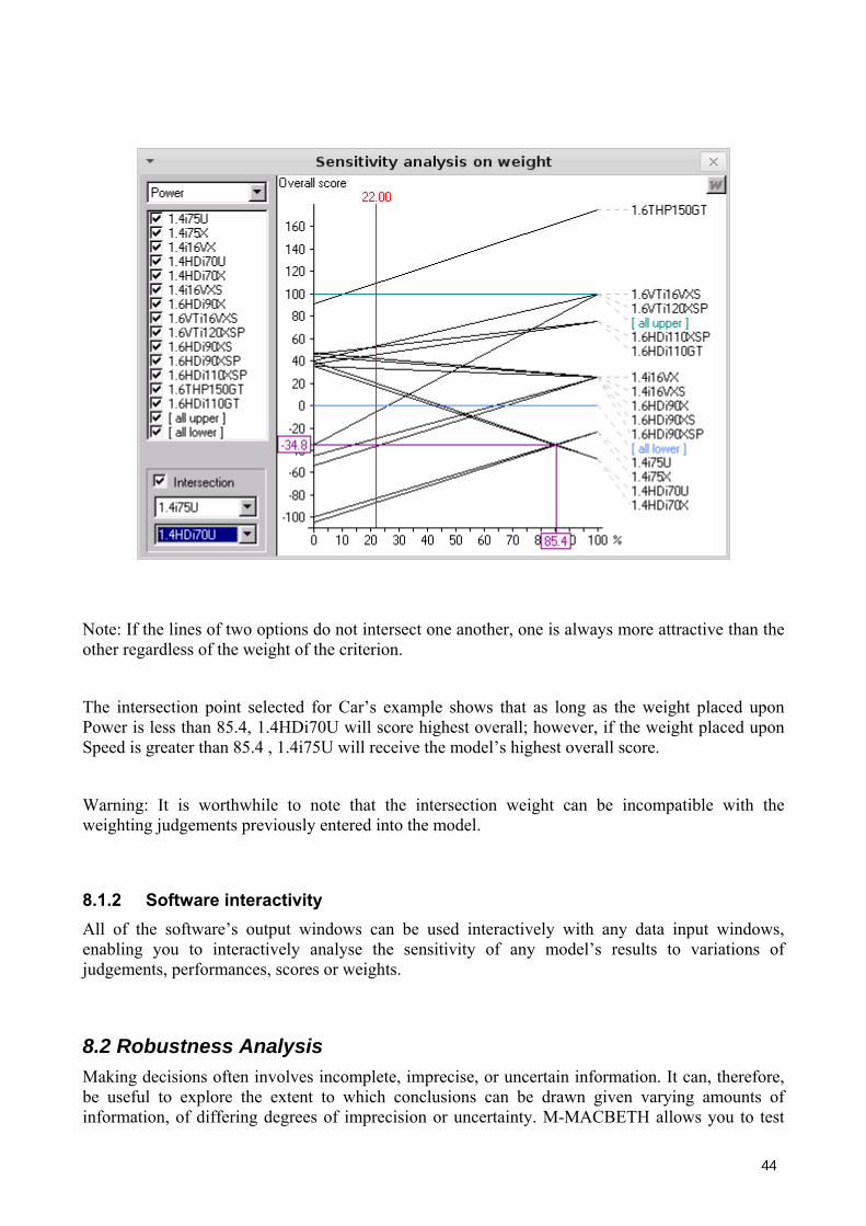
8.1.1 Sensitivity Analysis on a criterion weight Sensitivity analysis on a criterion weight allows you to visualise the extent of which the model’s recommendation would change as a result of changes made to the weight of the criterion.
To perform sensitivity analysis on weight:
1. Select Weighting > Sensitivity analysis on weight to open the “Sensitivity analysis on weight” window.
2. To select the criterion for which you would like to analyse the effects of a change in its weight on the options’ overall scores, click at the upper left corner of the window and select the criterion’s short name from the list (Power, for Car’s example).
Note: Each option’s line in the graph shows the variation of the option’s overall score when the criterion weight varies from 0 to 100%.
Note: The vertical red line on the following figure represents the current weight of the criterion (22.00 for Mary's example).
3. Remove from the graph any option’s line by unchecking its check box (for Mary’s example, remove [ all upper ] and [ all lower ]).
4. To find the weight associated with the intersection of any two of the options’ lines (i.e. the weight necessary to swap their rank in overall attractiveness), check the box intersection and select the two options to be compared from the pop-up menus that appear when clicking (1.4i75U and 1.4HDi70U, for Car's example).
44
Note: If the lines of two options do not intersect one another, one is always more attractive than the other regardless of the weight of the criterion.
The intersection point selected for Car’s example shows that as long as the weight placed upon Power is less than 85.4, 1.4HDi70U will score highest overall; however, if the weight placed upon Speed is greater than 85.4 , 1.4i75U will receive the model’s highest overall score.
Warning: It is worthwhile to note that the intersection weight can be incompatible with the weighting judgements previously entered into the model.
8.1.2 Software interactivity All of the software’s output windows can be used interactively with any data input windows, enabling you to interactively analyse the sensitivity of any model’s results to variations of judgements, performances, scores or weights.
8.2 Robustness Analysis Making decisions often involves incomplete, imprecise, or uncertain information. It can, therefore, be useful to explore the extent to which conclusions can be drawn given varying amounts of information, of differing degrees of imprecision or uncertainty. M-MACBETH allows you to test

45
this through its “robustness analysis” function. The following symbols will be used within the “Robustness analysis” window:
represents “dominance”: an option dominates another if it is at least as attractive as the other in all criteria and it is more attractive than the other in at least one criterion.
+ represents “additive dominance”: an option additively dominates another if it is always found to be more attractive than the other through the use of an additive model under a set of information constraints.
To explore the extent to which conclusions can be drawn given varying amounts of information:
1. Select Options > Robustness analysis to open the “Robustness analysis” window.
Note: M-MACBETH organises the information entered into the model into three types (“ordinal”, “MACBETH” and “cardinal”) and two sections (“Local information” and “Global information”). Ordinal information refers only to rank, thereby excluding any information pertaining to differences of attractiveness (strength of preference). MACBETH information includes the semantic judgements entered into the model; however, it does not distinguish between any of the possible numerical scales compatible with those judgements. Cardinal information denotes the specific scale validated by the decision maker. Local information is all information specific to a particular criterion, whereas global information pertains to the model’s weights.
Note: By default the robustness analysis process begins only with the consideration of local and global ordinal information.
2. Click the upper left corner to organise the options so that all the symbols are displayed in the upper part of the table.
3. To include local MACBETH information in the analysis, click the check box within the “Local information” section below “MACBETH” for each desired criterion. For Mary’s example, check each criterion’s “MACBETH” check box.

46
4. To add any of the remaining types of information, click the check box within the desired section, under the desired column. For Car’s example, include all local information as well as MACBETH global information.
For Car's example, the + in the following figure shows that without cardinal global information we can conclude that 1.6HDi90X additively dominates 1.4HDi70U.
For Car's example, the following figure shows that we cannot conclude that 1.6THP150GT is the best car without the cardinal global information.
To explore all the conclusions in the robustness tables check the cardinal box in global information

47
Chapter 9 – Analysis of countries using M-Macbeth
9.1 Data Set Characteristics
We have chosen a dataset about country information to make all the tests. The general information that it contains is: name, population, airport number, navigable river existence, climate, density, fertility, GDP and area.
We created our owd data bse with 80 countries (including Spain). Next picture shows a world map representing the selected countries:
(from http://www.world66.com/myworld66/visitedCountries )
Next table contains the information that we introduce in the M-MacBeth Software:
Country Population GDP Airports Area Afghanistan 29928987 800 47 Mig Albania 3563112 4900 11 Molt petit Algeria 32531853 7300 137 Molt gran Andorra 70549 26800 0 Molt petit Angola 11827315 2500 243 Gran Argentina 39537943 13600 1334 Molt gran Armenia 2982904 5100 16 Molt petit Australia 20090437 32000 448 Molt gran Austria 8184691 32900 55 Molt petit Azerbaijan 7911974 4600 50 Molt petit Bahrain 688345 20500 4 Molt petit Bangladesh 144319628 2100 16 Molt petit Belarus 10300483 7600 133 Petit Belgium 10364388 31800 43 Molt petit Benin 7649360 1200 5 Molt petit Bolivia 8857870 2700 1065 Gran Bosnia and Herzegovina 4430494 6800 27 Molt petit Botswana 1640115 10100 85 Mig Brazil 186112794 8500 4136 Molt gran Brunei 372361 23600 2 Molt petit Bulgaria 7450349 9000 213 Molt petit Burkina Faso 13491736 1200 33 Petit Burma 46996558 1800 78 Mig Cambodia 13636398 2100 20 Molt petit Cameroon 16988132 2000 47 Mig Canada 32805041 32800 1326 Molt gran

48
Cape Verde 418224 6200 7 Molt petit Central African Republic 4237703 1200 50 Mig Chad 9657069 1900 50 Gran Chile 15980912 11300 364 Mig China 1306313812 6200 472 Molt gran Colombia 42954279 7100 980 Gran Congo, Democratic Republic of the 60764490 800 230 Molt gran Congo, Republic of the 3602269 800 32 Petit Costa Rica 4016173 10000 149 Molt petit Cote d'Ivoire 17298040 1400 37 Petit Croatia 4495904 11600 68 Molt petit Cuba 11346670 3300 170 Molt petit Cyprus 780133 21600 17 Molt petit Czech Republic 10241138 18100 120 Molt petit Denmark 5432335 33500 97 Molt petit Dominican Republic 9049595 6500 31 Molt petit Ecuador 13363593 3900 205 Petit Egypt 77505756 4400 87 Molt petit El Salvador 6704932 5100 73 Molt petit Equatorial Guinea 529034 50200 4 Molt petit Eritrea 4669638 1000 17 Molt petit Estonia 1332893 16400 29 Molt petit Ethiopia 73053286 800 83 Gran Finland 5223442 30300 148 Petit France 60656178 29900 478 Mig Gabon 1394307 5800 56 Petit Gambia, The 1595086 1900 1 Molt petit Georgia 4677401 3400 30 Molt petit Germany 82431390 29700 550 Petit Ghana 21946247 2500 12 Petit Greece 10668354 22800 80 Molt petit Greenland 56375 20000 14 Molt gran Guatemala 12013907 4300 452 Molt petit Guinea 9452670 2200 16 Petit Guyana 765283 3900 49 Petit Haiti 8121622 1600 13 Molt petit Honduras 7167902 2900 115 Molt petit Hungary 10006835 15900 44 Molt petit Iceland 296737 34600 98 Molt petit India 1080264388 3400 333 Molt gran Indonesia 241973879 3700 667 Gran Iran 68017860 8100 305 Gran Iraq 26074906 3400 111 Mig Ireland 4015676 34100 36 Molt petit Israel 6276883 22200 51 Molt petit Italy 58103033 28300 134 Petit Jamaica 2735520 4300 35 Molt petit Japan 127417244 30400 174 Petit Jordan 5759732 4800 17 Molt petit Kazakhstan 15185844 8700 314 Molt gran Kenya 33829590 1200 221 Mig Korea, North 22912177 1800 78 Molt petit Korea, South 48640671 20300 179 Molt petit Spain 40341462 25100 156 Mig

49
Due to MACBETH limitations to import data from outside files (for instance, Excel files or text files), we have to introduce every alternatives by hand.
Also, due to the deficiencies of the demo version, we could work only with 4 criteria (we chose them to consider the most suitable to the decision making): GDP (Gross Domestic Product), Area, Population and Airport Number.
To doing these tests, we suppose the need of taking a decision as regards a selection of the best country to set a company up:
9.2 Data Introduction
CRITERIA: There are four criteria:
GDP (Gross Domestic Product: euros): criterion node with five quantitative performance levels:
We defined the top level as the number 1 (20.000) and as the lower level, the number 4 (2.000), it means that the top level is consider like the value 100 and the inferior level like 0. Supposing higher or lower values to these limits, the marks will be higher to 100 or negatives.

50
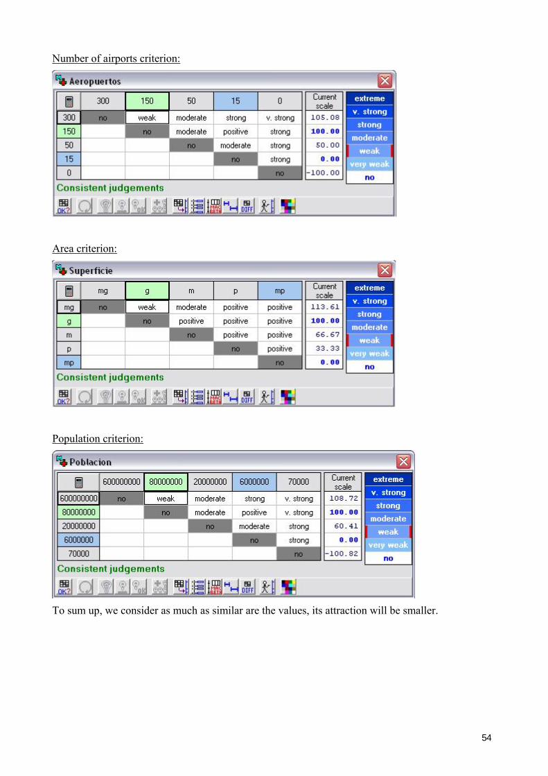
Airports Number (units): criterion node with five qualitative performance levels:
We have defined as the top level, the number 2 (150) and as the inferior level, the number 4 (15).
Area (discrete units): criterion node with five quantitative performance levels:
We have defined as the highest level, the number 2 (“gran”) and as the lowest level, the number 5 (“molt petit”).

51
Population (number of inhabitants) : criterion node with five quantitative performance levels:
We have defined as the top level, the number 2 (80.000.000) and as the inferior level, the number 4 (6.000.000).
WEIGHTS OF CRITERIA: In our opinion, we consider GDP (Gross Domestic Product) and Population as the most important criteria and we assigned them a weight of 45% and 35%, respectively. Airport Number with a 15% and Area with a 5% are the less important ones.
52
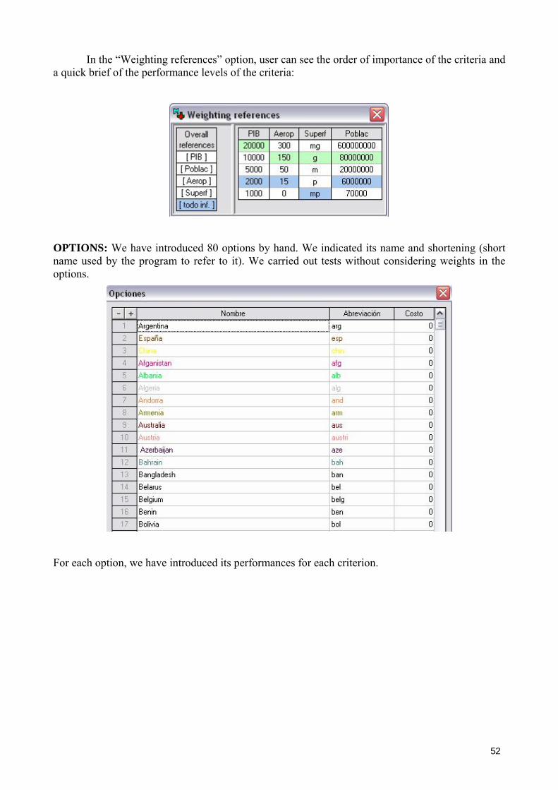
In the “Weighting references” option, user can see the order of importance of the criteria and a quick brief of the performance levels of the criteria:
OPTIONS: We have introduced 80 options by hand. We indicated its name and shortening (short name used by the program to refer to it). We carried out tests without considering weights in the options.
For each option, we have introduced its performances for each criterion.

53
In this image, we can see the list of countries (our options) on the left and the short name of the criteria on which we work at the top.
JUDGEMENTS: We have introduced all the judgements for each criterion depending on the attractive categories (very weak, weak, moderate, strong, very strong, extreme). So, we have the following judgements:
GDP criterion:
If we compare the first category (20.000) with the rest of categories, its preference is:
Moderate against 10.000
Strong against 5.000
Very Strong against 2.000
Extreme against 1.000
In other words, we prefer the extreme manner the category “20.000” against category “1.000”, the very strong manner against the category “2.000”, the strong manner against the category “5.000” and the moderate manner against “10.000”.
54
Number of airports criterion:
Area criterion:
Population criterion:
To sum up, we consider as much as similar are the values, its attraction will be smaller.

55
9.3 Results
9.3.1 Overall Scores If the user chooses this option, a global table will be shown with all the results of the attraction calculations of each option as regards the rest of criteria. The final mark is also in the second column (in yellow colour).
In the next image, the results of the best ten countries are shown. The eighth row is the superior level (predefined by the user: [todo sup.]). Therefore, there are seven countries which exceed this level: Canada, Germany, Japan, France, Australia, Italy and Brazil (They will be the most suitable to set a company up).
In conclusion, the best country will be Canada.
The classification of all the options is: Options Overall DGP Airports Area Population
can 127.31 142.66 139.83 113.61 104.16 ger 113.26 132.33 113.55 33.33 100.04 jap 112.67 134.66 100.81 33.33 100.80 fra 110.38 133.00 111.11 66.67 87.24 aus 106.36 140.00 110.09 113.61 60.47 ita 102.86 127.66 92.00 33.33 85.55 bra 102.05 56.67 234.99 113.61 101.78 [ todo sup. ] 100.00 100.00 100.00 100.00 100.00 esp 96.85 117.00 100.20 66.67 73.83 kors 88.36 101.00 100.98 0.00 79.31 arg 87.75 78.67 140.10 113.61 73.30 chin 83.11 41.33 110.91 113.61 120.56 iran 77.32 54.00 105.25 100.00 92.09 austri 75.52 143.00 52.50 0.00 9.43 belg 75.29 139.33 40.00 0.00 18.83 den 72.90 145.00 73.50 0.00 -9.65 fin 72.34 134.33 99.00 33.33 -13.20 col 71.96 47.33 128.11 100.00 75.56 ind 69.48 15.55 106.20 113.61 116.77 indo 67.08 18.89 117.51 100.00 102.72 chi 66.45 71.00 107.25 66.67 43.07

56
gree 66.00 109.33 65.00 0.00 20.14 alg 65.64 48.67 93.50 113.61 68.68 kaz 61.49 58.00 105.55 113.61 39.64 cze 61.31 93.67 85.00 0.00 18.30 ire 58.84 147.00 30.00 0.00 -33.74 egy 56.70 26.66 68.50 0.00 98.35 isr 56.29 107.33 50.50 0.00 1.19 hun 51.12 86.33 41.43 0.00 17.29 iraq 44.95 15.55 80.50 66.67 64.42 bel 44.69 50.67 91.50 33.33 18.56 bul 44.51 60.00 102.13 0.00 6.26 ice 44.06 148.66 74.00 0.00 -96.97 ecu 37.57 21.11 101.86 33.33 31.77 gua 37.22 25.55 110.91 0.00 25.95 burm 36.31 -8.89 64.00 66.67 78.22 ban 36.09 1.11 1.43 0.00 101.08 cost 33.12 66.67 99.50 0.00 -33.73 bol 32.46 7.78 130.99 100.00 12.33 croa 32.30 72.00 59.00 0.00 -25.57 ang 31.77 5.56 103.15 100.00 25.14 Cub 29.68 14.44 100.68 0.00 23.07 DRC 27.65 -53.33 102.71 113.61 87.31 dom 27.53 43.33 22.86 0.00 13.16 korn 27.42 -8.89 64.00 0.00 62.33 ken 27.03 -35.55 102.40 66.67 69.54 came 26.79 0.00 45.71 66.67 47.41 els 25.59 34.00 61.50 0.00 3.04 eth 24.37 -53.33 66.50 100.00 95.42 aze 23.39 28.89 50.00 0.00 8.25 gha 22.76 5.56 -20.00 33.33 61.69 hon 18.64 10.00 82.50 0.00 5.04 bot 17.67 67.00 67.50 66.67 -74.13 cyp 16.77 105.33 2.86 0.00 -88.75 stonia 14.83 88.00 20.00 0.00 -79.35 cha 14.36 -4.44 50.00 66.67 15.78 green 14.31 100.00 -6.67 113.61 -101.05 bos 13.63 45.33 17.14 0.00 -26.68 cam 13.10 1.11 7.14 0.00 32.95 jor 13.00 31.11 2.86 0.00 -4.08 Cote 11.44 -26.66 31.43 33.33 48.75 afg 9.63 -53.33 45.71 66.67 66.96 gui 8.10 2.22 1.43 33.33 14.90 and 4.92 122.66 -100.00 0.00 -100.81 bru 3.91 112.00 -86.67 0.00 -95.68 bah 3.14 101.67 -73.33 0.00 -90.31 geo 2.34 15.55 21.43 0.00 -22.49 bur 0.84 -35.55 25.71 33.33 32.33 [ todo inf. ] 0.00 0.00 0.00 0.00 0.00 gab -0.39 38.66 53.00 33.33 -78.30 arm -2.44 34.00 1.43 0.00 -51.30 jam -3.64 25.55 28.57 0.00 -55.50 alb -4.00 32.22 -26.67 0.00 -41.43 hai -6.80 -17.78 -13.33 0.00 9.15 guy -12.70 21.11 48.57 33.33 -89.00 car -15.65 -35.55 50.00 66.67 -29.96 cab -22.62 41.33 -53.33 0.00 -94.90 ben -23.51 -35.55 -66.67 0.00 7.12 eri -27.49 -44.44 2.86 0.00 -22.62 EcuGui -27.96 34.66 -73.33 0.00 -93.02 RC -34.62 -53.33 24.29 0.00 -40.77 gam -42.21 -4.44 -93.33 0.00 -74.89

57
9.3.2 Overall Thermometer In this image, an order country list is shown to the user in accordance with its marks (it maintains a proportional gap between every countries).

58
9.3.3 Option’s Profiles
MACBETH can show a chart for each alternative which summarizes its values for each criterion.
In this concrete case, Andorra has a GDP level higher than maximum (green slash), an area equals to the lower level (molt petit) and negatives values in airport number and population (red slashes).
The best profiles (those who are over the upper limit) are:
1st : Canada
2nd : Germany

59
3rd : Japan
4th: France
5th : Australia
6th : Italy

60
7th : Brazil
The worst profiles (those who are under the lower limit) are in inverse order:
1st : Gabon
2nd : Armenia
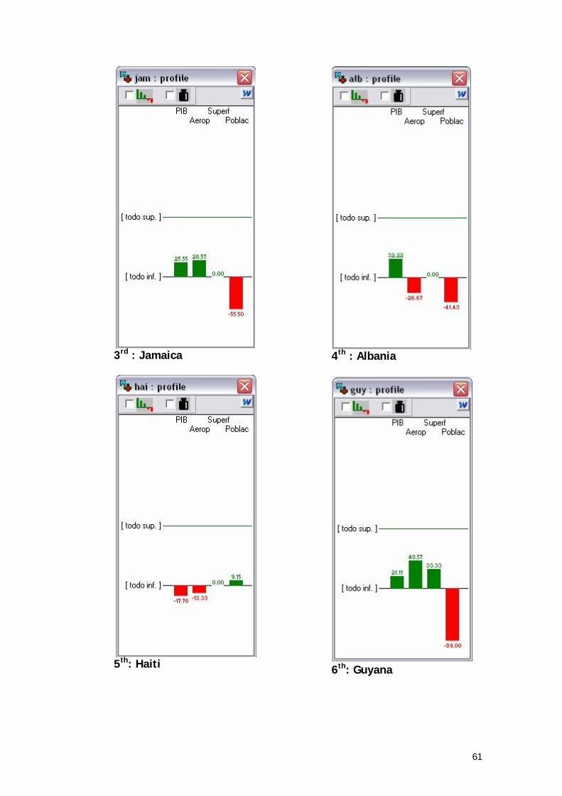
61
3rd : Jamaica
5th: Haiti
4th : Albania
6th: Guyana

62
7th: Central African Republic
9th : Benin
8th : Cape Verde
10th : Eritrea

63
11th : Equatorial Guinea
12th : Republic of the Congo
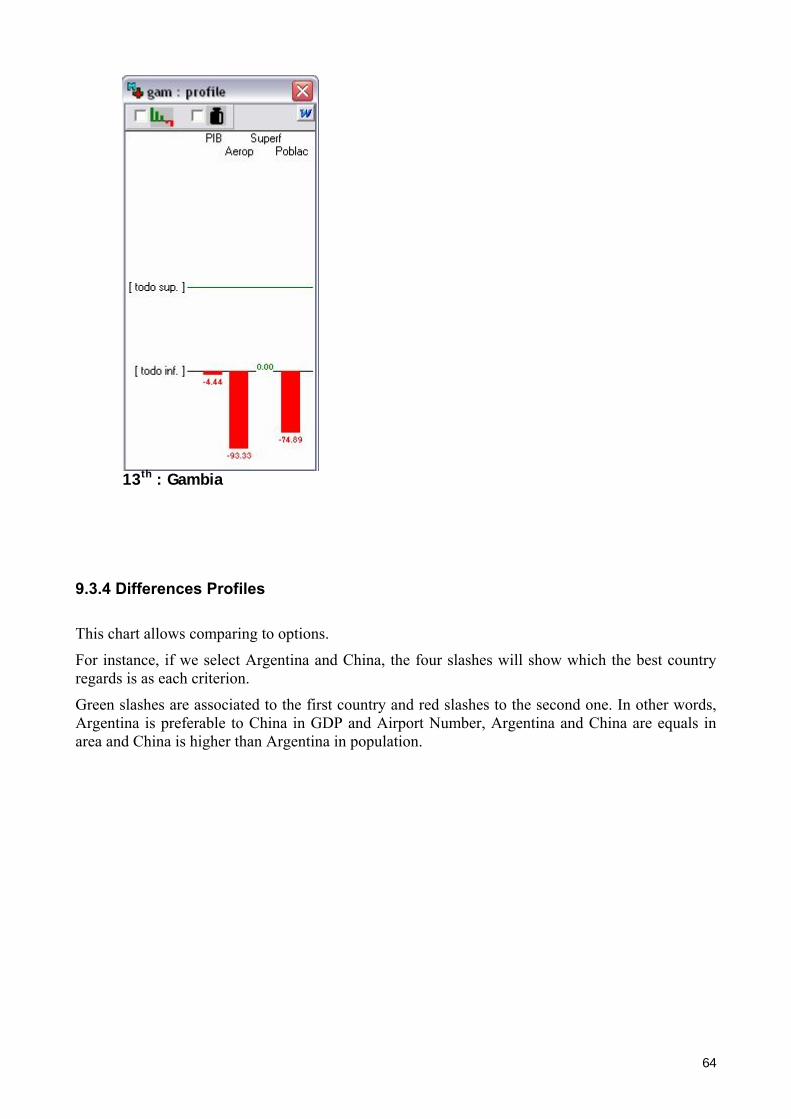
64
13th : Gambia
9.3.4 Differences Profiles This chart allows comparing to options.
For instance, if we select Argentina and China, the four slashes will show which the best country regards is as each criterion.
Green slashes are associated to the first country and red slashes to the second one. In other words, Argentina is preferable to China in GDP and Airport Number, Argentina and China are equals in area and China is higher than Argentina in population.

65
Argentina Profile
China Profile
Differences Profile (Argentina vs. China)

66
If we analyse the best country (Canada) against the worst one (Gambia), the results will be clear:
Moreover, we compare Canada against Brazil (the first country over the upper limit):

67
Finally, we compare Gambia against the country which is immediately under the lower limit, Gabon:

68
9.3.5 XY Mapping
Users can see the distribution of the countries regards as two criteria.
In this image, the X criterion is GDP and the Y criterion is the Area. It’s curious that we can affirm that it doesn’t exist any relationship between these two criteria. The countries are scattered around the chart without any reason.
In the next image, the X criterion is Airports and the Y criterion is Population. In this case the relation between airports and population is proportional. It’s logical that countries with more population, also they have a number of airports higher.

69

70
9.3.6 Robustness Analysis
This table is used to analyse which conclusions can be extracted depending on different levels of local and global information:
The following symbols are used within this window:
represents “dominance”: an option dominates another if it is at least as attractive as the other
in all criteria and it is more attractive than the other in at least one criterion.
represents “additive dominance”: an option additively dominates another if it is always
found to be more attractive than the other through the use of an additive model under a set
of information constraints.
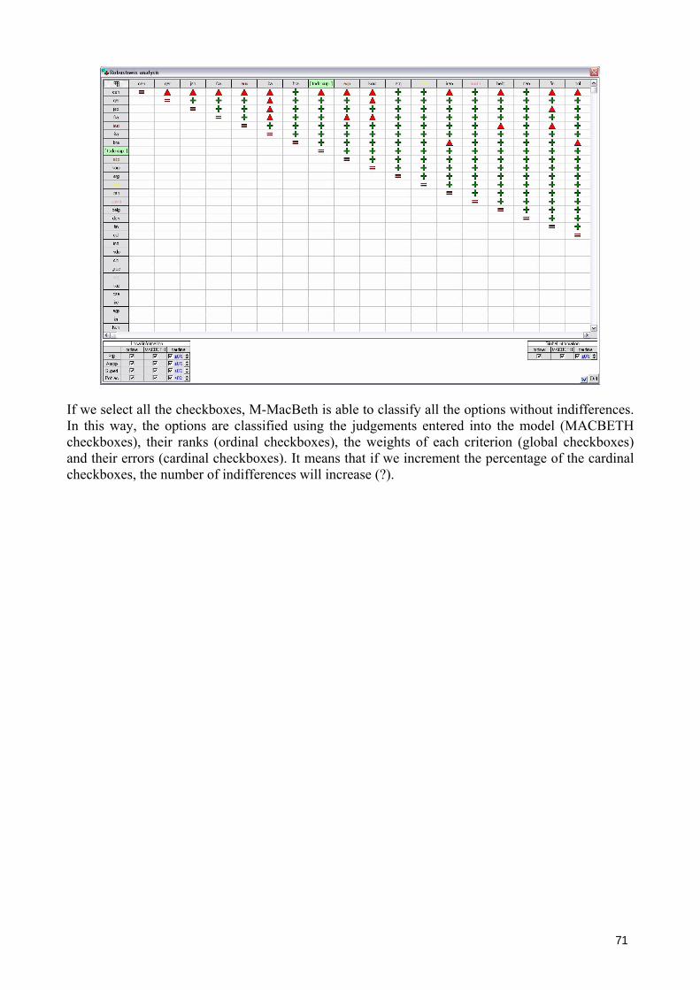
71
If we select all the checkboxes, M-MacBeth is able to classify all the options without indifferences. In this way, the options are classified using the judgements entered into the model (MACBETH checkboxes), their ranks (ordinal checkboxes), the weights of each criterion (global checkboxes) and their errors (cardinal checkboxes). It means that if we increment the percentage of the cardinal checkboxes, the number of indifferences will increase (?).
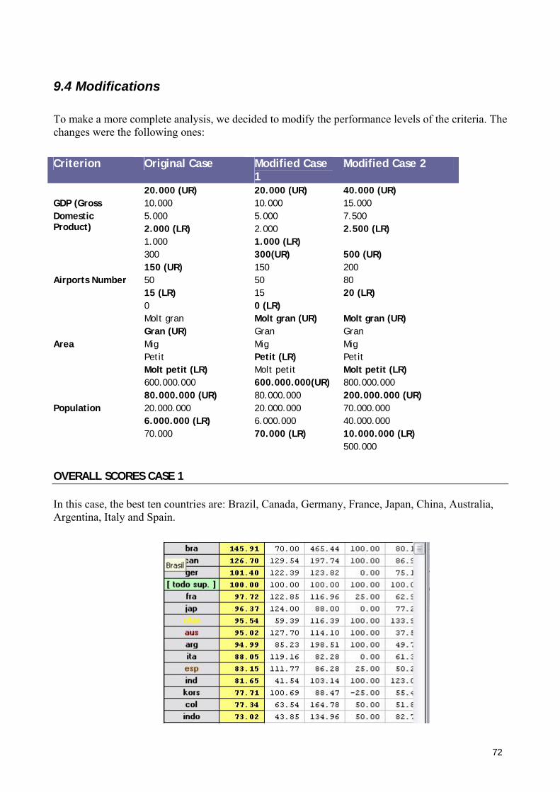
72
9.4 Modifications
To make a more complete analysis, we decided to modify the performance levels of the criteria. The changes were the following ones:
Criterion Original Case Modified Case
1 Modified Case 2
GDP (Gross Domestic Product)
20.000 (UR) 10.000 5.000 2.000 (LR) 1.000
20.000 (UR) 10.000 5.000 2.000 1.000 (LR)
40.000 (UR) 15.000 7.500 2.500 (LR)
Airports Number
300 150 (UR) 50 15 (LR) 0
300(UR) 150 50 15 0 (LR)
500 (UR) 200 80 20 (LR)
Area
Molt gran Gran (UR) Mig Petit Molt petit (LR)
Molt gran (UR) Gran Mig Petit (LR) Molt petit
Molt gran (UR) Gran Mig Petit Molt petit (LR)
Population
600.000.000 80.000.000 (UR) 20.000.000 6.000.000 (LR) 70.000
600.000.000(UR) 80.000.000 20.000.000 6.000.000 70.000 (LR)
800.000.000 200.000.000 (UR) 70.000.000 40.000.000 10.000.000 (LR) 500.000
OVERALL SCORES CASE 1
In this case, the best ten countries are: Brazil, Canada, Germany, France, Japan, China, Australia, Argentina, Italy and Spain.

73
In conclusion, the best country will be Brazil.
The modified classification of all the options is:
Options Overall DGP Airports Area Population bra 145.91 70.00 465.44 100.00 80.10 can 126.70 129.54 197.74 100.00 86.92 ger 101.40 122.39 123.82 0.00 75.12 [ todo sup. ] 100.00 100.00 100.00 100.00 100.00 fra 97.72 122.85 116.96 25.00 62.91 jap 96.37 124.00 88.00 0.00 77.28 chin 95.54 59.39 116.39 100.00 133.96 aus 95.02 127.70 114.10 100.00 37.56 arg 94.99 85.23 198.51 100.00 49.71 ita 88.05 119.16 82.28 0.00 61.31 esp 83.15 111.77 86.28 25.00 50.21 ind 81.65 41.54 103.14 100.00 123.09 kors 77.71 100.69 88.47 -25.00 55.40 col 77.34 63.54 164.78 50.00 51.85 indo 73.02 43.85 134.96 50.00 82.79 iran 72.86 68.15 100.48 50.00 67.51 austri 70.79 129.77 65.36 -25.00 5.85 belg 70.55 127.23 60.00 -25.00 11.69 den 68.86 131.16 74.36 -25.00 -7.18 fin 67.91 123.77 85.28 0.00 -9.82 chi 64.87 79.92 106.10 25.00 26.73 alg 63.44 64.46 82.93 100.00 45.33 gree 63.39 106.46 70.72 -25.00 12.50 kaz 63.03 70.92 101.33 100.00 24.60 ire 60.39 132.54 55.72 -25.00 -25.10 cze 59.68 95.61 79.28 -25.00 11.36 isr 57.88 105.08 64.50 -25.00 0.74 egy 57.41 49.23 72.22 -25.00 73.44 hun 53.84 90.54 60.62 -25.00 10.73 bol 52.34 36.16 172.88 50.00 7.66 ice 49.25 133.70 74.57 -25.00 -72.13 bul 49.04 72.31 91.71 -25.00 3.88 bel 48.09 65.85 82.07 0.00 11.52 iraq 47.08 41.54 77.36 25.00 41.30 GUA 46.66 48.46 116.39 -25.00 16.11 ban 45.76 31.54 43.47 -25.00 78.09 ecu 43.11 45.39 90.95 0.00 19.72 burm 42.38 24.62 70.29 25.00 54.37 croa 41.20 80.61 68.15 -25.00 -19.02 cost 40.72 76.92 85.50 -25.00 -25.09 ang 40.09 34.62 94.57 50.00 15.61 DRC 39.18 -6.15 93.33 100.00 62.98 dom 38.19 60.77 52.66 -25.00 8.17 cub 37.45 40.77 87.62 -25.00 14.32 els 36.25 54.31 69.22 -25.00 1.89 came 35.76 30.77 62.45 25.00 29.43

74
ken 35.43 6.15 92.47 25.00 46.14 eth 35.19 -6.15 71.36 50.00 70.66 korn 35.06 24.62 70.29 -25.00 39.32 aze 34.81 50.77 64.29 -25.00 5.12 gha 34.14 34.62 34.29 0.00 38.72 green 33.15 100.00 40.00 100.00 -75.17 cyp 32.22 103.69 44.08 -25.00 -66.02 bot 31.24 77.15 71.79 25.00 -55.14 hon 30.79 37.69 78.21 -25.00 3.13 stonia 30.38 91.69 51.43 -25.00 -59.03 bos 29.41 62.16 50.21 -25.00 -19.85 jor 29.25 52.31 44.08 -25.00 -3.04 cha 28.42 27.69 64.29 25.00 9.80 cam 27.75 31.54 45.92 -25.00 20.45 and 26.81 115.69 0.00 -25.00 -74.99 bru 25.74 108.31 5.71 -25.00 -71.18 Cote 25.36 12.31 56.33 0.00 30.26 gui 25.32 32.31 43.47 0.00 9.25 bah 24.83 101.15 11.43 -25.00 -67.18 afg 23.71 -6.15 62.45 25.00 43.71 geo 21.46 41.54 52.04 -25.00 -16.73 gab 19.06 57.54 65.58 0.00 -58.25 bur 18.89 6.15 53.88 0.00 20.07 arm 18.80 54.31 43.47 -25.00 -38.16 alb 18.43 53.08 31.43 -25.00 -30.82 jam 17.27 48.46 55.11 -25.00 -41.29 hai 15.56 18.46 37.15 -25.00 5.68 guy 10.70 45.39 63.68 0.00 -66.21 car 8.46 6.15 64.29 25.00 -22.29 cab 6.48 59.39 20.00 -25.00 -70.60 ben 5.50 6.15 14.29 -25.00 4.42 EcuGui 3.31 54.77 11.43 -25.00 -69.19 eri 1.30 0.00 44.08 -25.00 -16.83 [ todo inf. ] 0.00 0.00 0.00 0.00 0.00 RC -4.14 -6.15 53.27 -25.00 -30.33 gam -6.10 27.69 2.86 -25.00 -55.71

75
OVERALL THERMOMETER CASE 1 In the next image, the new classification is represented.
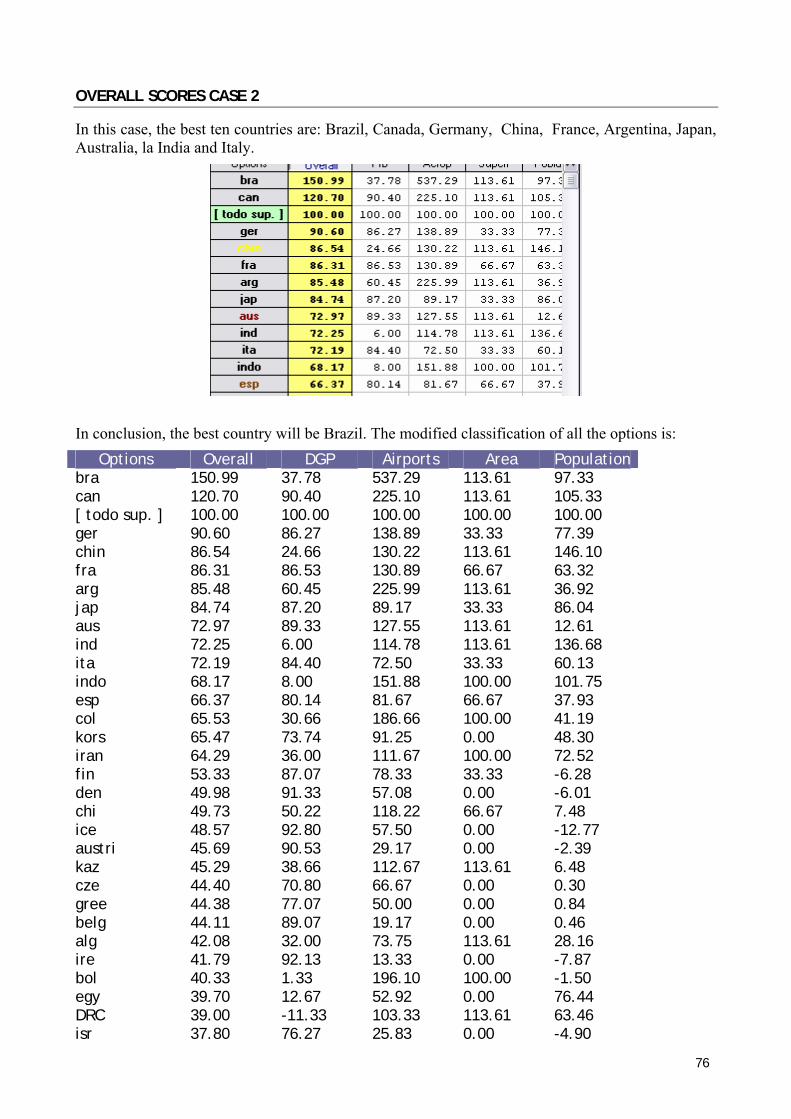
76
OVERALL SCORES CASE 2
In this case, the best ten countries are: Brazil, Canada, Germany, China, France, Argentina, Japan, Australia, la India and Italy.
In conclusion, the best country will be Brazil. The modified classification of all the options is: Options Overall DGP Airports Area Population
bra 150.99 37.78 537.29 113.61 97.33 can 120.70 90.40 225.10 113.61 105.33 [ todo sup. ] 100.00 100.00 100.00 100.00 100.00 ger 90.60 86.27 138.89 33.33 77.39 chin 86.54 24.66 130.22 113.61 146.10 fra 86.31 86.53 130.89 66.67 63.32 arg 85.48 60.45 225.99 113.61 36.92 jap 84.74 87.20 89.17 33.33 86.04 aus 72.97 89.33 127.55 113.61 12.61 ind 72.25 6.00 114.78 113.61 136.68 ita 72.19 84.40 72.50 33.33 60.13 indo 68.17 8.00 151.88 100.00 101.75 esp 66.37 80.14 81.67 66.67 37.93 col 65.53 30.66 186.66 100.00 41.19 kors 65.47 73.74 91.25 0.00 48.30 iran 64.29 36.00 111.67 100.00 72.52 fin 53.33 87.07 78.33 33.33 -6.28 den 49.98 91.33 57.08 0.00 -6.01 chi 49.73 50.22 118.22 66.67 7.48 ice 48.57 92.80 57.50 0.00 -12.77 austri 45.69 90.53 29.17 0.00 -2.39 kaz 45.29 38.66 112.67 113.61 6.48 cze 44.40 70.80 66.67 0.00 0.30 gree 44.38 77.07 50.00 0.00 0.84 belg 44.11 89.07 19.17 0.00 0.46 alg 42.08 32.00 73.75 113.61 28.16 ire 41.79 92.13 13.33 0.00 -7.87 bol 40.33 1.33 196.10 100.00 -1.50 egy 39.70 12.67 52.92 0.00 76.44 DRC 39.00 -11.33 103.33 113.61 63.46 isr 37.80 76.27 25.83 0.00 -4.90

77
bul 35.55 40.00 101.44 0.00 -3.35 hun 34.49 67.87 20.00 0.00 0.01 green 33.43 73.34 -5.00 113.61 -13.08 eth 32.77 -11.33 51.25 100.00 75.59 cost 32.01 44.44 78.75 0.00 -7.87 and 30.26 82.40 -16.67 0.00 -13.07 bel 30.09 33.77 72.08 33.33 0.38 cyp 29.99 75.47 -2.50 0.00 -12.13 GUA 29.93 12.00 130.22 0.00 2.52 bot 29.40 44.89 52.08 66.67 -11.00 stonia 28.88 68.54 7.50 0.00 -11.40 bru 28.75 78.14 -15.00 0.00 -12.67 croa 28.40 51.56 40.00 0.00 -7.24 bah 27.31 74.00 -13.33 0.00 -12.25 ken 27.18 -8.67 102.33 66.67 29.79 ban 26.59 -2.67 -3.33 0.00 89.29 ecu 25.38 9.33 100.56 33.33 4.20 burm 24.42 -4.67 48.33 66.67 46.25 ang 24.33 0.00 104.78 100.00 2.28 iraq 23.59 6.00 62.92 66.67 20.09 cub 18.87 5.33 87.50 0.00 1.68 els 14.53 17.33 44.17 0.00 -4.34 dom 13.39 26.66 9.17 0.00 -1.25 gab 13.37 22.00 30.00 33.33 -11.32 korn 11.80 -4.67 48.33 0.00 16.14 hon 11.77 2.67 64.58 0.00 -3.73 bos 11.76 28.66 5.83 0.00 -7.33 aze 10.03 14.00 25.00 0.00 -2.75 afg 9.90 -11.33 22.50 66.67 24.91 came 8.39 -3.33 22.50 66.67 8.74 guy 6.29 9.33 24.17 33.33 -12.15 cha 5.62 -4.00 25.00 66.67 -0.45 cab 5.23 24.66 -10.83 0.00 -12.61 gha 5.06 0.00 -6.67 33.33 14.93 jor 4.74 15.33 -2.50 0.00 -5.58 jam 4.68 12.00 12.50 0.00 -9.56 arm 4.33 17.33 -3.33 0.00 -9.23 Cote 3.66 -7.33 14.17 33.33 9.12 alb 3.21 16.00 -7.50 0.00 -8.47 geo 2.01 6.00 8.33 0.00 -7.00 EcuGui 1.79 18.00 -13.33 0.00 -12.46 car 1.23 -8.67 25.00 66.67 -7.58 bur 0.94 -8.67 10.83 33.33 4.36 cam 0.23 -2.67 0.00 0.00 4.55 [ todo inf. ] 0.00 0.00 0.00 0.00 0.00 gui -0.23 -2.00 -3.33 33.33 -0.72 hai -4.57 -6.00 -5.83 0.00 -2.47 RC -6.01 -11.33 10.00 0.00 -8.42 ben -7.20 -8.67 -12.50 0.00 -3.09 eri -7.23 -10.00 -2.50 0.00 -7.01 gam -8.22 -4.00 -15.83 0.00 -11.06
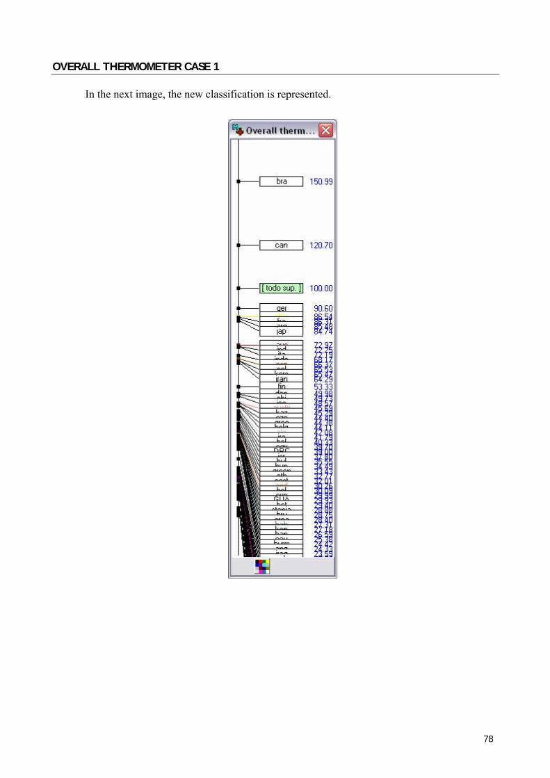
78
OVERALL THERMOMETER CASE 1 In the next image, the new classification is represented.
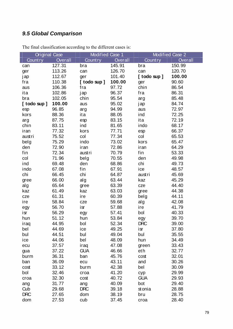
79
9.5 Global Comparison
The final classification according to the different cases is: Original Case Modified Case 1 Modified Case 2
Country Overall Country Overall Country Overall can 127.31 bra 145.91 bra 150.99 ger 113.26 can 126.70 can 120.70 jap 112.67 ger 101.40 [ todo sup ] 100.00 fra 110.38 [ todo sup ] 100.00 ger 90.60 aus 106.36 fra 97.72 chin 86.54 ita 102.86 jap 96.37 fra 86.31 bra 102.05 chin 95.54 arg 85.48 [ todo sup ] 100.00 aus 95.02 jap 84.74 esp 96.85 arg 94.99 aus 72.97 kors 88.36 ita 88.05 ind 72.25 arg 87.75 esp 83.15 ita 72.19 chin 83.11 ind 81.65 indo 68.17 iran 77.32 kors 77.71 esp 66.37 austri 75.52 col 77.34 col 65.53 belg 75.29 indo 73.02 kors 65.47 den 72.90 iran 72.86 iran 64.29 fin 72.34 austri 70.79 fin 53.33 col 71.96 belg 70.55 den 49.98 ind 69.48 den 68.86 chi 49.73 indo 67.08 fin 67.91 ice 48.57 chi 66.45 chi 64.87 austri 45.69 gree 66.00 alg 63.44 kaz 45.29 alg 65.64 gree 63.39 cze 44.40 kaz 61.49 kaz 63.03 gree 44.38 cze 61.31 ire 60.39 belg 44.11 ire 58.84 cze 59.68 alg 42.08 egy 56.70 isr 57.88 ire 41.79 isr 56.29 egy 57.41 bol 40.33 hun 51.12 hun 53.84 egy 39.70 iraq 44.95 bol 52.34 DRC 39.00 bel 44.69 ice 49.25 isr 37.80 bul 44.51 bul 49.04 bul 35.55 ice 44.06 bel 48.09 hun 34.49 ecu 37.57 iraq 47.08 green 33.43 gua 37.22 GUA 46.66 eth 32.77 burm 36.31 ban 45.76 cost 32.01 ban 36.09 ecu 43.11 and 30.26 cost 33.12 burm 42.38 bel 30.09 bol 32.46 croa 41.20 cyp 29.99 croa 32.30 cost 40.72 GUA 29.93 ang 31.77 ang 40.09 bot 29.40 Cub 29.68 DRC 39.18 stonia 28.88 DRC 27.65 dom 38.19 bru 28.75 dom 27.53 cub 37.45 croa 28.40

80
korn 27.42 els 36.25 bah 27.31 ken 27.03 came 35.76 ken 27.18 came 26.79 ken 35.43 ban 26.59 els 25.59 eth 35.19 ecu 25.38 eth 24.37 korn 35.06 burm 24.42 aze 23.39 aze 34.81 ang 24.33 gha 22.76 gha 34.14 iraq 23.59 hon 18.64 green 33.15 cub 18.87 bot 17.67 cyp 32.22 els 14.53 cyp 16.77 bot 31.24 dom 13.39 stonia 14.83 hon 30.79 gab 13.37 cha 14.36 stonia 30.38 korn 11.80 green 14.31 bos 29.41 hon 11.77 bos 13.63 jor 29.25 bos 11.76 cam 13.10 cha 28.42 aze 10.03 jor 13.00 cam 27.75 afg 9.90 Cote 11.44 and 26.81 came 8.39 afg 9.63 bru 25.74 guy 6.29 gui 8.10 Cote 25.36 cha 5.62 and 4.92 gui 25.32 cab 5.23 bru 3.91 bah 24.83 gha 5.06 bah 3.14 afg 23.71 jor 4.74 geo 2.34 geo 21.46 jam 4.68 bur 0.84 gab 19.06 arm 4.33 [ todo inf. ] 0.00 bur 18.89 Cote 3.66 gab -0.39 arm 18.80 alb 3.21 arm -2.44 alb 18.43 geo 2.01 jam -3.64 jam 17.27 EcuGui 1.79 alb -4.00 hai 15.56 car 1.23 hai -6.80 guy 10.70 bur 0.94 guy -12.70 car 8.46 cam 0.23 car -15.65 cab 6.48 [ todo inf. ] 0.00 cab -22.62 ben 5.50 gui -0.23 ben -23.51 EcuGui 3.31 hai -4.57 eri -27.49 eri 1.30 RC -6.01 EcuGui -27.96 [ todo inf. ] 0.00 ben -7.20 RC -34.62 RC -4.14 eri -7.23 gam -42.21 gam -6.10 gam -8.22

81
Chapter 10 - Conclusions M-MACBETH is a software for taking multicriteria decisions. With it, a user can obtain the most adequate alternative according to his/her own preferences.
After the insertion of the criteria, the different options and the judgements defined by the user, M-MACBETH shows the user its results in an easy and clear way with different graphics which, most of them, can be modified to adjust the configuration values.
During the accomplishment of the analysis of this software, the main difficulties we found were:
• Is not possible the loading of options from text files and they must be inputted manually, which in turn results in a loss of time.
• Due to the limitations of this demo version of M-MACBETH, the number of criteria which can be inputted is limited just to four. In the same way, the basis for comparison of the criteria is also limited to qualitative or quantitave performance levels if we establish a high amount of options.
• While M-MACBETH simplifies the arduous task of the expert making easy the carrying out of the calculation of multicriteria decisions with a great amount of alternatives, it requires to setting up of a lot of parameters (judgements, weight of the criteria) for its well development.
On the other side, M-Macbeth has an extended and complete user guide that helps to understand the way to introduce the data and later how to analyse the results obtained.

82
References
BANA E COSTA, C.A.; DE CORTE, J.-M.; VANSNICK, J.-C. “M-MACBETH User Guide
(Version 1.1)”. Included in the M-MACBETH Software. 2005.
FIGUEIRA, J.; GRECO, S.; EHRGOTT, M. “MULTIPLE CRITERIA DECISION ANALYSIS:
State of the Art Surveys”. Springer Science + Business Media, Inc. pp. 409-442. 2005.
http://www.m-macbeth.com/ (31/03/2007)


