Cristina Masoller - fisica.edu.uycris/teaching/slides_masoller_uni.pdf · Discrete Fourier...

Nonlinear time series analysis:Univariate analysis

Cristina MasollerUniversitat Politecnica de Catalunya, Terrassa, Barcelona, Spain

[email protected]

www.fisica.edu.uy/~cris

Introduction

− Historical developments: from dynamical systems to complex systems

Univariate analysis

− Methods to extract information from a time series.

− Applications.

Bivariate analysis

− Extracting information from two time series.

− Correlation, directionality and causality.

− Applications.

Multivariate analysis

‒ Many time series: complex networks.

‒ Network characterization and analysis.

‒ Applications.

Outline

2

Return maps

Correlation and Fourier analysis

Stochastic models and surrogates

Distribution of data values

Attractor reconstruction: Lyapunov exponents and fractal

dimensions

Symbolic methods

Information theory measures: entropy and complexity

Network representation of a time-series

Spatio-temporal representation of a time-series

Instantaneous phase and amplitude

Methods of time-series analysis

3

X = {x1, x2, … xN}

First step: Look at the data.

Examine simple properties:

‒ Return map: plot of xi vs. xi+

‒ Distribution of data values

‒ Auto-correlation

‒ Fourier spectrum

To begin with the analysis of a time-series

4

Bi-decadal oxygen isotope data set d18O (proxy for

palaeotemperature) from Greenland Ice Sheet Project

Two (GISP2) for the last 10,000 years with 500 values

given at 20 year intervals.

First example of a geophysical time series

5A. Witt and B. D. Malamud, Surv Geophys (2013) 34:541–651

Discharge of the Elkhorn river (at Waterloo, Nebraska,

USA) sampled daily for the period from 01 January

1929 to 30 December 2001.

Second example


The geomagnetic auroral electrojet (AE) index sampled

per minute for the 24 h period of 01 February 1978 and

the differenced index:

Third example


Calculate the return maps and the distribution of data

values for different values of the control parameter, r[3,4],

starting from a random initial condition, x(1) (0,1).

Which is the influence of dynamical or observational noise?

Exercise 1a: The Logistic map

8

)](1)[( )1( ixixrix

r=3.9, no noise

Observational noise

(D=0.01)

9

Dynamical noise

(D=0.01)

The return maps reveal different degrees of

correlations between consecutive data values.

How to quantify?

Linear tool: the autocorrelation function

For a stationary process (such that the mean

value and are time-independent):

Autocorrelation function (ACF)

10

)()(

2

Cxxxx

Ctt

Autocorrelation:

Quantifies persistence (memory)

11

Persistence: large values tend to follow large ones, and

small values tend to follow small ones.

Anti-persistence: large values tend to follow small ones

and small values large ones.

Short-range correlations: values are correlated with one

another at short lags in time

Long-range correlations: values are correlated with one

another at very long lags in time (all or almost all values are

correlated with one another)

Back to the three examples of geophysical time series


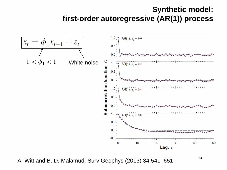
Synthetic model:

first-order autoregressive (AR(1)) process

13

White noise

A. Witt and B. D. Malamud, Surv Geophys (2013) 34:541–651

Calculate the autocorrelation function of the Logistic

time series generated in Ex. 1a.

Can they be fit by an AR(1) process?

Exercise 1b

14

Describes a signal in terms of its oscillatory components.

Example: climatic time series involve oscillations in a wide

range of scales

‒ hours to days,

‒ months to seasons,

‒ decades to centuries,

‒ and even longer...

Fourier analysis

An ‘‘artist’s

representation’’ of the

power spectrum of

climate variability (Ghil

2002).

Odd-order harmonics

Fourier analysis describes a signal in terms of its

oscillatory components

16

Even-order harmonics?

Mammals use the Fourier Transformation for hearing

Source: Richard Alan Peters II, Vanderbilt University

Fourier is linear but in nonlinear systems, “Ghost resonance”:

Response of a model neuron, driven simultaneously by noise and at

least two weak signals with frequencies components k f0 , (k+1) f0 , . . .

(k+n) f0with k>1. Depending on the noise, the neuron’s pulses are

spaced by 1/f0, i.e., it “hears” a frequency that is missing in the input.

Chialvo et al, PRE 65, 050902R (2002)

Discrete Fourier Transform

= sampling interval

Xk = complex Fourier coeff. associated to freq. fk= k/(N)

The PSD indicates the intensity of each frequency component:

How to calculate? Fast Fourier Transform (FFT). N=2m.

With Matlab: z=fft(x); q=z.*conj(z); v=ifft(q).

For stationary signals the inverse FT of the PSD is |C()|

(Wiener–Khinchin theorem). Further reading:

Press WH et al. Numerical recipes in C/Fortran: the art of scientific computing

(Cambridge University Press)

The Power Spectrum (or power spectral density, PSD)

18

Check that the inverse FT of the PSD is the |ACF|, |C()|,

using AR(1) and logistic-map time series.

Exercise 2: PSD and ACF

19

AR(1), 1=0.8 AR(1), 1= -0.5 Logistic, r=3.9

|C()| and IFFT(PSD)

x=x(1:ndats);

x=x-mean(x);

z=fft(x);

psd=z.*conj(z);

s=ifft(psd);

v=sqrt(s.*conj(s));

ctau=v/max(v);

Discrete Fourier transform

is designed for ‘circular’ time series (i.e. the last and first

values in the time series ‘follow’ one another).

Large values of xN-x1 (typical in non-stationary time series)

can result in spurious artifacts.

It is recommended to normalize to =0, =1 and to remove

the trend (“detrend”) before computing the FFT.

Simple ways to detrend:

− Take the best-fit straight line to the time series and

subtract it from all the values.

− Connect a line from the first point to the last point and

subtract this line from the time series, forcing xN=x1=0

Numerical technicalities

20

In short time series pre-processing reduces the

impact of the initial and final data points

21

Choose a “weight shape” and multiply each value of

the time series by its weight.


Example: El Niño 3.4 index

Sea surface temperature (SST) anomaly in the Eastern

tropical Pacific Ocean

22

Year resolution, Source: climate explorer

From 5°N to 5°S and from 170°W to 120°W

An El Niño (La Niña) event is identified if the 5-month running-

average of the NINO3.4 index exceeds +0.4°C (-0.4°C) for at

least 6 consecutive months.

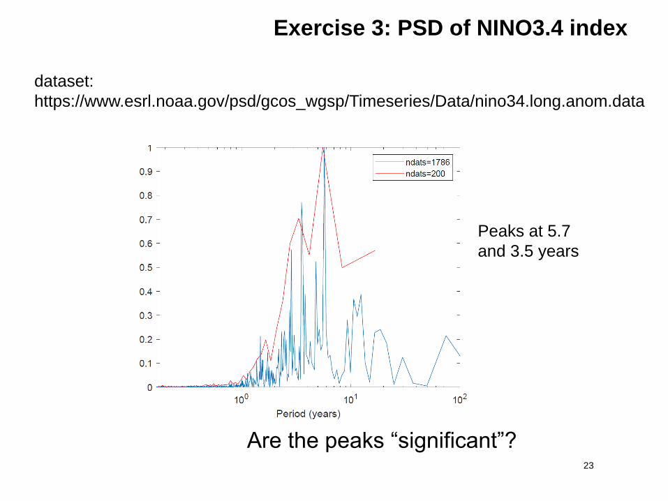
Exercise 3: PSD of NINO3.4 index

23

Are the peaks “significant”?

dataset:

https://www.esrl.noaa.gov/psd/gcos_wgsp/Timeseries/Data/nino34.long.anom.data

Peaks at 5.7

and 3.5 years

Real observed time series.

Generate an ensemble of

“surrogate” time series that are

both “similar“ to the original and

also consistent with the specific

null hypothesis (NH) that we

want to test.

Measure an statistical property:

“d” in the original series and “s(i)”

in the ensemble time series.

Is “d” consistent with the

distribution of “s(i)” values?

− No! we reject the NH.

− Yes! we “fail to reject” the NH.

The method of surrogate data

Taken from

M. Small, Applied Nonlinear Time

Series Analysis (World Scientific,

2005)

Source: wikipedia

p value

25

The p-value only measures the compatibility of an observation

with a hypothesis, not the truth of the hypothesis.

Altman, N. and Krzywinski, M. Interpreting P values. Nature Methods 14, 213 (2017).

Example

26

Red: MI and DI values computed from original data

Histogram: MI and DI values computed from surrogates

Think lines: significance thresholds (mean +/- 3 )

In both cases the NH (no MI, no DI) is rejected.

Further reading: G. Lancaster et al, “Surrogate data for hypothesis

testing of physical systems”, Physics Reports 748 (2018) 1–60.

Surrogate test for nonlinearity

27

A: Rossler with

a = 0.165, b = 0.2

and c = 10

B: High-order (linear) autoregressive process

Proper surrogates detect nonlinearity in

A (reject NH) but not in B (fail to reject NH)

Return maps





dimensions

Symbolic methods






28

Mean (expected value of X): =)

Variance: 2 =Var (X) = E[(X-)2]

Skewness: “measures” the asymmetry of the distribution

Kurtosis: measures the "tailedness“ of the distribution. For a

normal distribution K=3.

Coefficient of variation: normalized measure of the width of

the distribution. Cv = / ||

How to characterize the

distribution of data values?

29

S = E[Z3]

K = E[Z4]

30

Source: Numerical Recipes

Comparison of probability distributions

31


32


How to “bin” data (linear vs. logarithmic bins, how to chose the

size of the bins)

Number of data points in each bin (minimum average 10)

How to fit the distribution (assuming a statistical model, the

maximum likelihood estimator selects the parameter values

which give the observed data the largest probability).

Is the fit appropriated for the data? Many goodness of fit tests.

Challenges in the analysis of the distribution of data values

33

Can different regimes be identified? With what reliability?Time

Low current (noise?)

High current (chaos?)

Example: intensity emitted by a diode laser with feedback,

as the pump current increases

Intermediate: spikes

Time

Time

Standard deviation of the intensity time series, σ,

recorded using three different sampling rates

35C. Quintero-Quiroz et al, Scientific Reports (2016)

Laser pump current, normalized to the threshold value

http://www.nature.com/articles/srep37510

36

If the skewness and

kurtosis of the distribution

of values are “consistent”

with a Gaussian → noise

Else, if increases with the

pump current → spikes

Else → chaos

Classification criteria

Panozzo et al, Chaos 27, 114315 (2017)

spikes

noise

chaos

I = {i1, i2, … iN} laser “raw” intensity recorded for

different pump currents and feedback strengths

http://aip.scitation.org/doi/abs/10.1063/1.4986441?ai=1gvoi&mi=3ricys&af=R

Threshold crossing ``events’’

Ti = ti+1 - tiinter-spike-intervals (ISIs):

Problems:

‒ How to select

the threshold?

‒ Threshold

dependent

results?

From time series to sequence of events

“Features” that

persist for a

wide range of

thresholds are

"true" features.

Example: by counting the number of times

the laser intensity falls below a threshold

we can (almost) distinguish three regimes.

38Panozzo et al, Chaos 27, 114315 (2017)

spikes

noise

chaos

-1.5


Exercise 4a: calculate PSD of the laser intensity time series.

Calculate the number of events as a function of the threshold.

Compare with El Niño time series.

39

http://www.fisica.edu.uy/~cris/datasets/lff.dat

Exercise 5: repeat the analysis for the time

series of the intensity of a fiber laser

40

Stochastic and coherence

resonances

Bistable system with sinusoidal forcing and noise

42

Varying ; D constant

Time

Varying D; constant

D

Time

x(t)

Gammaitoni et al, Rev. Mod. Phys. 70, 223 (1998)

Quantification of stochastic resonance with spectral analysis

43

Phase-averaged power spectral

density: average over many

realizations of the noise and average

over the input initial phase .

Signal to noise ratio at

SNR()=

Noise strength, D


Quantification of stochastic resonance

with the distribution of residence times


44

Strength of the nth peak: area under the peak

Number of

switching

times

D

Neuron model: Fitz Hugh–Nagumo

(=0.01, a =1.05)

Coherence resonance

45

Autocorrelation

Pikovsky and Kurths, Phys. Rev. Lett. 78, 775 (1997)

D

Characteristic correlation time

Coefficient of variation of inter-spike-interval distribution Cv=/

How to quantify coherence resonance?

46

c solid

Cv dashed

Pikovsky and Kurths, Phys. Rev. Lett. 78, 775 (1997)

LockingThe frequency of an oscillator is

controlled by an external signal

Experimental data: the laser pump current is

modulated with a small-amplitude sinusoidal signal

48

Laser

output

Input

signal

fmod = 14 MHz 30 MHz 50 MHz

Tiana et al, Opt. Express 26, 323041 (2018)

https://www.osapublishing.org/oe/abstract.cfm?uri=oe-26-7-9298&origin=search

How does the distribution of inter-spike intervals look like?

49Tiana et al, arXiv:1806.08950v1 (2018)

https://arxiv.org/abs/1806.08950

Coefficient of variation of the ISI distribution Cv=/

How to quantify the degree of locking?

50

Laser current

[mA]

increases the

frequency of the

“natural” spikes

Tiana et al, Opt. Express 26, 323041 (2018)

https://www.osapublishing.org/oe/abstract.cfm?uri=oe-26-7-9298&origin=search

Chaos

Return maps





dimensions

Symbolic methods






52

Attractor reconstruction: “embed” the time series in a phase-space

of dimension d using delay coordinates

53

Adapted from U. Parlitz (Gottingen)

How to identify (and quantify) chaos in observed data?

Observed time series S = {s(1), s(2), … s(t) … }

Reconstruction using delay coordinates

54

A problem: how to chose the embedding parameters

(lag , dimension d)

Bradley and Kantz, CHAOS 25, 097610 (2015)

is chosen to maximize the spread of the data in phase

space: the first zero of the autocorrelation function (or where

|C()| is minimum)

d is often estimated with the false nearest neighbors

technique that examines how close points in phase space

remain close as the dimension is increased.

Points that do not remain close are ‘false’ neighbors.

The number of false neighbors decreases as the embedding

dimension is increased.

The first dimension for which the number of false neighbors

decreases below a threshold provides the estimated d.

How to chose the lag and the dimension d

55

After reconstructing the attractor, we can characterize the

TS by the fractal dimension and the Lyapunov exponent.

A stable fixed point has negative s (since perturbations

in any direction die out)

An attracting limit cycle has one zero and negative s

A chaotic attractor as at least one positive .

56

Adapted from U. Parlitz

Lyapunov exponents: measure how

fast neighboring trajectories diverge

Initial distance

Final distance

Local exponential grow

The rate of grow is averaged over the attractor,

which gives max

Steps to compute the maximum LE

57

A very popular method for detecting

chaos in experimental time series.

A word of warning!

58

The rate of grow depends on the direction in the phase space.

The algorithm returns in the fastest expansion direction.

Therefore, the algorithm always returns a positive number!

This is a problem when computing the LE of noisy data.

First we need to test nonlinearity in the time series.

Further reading: − F. Mitschke and M. Damming, Chaos vs. noise in

experimental data, Int. J. Bif. Chaos 3, 693 (1993)

− A. Pikovsky and A. Politi, Lyapunov Exponents (Cambridge

University Press, 2016)

Example: the fractal dimension of a coastline quantifies how

the number of scaled measuring sticks required to measure

the coastline changes with the scale applied to the stick.

Fractal dimension

59

Fractal dimension:

Source: wikipedia

→

Another very popular method for detecting chaos

in real-world data.

Grassberger-Procaccia correlation dimension algorithm

60

Further reading:

P. Grassberger and I. Procaccia, "Measuring the Strangeness of Strange Attractors".

Physica D vol. 9, pp.189, 1983.

L. S. Liebovitch and T. Toth, “A fast algorithm to determine fractal dimensions by

box counting,” Physics Letters A, vol. 141, pp. 386, 1989.

Fractal dimension (box counting dimension):

Problem: for time-series analysis, no distinction between

frequent and unfrequently visited boxes.

An alternative: the

correlation dimension.

g is the number of pairs of

points with distance

between them < .

Example of application of fractal analysis:

distinguishes between diabetic retinopathy and normal patients

61

Source: Pablo Amil, UPC

→

The fractal dimension of the blood vessels − in the normal human retina is 1.7

− tends to increase with the level of diabetic retinopathy

− varies considerably depending on the image quality and the technique

used for measuring the fractal dimension

Symbolic methods to identify patterns

and structure in time series

62

Laser spikes

Time (s)

63

Can lasers mimic real neurons?

Time (ms)

Neuronal spikes

A. Longtin et al PRL (1991)

Experimental data when the laser

current is modulated with a

sinusoidal signal of period T0.

2T0 4T0

A. Aragoneses et al

Optics Express (2014)64

Are there statistical similarities between neuronal

spikes and optical spikes?

http://www.opticsinfobase.org/oe/viewmedia.cfm?URI=oe-22-4-4705&seq=0&origin=search


A. Longtin

Int. J. Bif. Chaos (1993)

Laser ISIsNeuronal ISIs

M. Giudici et al PRE (1997)

A. Aragoneses et al

Optics Express (2014)

Return maps of inter-spike-intervals

Ti

Ti+1

65

HOW TO INDENTIFY TEMPORAL ORDER?

MORE/LESS EXPRESSED PATTERNS?



The time series {x1, x2, x3, …} is transformed (using an

appropriated rule) into a sequence of symbols {s1, s2, …}

taken from an “alphabet” of possible symbols {a1, a2, …}.

Then consider “blocks” of D symbols (“patterns” or “words”).

All the possible words form the “dictionary”.

Then analyze the “language” of the sequence of words

- the probabilities of the words,

- missing/forbidden words,

- transition probabilities,

- information measures (entropy, etc).

Symbolic analysis

66

if xi > xth si = 0; else si =1

transforms a time series into a sequence of 0s and 1s, e.g.,

{011100001011111…}

Considering “blocks” of D letters gives the sequence of

words. Example, with D=3:

{011 100 001 011 111 …}

The number of words (patterns) grows as 2D

More thresholds allow for more letters in the “alphabet”

(and more words in the dictionary). Example:

if xi > xth1 si = 0;

else if xi < xth2 si =2;

else (xth2 <x i < xth1) si =1.

Threshold transformation: “partition” of the phase space

67

Ordinal rule: if xi > xi-1 si = 0; else si =1

also transforms a time-series into a sequence of 0s and 1s

without using a threshold

“words” of D letters are formed by considering the order

relation between sets of D values {…xi, xi+1, xi+2, …}.

D=3

Alternative rule

68Bandt and Pompe PRL 88, 174102 (2002)

https://journals.aps.org/prl/abstract/10.1103/PhysRevLett.88.174102

021 012

Relative order of three consecutive intervals

{…Ii, Ii+1, Ii+2, …}

Example: (5, 1, 7) gives “102” because 1 < 5 < 7

Ordinal

probabilities

1 2 3 4 5 6

Ii = ti+1 - ti

The number of ordinal patterns increases as D!

A problem for short datasets

How to select optimal D?

it depends on:

─ The length of the data

─ The length of the correlations

Threshold transformation:

if xi > xth si = 0; else si =1

Advantage: keeps information

about the magnitude of the

values.

Drawback: how to select an

adequate threshold (“partition”

of the phase space).

2D

Ordinal transformation:

if xi > xi-1 si = 0; else si =1

Advantage: no need of

threshold; keeps information

about the temporal order in

the sequence of values

Drawback: no information

about the actual data values

D!

71

Comparison

2 4 6 8 1010

0

102

104

106

108

D

2D

D!

Number

of

symbols

Null hypothesis:

pi = p = 1/D! for all i = 1 … D!

If at least one probability is not in the

interval p 3 with

and N the number of ordinal patterns:

We reject the NH with 99.74%

confidence level.

Else

We fail to reject the NH with

99.74% confidence level.

Are the D! ordinal patterns equally probable?

72

Npp /)1(

Logistic map

1 2 3 4 5 60

50

100

150

200

0 0.2 0.4 0.6 0.8 10

10

20

30

40

50

0 100 200 300 400 500 6000

0.2

0.4

0.6

0.8

1

550 555 560 565 570 575 580 585 590 595 6000

0.2

0.4

0.6

0.8

1

Time series Detail

Histogram D=3 Patterns Histogram x(t)

forbidden

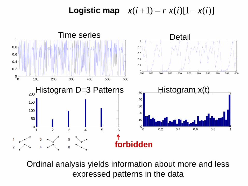
Ordinal analysis yields information about more and less

expressed patterns in the data

)](1)[( )1( ixixrix

Deterministic systems (such as the logistic map) can

have forbidden patterns, while stochastic systems

have missing patterns (unobserved patterns due to

the finite length of the time series).

Forbidden or missing patterns?

74

Number of missing D=3 patterns found in 1000 time series generated with the logistic map (r=4), as a function of the length of the series.

M. Zanin et al, Entropy 14, 1553 (2012)

210

It can provide a way to quantify the degree of stochasticity.

Can this be useful for distinguishing noise from chaos?

75

Less stochastic

J. Tiana-Alsina et al, Phil. Trans. Royal Soc. A 368, 367 (2010)

# m

issin

g p

attern

s

Example:

experimental data is

transformed into a

sequence of 0s and

1s, the patterns are

formed by 8

symbols; the

number of possible

patterns is 28 = 256.

Ordinal analysis identifies the onset of different dynamical

regimes, but fails to distinguish “noise” and “chaos”

C. Quintero-Quiroz et al, Scientific Reports (2016)

A probability value in the gray region is consistent

with p= 1/6 0.17 with 99.7% confidence level.

0.14

0.17

0.24

Laser pump current, normalized to the threshold value

http://www.nature.com/articles/srep37510

Another way to (almost) “classify” the laser intensity

time series into noise, spikes or chaos

77Panozzo et al, Chaos 27, 114315 (2017)

spikes

noise

chaos

P(210)

210

Gray region: P(210) is consistent with 1/6 with 3 confidence level.


Gaussian white noise and

subthreshold signal: a0 and T such

that spikes are noise-induced.

Time series with M=100,000 ISIs

simulated (a=1.05, =0.01).

Gray region: significance analysis

with 3 confidence level.

J. M. Aparicio-Reinoso et al PRE 94, 032218 (2016)

Example: neuron model

T=20

D=0.015

Fitz Hugh–Nagumo model

http://journals.aps.org/pre/abstract/10.1103/PhysRevE.94.032218

Data requirements: influence of the number of patterns

79J. M. Aparicio-Reinoso et al PRE 94, 032218 (2016)

With external signal

Without external signal


Side note: comparison with the laser spikes

Modulation amplitudeModulation amplitudeA. Aragoneses et al, Sci. Rep. 4, 4696 (2014)J. M. Aparicio-Reinoso et al PRE 94, 032218 (2016)

http://www.nature.com/srep/2014/140415/srep04696/full/srep04696.html


Role of the period of the external signal

Signal Period Signal Period


Weak noise Stronger noise


Ordinal (nonlinear) analysis vs. linear correlation analysis

82

For strong noise, the auto-correlation at lags 1 and 2 vanish but

ordinal analysis detects patterns with different probabilities.

M. Masoliver and C. Masoller, Scientific Reports 8, 8276 (2018).

Detecting longer correlations

Example: climatological data (monthly sampled)

− Consecutive months:

− Consecutive years:

Varying = varying temporal resolution (sampling time)

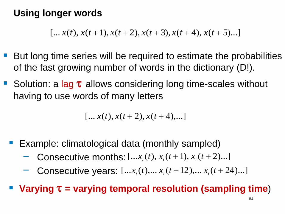
Using longer words

)...]24( ),...12( ),...([... txtxtx iii

)...]2( ),1( ),([... txtxtx iii

Solution: a lag allows considering long time-scales without

having to use words of many letters

84

)...]5( ),4(),3(),2(),1( ),( [... txtxtxtxtxtx

),...]4(),2(),( [... txtxtx

But long time series will be required to estimate the probabilities

of the fast growing number of words in the dictionary (D!).

Ordinal patterns can be defined using a lag time between

the data points (varying the effective “sampling time”)

Example: el Niño index, monthly sampled‒ Green

triangles:

intra-

seasonal

pattern,

‒ blue

squares:

intra-annual

pattern

‒ red circles:

inter-annual

pattern

Example of application of ordinal

analysis to ECG-signals

86

Time series of inter-beat intervals

congestive

heart failure

healthy

subject

Classifying ECG-signals according

to the frequency of words

87

(the probabilities are normalized with respect to the

smallest and the largest value occurring in the data set)

U. Parlitz et al. Computers in Biology and Medicine 42, 319 (2012)

http://www.fisica.edu.uy/~cris/Parlitz_2012.pdf

Software

88

Python and Matlab codes for computing

the ordinal pattern index are available

here: U. Parlitz et al. Computers in

Biology and Medicine 42, 319 (2012)

World length (wl): 4

Lag = 3 (skip 2 points)

Result:

indcs=3

http://www.fisica.edu.uy/~cris/Parlitz_2012.pdf

3.5 3.55 3.6 3.65 3.7 3.75 3.8 3.85 3.9 3.950

0.1

0.2

0.3

0.4

0.5

0.6

0.7

0.8

0.9

Normal bifurcation diagram Ordinal bifurcation diagram

Exercise 6: compute the “ordinal” bifurcation diagram of

the Logistic map with D=3.

Xi

Map parameter Map parameter, r

Pattern 210 is always forbidden;

pattern 012 is more frequently

expressed as r increases

Ordinal

Probabilities

012 021 102 120 201 210

Calculate the probabilities of the D=2 and 3 ordinal patterns

for the diode laser intensity time-series. How do they depend

on the lag? Compare with the time series of NINO3.4 index.

Exercise 7a: ordinal probabilities vs lag.

90

NINO3.4 indexDiode laser intensity

Exercise 7b: repeat the analysis for the fiber laser intensity

91

Pump power 0.9 W Pump power 1.5 W

A. Aragoneses et al, Phys. Rev. Lett. 116, 033902 (2016).

L. Carpi and C. Masoller, Phys. Rev. A 97, 023842 (2018).

How to quantify unpredictability

and complexity?

Return maps





dimensions

Symbolic methods






93

The time-series is described by a set of probabilities

Shannon entropy:

Interpretation: “quantity of surprise one should feel upon

reading the result of a measurement” K. Hlavackova-Schindler et al, Physics Reports 441 (2007)

Simple example: a random variable takes values 0 or 1 with

probabilities: p(0) = p, p(1) = 1 − p.

H = −p log2(p) − (1 − p) log2(1 − p).

p=0.5: Maximum unpredictability.

Information measure: Shannon entropy

i

ii ppH 2log

11

N

i

ip

940 0.5 10

0.2

0.4

0.6

0.8

1

p

HShannon entropy computed from ordinal

probabilities: Permutation Entropy

Permutation entropy (PE) of the Logistic map

Bandt and Pompe

Phys. Rev. Lett. 2002

95

Entropy per symbol:

x(i+1)=r x(i)[1-x(i)]

Robust to noise

Entropy: measures unpredictability or disorder.

How to quantify Complexity?

H = 0

C = 0

H ≠ 0

C ≠ 0

H = 1

C = 0

Order DisorderChaos

We would like to find a quantity “C” that measures complexity,

as the entropy, “H”, measures unpredictability, and, for low-

dimensional systems, the Lyapunov exponent measures chaos.

Source: O. A. Rosso

Feldman, McTague and Crutchfield, Chaos 2008

“A useful complexity measure needs to do more

than satisfy the boundary conditions of vanishing

in the high- and low-entropy limits.”

“Maximum complexity occurs in the region

between the system’s perfectly ordered state

and the perfectly disordered one.”

i

iiS ppPSPI ln][][

i

q

i

q

T pq

PSPI 11

1][][

i

q

i

q

R pq

PSPI ln1

1][

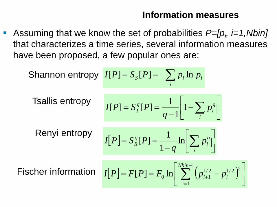
Information measures

Assuming that we know the set of probabilities P=[pi, i=1,Nbin]

that characterizes a time series, several information measures

have been proposed, a few popular ones are:

Shannon entropy

Tsallis entropy

Renyi entropy

1

1

22/12/1

10 ln][Nbin

i

ii ppFPFPIFischer information

max

][][

I

PIPH

where and Pe is the equilibrium probability

distribution (that maximizes the information measure).

Example: if I[P] = Shannon entropy

then Pe = [pi=1/Nbin for i=1,Nbin]

and Imax = ln(Nbin)

][max ePII

1][0 PH

Normalization

Measures the “distance“ from P to the equilibrium

distribution, Pe

where Qo is a normalization constant such that 1][0 PQ

ePPDQPQ ,][ 0

Disequilibrium Q

i

eiiEeeE ppPPPPD2

,],[

PIPIPPKPPD eeeK ][],[

2

],[PPKPPK

PPDee

eJ

Distance between two probability distributions P and Pe

Read more: S-H Cha: Comprehensive Survey on Distance/Similarity Measures

between Probability Density Functions, Int. J of. Math. Models and Meth. 1, 300 (2007)

Euclidean

Kullback

Jensen divergence

A family of complexity measures

can be defined as:

where

A = S, T, R (Shannon, Tsallis, Renyi)

B = E, K, J (Euclidean, Kullback, Jensen)

][][][ PQPHPC BA

][][][ PQPHPC JSMPR

][][][ PQPHPC ESLMC Lopez-Ruiz, Mancini & Calbet, Phys. Lett. A (1995).

Anteneodo & Plastino, Phys. Lett. A (1996).

Martín, Plastino & Rosso, Phys. Lett. A (2003).

Statistical complexity measure C

The complexity of the Logistic Map

103

x(i+1)=r x(i)[1-x(i)]

Martín, Plastino, & Rosso, Physica A 2006

Euclidian

distance

Jensen

distance

Map parameter

Map parameter

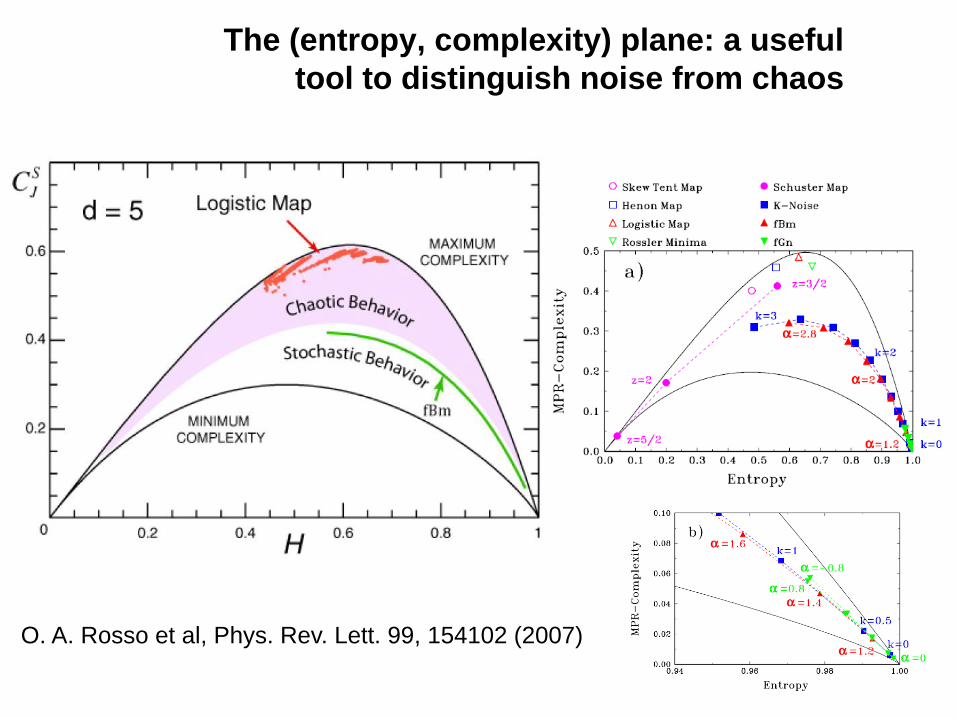
The (entropy, complexity) plane: a useful

tool to distinguish noise from chaos

104

O. A. Rosso et al, Phys. Rev. Lett. 99, 154102 (2007)

Many complexity measures have been proposed

105

Further reading: L. Tang et al, “Complexity testing techniques for time series data: A

comprehensive literature review”, Chaos, Solitons and Fractals 81 (2015) 117–135

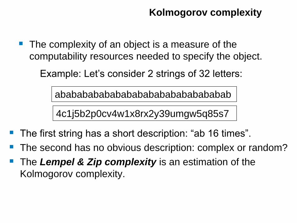
The complexity of an object is a measure of the

computability resources needed to specify the object.

Kolmogorov complexity

Example: Let’s consider 2 strings of 32 letters:

abababababababababababababababab

4c1j5b2p0cv4w1x8rx2y39umgw5q85s7

The first string has a short description: “ab 16 times”.

The second has no obvious description: complex or random?

The Lempel & Zip complexity is an estimation of the

Kolmogorov complexity.

Lempel & Zip complexity of

the Logistic Map

107Kaspar and Schuster, Phys Rev. A 1987

Exercise 7c: compute the PE vs. lag for the diode

laser intensity time series and NINO3.4 index

108

Laser intensity NINO3.4 index

How to quantify

- the degree of unpredictability of Surface Air Temperature

(SAT) anomaly, and

- the degree of nonlinear response of SAT to solar forcing?

Proposed measures

- Shannon entropy of SAT anomaly distribution of values (no

symbols)

- Distance from SAT to insolation (incoming solar radiation)

Example of application to climate data

109

Monthly mean SAT from two reanalysis (NCEP CDAS116

and ERA Interim17). The spatial resolution is 2.5°/1.5° and

cover the time-period [1949–2015]/[1980–2014] respectively.

− NCEP CDAS1: N =10224 time series of length L = 792

− ERA Interim: N = 28562 and L = 408.

Freely available.

Reanalysis = run a sophisticated model of general

atmospheric circulation and feed it with the available

experimental data, in the different points of the Earth, at their

corresponding times (data assimilation).

This restricts the solution of the model to one as close to

reality as possible in regions where data is available, and to

a solution physically “plausible” elsewhere.

Data

110

Raw SAT, climatology and insolation

111

Climatology:

Monthly data,

Y number of years

Nonlinear response: distance between climatology and

insolation

112

di when i minimizes didi when i = 0

x (insolation) and y (climatology) are both normalized to =0 and =1

i values (months)

F. Arizmendi, M. Barreiro and C. Masoller, “Identifying large-scale patterns

of unpredictability and response to insolation in atmospheric data”,

Sci. Rep. 7, 45676 (2017).

http://rdcu.be/qwUE

http://rdcu.be/qwUE

Unpredictability of SAT anomaly

113

Shannon Entropy: SAT anomaly is normalized to =0 and =1

NCEP CDAS1 ERA Interim

F. Arizmendi, M. Barreiro and C. Masoller, Sci. Rep. 7, 45676 (2017)

Differences are due to the presence of extreme values

in one re-analysis but not in the other.

http://rdcu.be/qwUE

Return maps





dimensions

Symbolic methods






114

A graph: a set of

“nodes” connected

by a set of “links”

Nodes and links can

be weighted or

unweighted

Links can be

directed or

undirected

More in part 3

(multivariate time

series analysis)

What is a network?

We use symbolic patterns as the nodes of the network.

And the links? Defined as the transition probability →

Adapted from M. Small (The University of Western Australia)

In each node i:

j wij=1

Weigh of node i: the

probability of pattern i

(i pi=1)

Weighted and

directed network

Network-based diagnostic tools

• Entropy computed from node weights (permutation entropy)

• Average node entropy (entropy of the link weights)

• Asymmetry coefficient: normalized difference of transition

probabilities, P(‘01’→ ‘10’) - P(‘10’→ ’01’), etc.

iip pps log

(0 in a fully symmetric network;

1 in a fully directed network)

ijiji wws log

A first test with the

Logistic map

D=4

Detects the merging

of four branches, not

detected by the

Lyapunov exponent.

C. Masoller et al, NJP (2015)

Sp = PE

Sn=S(TPs)

Lyapunov

exponent

Map parameter

Slinks

ac

http://iopscience.iop.org/1367-2630/17/2/023068/pdf/1367-2630_17_2_023068.pdf

Approaching a “tipping point”

119

Control parameter

Can we use the ordinal network method to detect

an early warning signal of a critical transition?

Approach to a bifurcation point → eigenvalue with 0 real part

→ long recovery time of perturbations

Critical Slowing Down: increase of autocorrelation and variance

Early warning indicators

Apply the ordinal network method to laser data

Two sets of experiments: intensity time series were recorded

‒ keeping constant the laser current.

‒ while increasing the laser current.

We analyzed the polarization that turns on / turns off.

Is it possible to anticipate the switching?

No if the switching is fully stochastic.

As the laser current increases

Time

Intensity @ constant current

Time

Early warning

Deterministic mechanisms

must be involved.

First set of experiments (the current is kept constant):

despite of the stochasticity of the time-series, the node

entropy “anticipates” the switching


Laser current

I

Laser current

I

Laser current

Node

entropy

sn

(D=3)

No

warning

L=1000

100 windows


The warning is robust with respect to the length

of the pattern D and the length of the window L

Node

entropy

50001000L=500

D=3

Laser current

Laser current

L=1000

D=2 D=3 D=4

Node

entropy



In the second set of experiments (current increases

linearly in time): an early warning is also detected

Node

entropy

Time

With slightly

different

experimental

conditions: no

switching.


L=500, D=3

1000 time series

Time


Second application of the ordinal network method:

distinguishing eyes closed and eyes open brain states

Analysis of two EEG datasets

BitBrain PhysioNet

Eye closed Eye open

Symbolic analysis is applied to the raw data; similar

results were found with filtered data using independent

component analysis.

“Randomization”: the entropies increase and the

asymmetry coefficient decreases

Time window = 1 s

(160 data points)

C. Quintero-Quiroz et al, “Differentiating resting brain states using ordinal

symbolic analysis”, Chaos 28, 106307 (2018).


Another way to represent a time series as a

network: the horizontal visibility graph (HVG)

Luque et al PRE (2009); Gomez Ravetti et al, PLoS ONE (2014)

Unweighted and undirected graph

Rule: data points i and j are connected if there is “visibility”

between them

i

Xi

Parameter free!

Consider the following time series:

Exercise

129

How many links does each data point have?

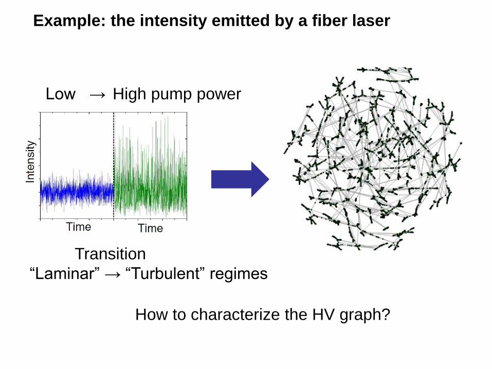
Example: the intensity emitted by a fiber laser

How to characterize the HV graph?

Low → High pump power

Transition

“Laminar” → “Turbulent” regimes

The degree distribution: usual way to characterize a graph

Strogatz, Nature 2001

RegularRandom Scale-free

Surrogate

HVG or PE

“Thresholded” data

S

Different ways of calculating the entropy S uncover

gradual or sharp Laminar → Turbulence transition

Aragoneses et al, PRL (2016)

“Raw” data

(the abrupt transition is robust with

respect to the selection of the threshold)

HVG

PE

S

Time

2


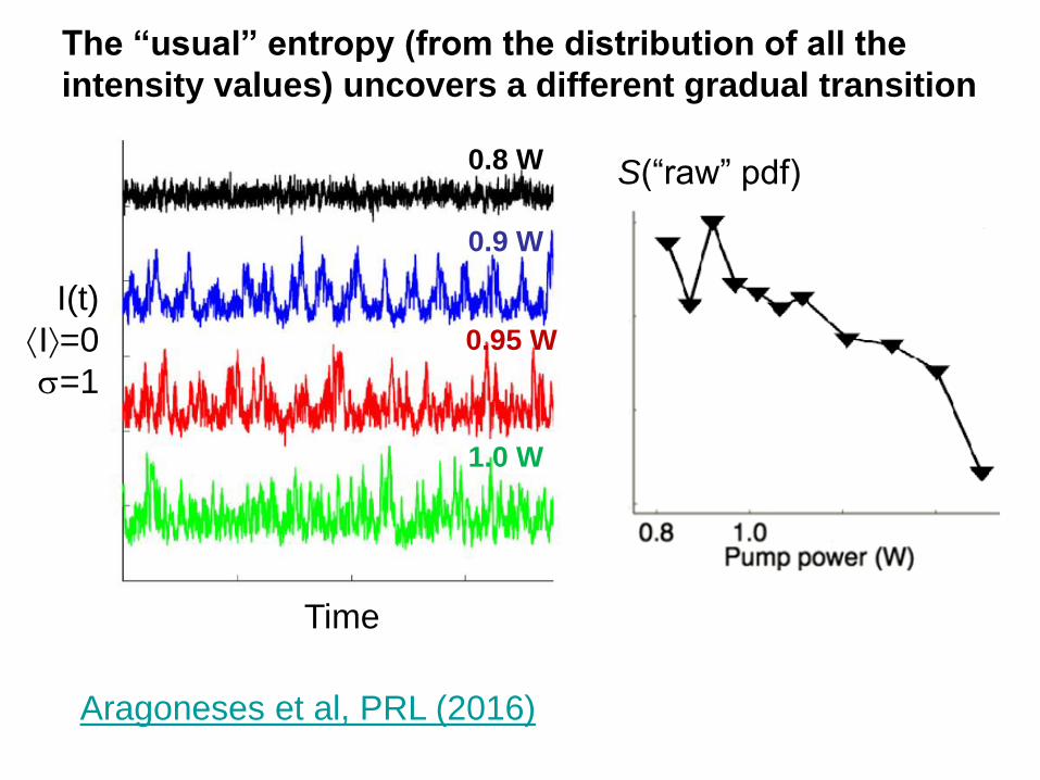
The “usual” entropy (from the distribution of all the

intensity values) uncovers a different gradual transition


I(t)

I=0

=1

0.8 W

1.0 W

0.9 W

0.95 W

Time

S(“raw” pdf)


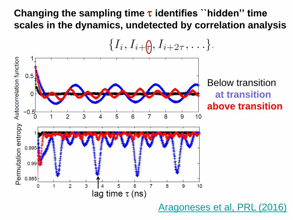
Changing the sampling time identifies ``hidden’’ time

scales in the dynamics, undetected by correlation analysis

Below transition

at transition

above transition



Space-time representation of

a time series

The space-time representation of the intensity time series:

a convenient way to visualize the dynamics

Color

scale: Ii

III

III

III

...

...

...

............

21

221

32212{I1, I2, … I , I+1 ,…}

n

→

=396 dt 431dt

n

496dt



The space time representation: a “visual” tool for

characterizing dynamical variations.

137C. Masoller, Chaos 7, 455-462 (1997).

Embed the time series (find the embedding dimension and lag)

Construct a binary matrix: Aij=1 if xi and xj are “close”, else Aij=0

Plot Aij

Recurrence plots: another way to “visualize” a time series

138

Further reading: R.V. Donner, M. Small, et al. “Recurrence-based time series analysis

by means of complex network methods”, Int. J. Bif. Chaos 21, 1019 (2011).

Exercise 8: Space time representation of NINO3.4 index.

139

Extracting phase and

amplitude information

(A) The original signal. (B) The instantaneous phase extracted

using the Hilbert transform. (C) The instantaneous amplitude.

A = C cos(B).

Example: a sine wave with increasing amplitude and

frequency

141

G. Lancaster et al, Physics Reports 748 (2018) 1–60

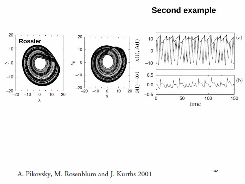
142

Rossler

Second example

143

x

HT[x]

x

y=HT[x]

Third example

Surface air temperature (SAT)

HT[sin(t)]=cos(t)

Zappala, Barreiro and Masoller, Entropy (2016)

http://www.mdpi.com/1099-4300/18/11/408/pdf

For a real time series x(t) defines an analytic signal

Hilbert transform

144

A word of warning:

Although formally a(t) and (t) can be defined for any x(t),

they have a clear physical meaning only if x(t) is a

narrow-band oscillatory signal: in that case, the a(t)

coincides with the envelope of x(t) and the instantaneous

frequency, (t)=d/dt, coincides with the dominant

frequency in the power spectrum.

145

Can we use the Hilbert amplitude, phase, frequency, to :

‒ Identify and quantify regional climate change?

‒ Investigate synchronization in climate data?

Problem: climate time series are not narrow-band.

Usual solution (e.g. brain signals): isolate a narrow

frequency band.

However, the Hilbert transform applied to Surface Air

Temperature time series yields meaningful insights.

Application to climate data

Hilbert phase dynamics: temporal evolution of the

cosine of the phase

Typical year El Niño year La Niña year

http://www.fisica.edu.uy/~cris/videos/map_typical.mp4

http://www.fisica.edu.uy/~cris/videos/map_ElNino.mp4

http://www.fisica.edu.uy/~cris/videos/map_LaNinal.mp4

The data:

Spatial resolution 2.50 x 2.50 10226 time series

Daily resolution 1979 – 2016 13700 data points

Where does the data come from?

European Centre for Medium-Range Weather Forecasts

(ECMWF, ERA-Interim).

Freely available.

“Features” extracted from each SAT time series

Time averaged amplitude, a

Time averaged frequency,

Standard deviations, a,

Changes in Hilbert amplitude and frequency detect

interdecadal variations in surface air temperature (SAT)

Relative decadal variations

Relative variation is considered significant if:

1979198820072016 aaa

19792016

a

a

ssa

a2.

ssa

a2.

or

100 “block” surrogates

D. A. Zappala, M. Barreiro and C. Masoller, “Quantifying changes in spatial

patterns of surface air temperature dynamics over several decades”,

Earth Syst. Dynam. 9, 383 (2018)

https://www.earth-syst-dynam-discuss.net/esd-2017-79/


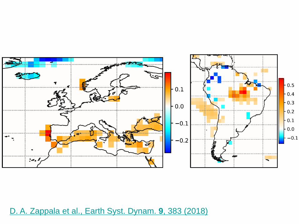
Relative variation of average Hilbert amplitude uncovers

regions where the seasonal cycle increased/decreased

Decrease of precipitation: the solar radiation that is not

used for evaporation is used to heat the ground.

Melting of sea ice: during winter the air temperature is

mitigated by the sea and tends to be more moderated.

o

D. A. Zappala et al., Earth Syst. Dynam. 9, 383 (2018)




Relative change of time-averaged Hilbert frequency

consistent with a north shift and enlargement of the

intertropical convergence zone (ITCZ)First ten years

Last ten years



Hilbert analysis combined

with temporal averaging:

another way to uncover

temporal regularity in data

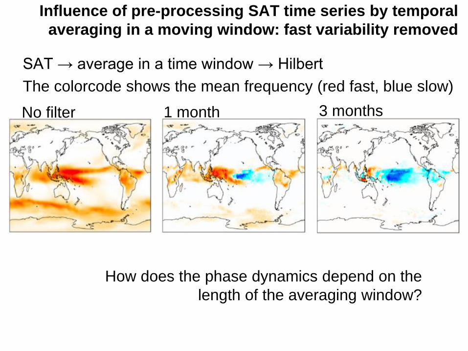
SAT → average in a time window → Hilbert

The colorcode shows the mean frequency (red fast, blue slow)

Influence of pre-processing SAT time series by temporal

averaging in a moving window: fast variability removed

No filter 1 month 3 months

How does the phase dynamics depend on the

length of the averaging window?

Mean rotation period (in years)

We will investigate some geographical locations: regular (circle),

quasi-regular (triangle), double period (square), irregular (plus),

El Niño (cross), quasi-biennial oscillation (QBO, star)

Variation of mean rotation period with the smoothing length

155

Regular, quasi-regular and double period sites: a plateau at 1 year is

found when increasing the averaging window (sooner or latter)

Irregular site: no plateau.

In El Niño and QBO sites: plateau at 4 and 2.5 years respectively.

Can we understand the variation of T with ?

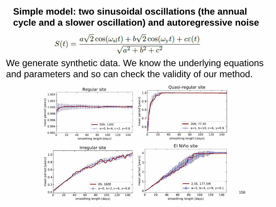
Simple model: two sinusoidal oscillations (the annual

cycle and a slower oscillation) and autoregressive noise

156

We generate synthetic data. We know the underlying equations

and parameters and so can check the validity of our method.

Phase-date relation:

Regular site

157

→Pre-filtering

SAT time

series in a

moving

window of

=41 days

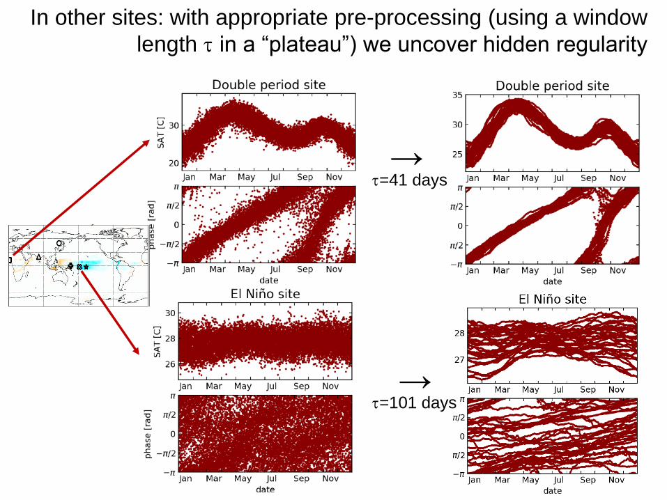
In other sites: with appropriate pre-processing (using a window

length in a “plateau”) we uncover hidden regularity

158

→=41 days

→=101 days

But in irregular site no plateau

159

→=101 days

Can we detect non-trivial underlying periodicities

with Fourier analysis?

No. The position of the main peak in the Fourier spectrum does not change,

or changes abruptly when increasing the length of the averaging window.

Classification of SAT dynamics using k-means clustering

161

Blue cluster: regions dominated by the seasonal cycle and large

temperature variations

Orange cluster: regions with fast dynamics that are dominated by the

annual cycle only after smoothing with > 20 days, which may reflect the

importance of subseasonal variability

Green cluster: regions of low temperature variability, whose spatial

structure is closely related to the mean rainfall pattern

Red cluster: relatively weak annual cycle and influenced by El Niño and

the QBO and thus shows slow dynamics

k-means clustering aims to partition n observations into k

clusters in which each observation belongs to the cluster with

the nearest mean.

k-means clustering

162

The goal is to minimize the

within-cluster sum of squares

Steps 2 and 3 are

repeated until

convergence has

been reached.

Source: Wikipedia

NP-hard problem, many free and licensed algorithms available.

And many more TS analysis

methods Wavelets

Detrended fluctuation analysis

Sample entropy, approximate entropy

Multifractality

Topological data analysis

Etc. etc.

There are MANY methods that return “features” that

characterize time series.

164

How to compare different methods?

How to identify similar time-series?

How to identify similar methods?

‒ HCTSA: highly comparative time-series analysis

‒ From each TS extracts over 7700 features

B. D. Fulcher, N. S. Jones: Automatic time-series phenotyping

using massive feature extraction. Cell Systems 5, 527 (2017).


165Matlab code: www.github.com/benfulcher/hctsa

What to do with more than

7700 features?

Let’s take a step back.

Assuming we have computed 120 ordinal probabilities.

What we do next?

167

O. A. Rosso et al, Phys. Rev. Lett. 99, 154102 (2007)

Many methods for reducing high-dimensional data to a

small number of dimensions.

Example:

Nonlinear dimensionality reduction (NLDR)

168

Each image of the letter 'A‘ has 32x32

pixels = vector of 1024 pixel valuesNLDR reduces the data into just two

dimensions (rotation and scale)

Source:

Wikipedia

A popular method: ISOMAP

A linear method: Principal Component Analysis (PCA)

Symbolic analysis, network representation, spatiotemporal

representation, etc., are useful tools for investigating

complex signals.

Different techniques provide complementary information.

Take home messages

“…nonlinear time-series analysis has been used to great

advantage on thousands of real and synthetic data sets from a

wide variety of systems ranging from roulette wheels to lasers to

the human heart. Even in cases where the data do not meet the

mathematical or algorithmic requirements, the results of

nonlinear time-series analysis can be helpful in understanding,

characterizing, and predicting dynamical systems…”

Bradley and Kantz, CHAOS 25, 097610 (2015)

References

170

Bandt and Pompe PRL 88, 174102 (2002)

U. Parlitz et al. Computers in Biology and Medicine 42, 319 (2012)

C. Masoller et al, NJP 17, 023068 (2015)

A. Aragoneses et al, PRL 116, 033902 (2016)


F. Arizmendi, Barreiro and Masoller, Sci. Rep. 7, 45676 (2017)

M. Panozzo et al, Chaos 27, 114315 (2017)

Zappala, Barreiro and Masoller, Entropy 18, 408 (2016)

Zappala, Barreiro and Masoller, Earth Syst. Dynam. 9, 383 (2018)

R. Hegger, H. Kantz and T. Schreiber, Nonlinear

Time Series Analysis (book and software TISEAN).


https://www.sciencedirect.com/science/article/pii/S0010482511000618




http://rdcu.be/qwUE


http://www.mdpi.com/1099-4300/18/11/408/pdf


https://www.pks.mpg.de/~tisean/

<[email protected]>

http://www.fisica.edu.uy/~cris/

Date post:	10-Jan-2020
Category:	Documents
Upload:	others
View:	8 times
Download:	0 times

Cristina Masoller - fisica.edu.uycris/teaching/slides_masoller_uni.pdf · Discrete Fourier...

Documents