Criteria for static equilibrium in particulate mechanics

computations

Xuxin Tu∗, Jose E. Andrade

Department of Civil and Environmental Engineering, Northwestern University,

Evanston, IL 60208, USA

Abstract

The underlying physics of granular matter can be clearly solved using particulate mechanics

methods, e.g., the discrete element method (DEM) that is inherently discontinuous and het-

erogeneous. To solve static problems, explicit schemes using dynamic relaxation procedures

have been widely employed, in which naturally dynamic material parameters are typically

adapted into pure numerical artifacts with the sole purpose of attaining meaningful results.

In discrete computations using these explicit schemes, algorithmic calibration is demanded

under general conditions in order to achieve quasi-static states. Until now, procedures for al-

gorithmic calibration have remained rather heuristic. This paper presents two criteria, using

the concept of homogenized stresses, for evaluating equilibrium in quasi-static applications of

particulate mechanics methods. It is shown, by way of numerical examples, that the criteria

for static equilibrium can be applied successfully to obtain quasi-static solutions in explicit

DEM codes through algorithmic calibrations. A general procedure is proposed herein for

carrying out the algorithmic calibration effectively and efficiently.

Keywords

static equilibrium, discrete element, homogenized stress, external stress, boundary stress,

algorithmic calibration∗Corresponding author. E-mail: x-tu@northwestern.edu

1 Introduction

Granular materials are ubiquitous in nature and in industry. In nature, granular materials

abound as they constitute the fundamental ingredients of many geomaterials, including soils,

rocks, and concrete. In industry, granular materials populate products in the pharmaceutical,

chemical, mining, agricultural, and food industries. Problems typically involve understanding

the mechanical behavior of such complex systems. In engineering, extraction of stress-strain

laws in these materials is of crucial importance for the understanding, modeling, and prediction

of engineering products. From a modeling standpoint, the finite element method constitutes

perhaps the most powerful and versatile tool for modeling engineering systems, including

granular media. However, it is clear that the behavior of granular systems is encoded at the

particle scale, propagating all the way to the macroscopic scale.

In an effort to develop the discrete mechanics for granular matter, Cundall and Strack [1]

proposed the discrete element method (DEM) in the late seventies. In DEM, rigid particles

are governed by Newtonian dynamics and are allowed to interact with each other by contact.

Due to its versatility, DEM has become an important tool in investigating micro-scale mecha-

nisms in granular materials [2; 3]. The method has captured the attention of many researchers

and has been used to model a plethora of materials such as rocks [4], asphalt mixtures [5],

concrete [6], and clays [7]. Industrial applications include modeling of chemical particles [8],

powders [9] and nanoparticles [10]. The method has also been used to investigate the effect

of shape (especially on the dilatancy properties of granular materials) including polyhedral

blocks [11], ellipsoids [12], and arbitrary shapes using overlapping rigid clusters [13]. Engi-

neering applications of the method include penetration of concrete targets [14], generation of

constitutive relations for granular materials [15; 16], investigation of the microscopic mech-

anism of shear banding [17], and simulation of fluidized beds, widely used in chemical and

industrial applications [8].

Perhaps, as pointed out by Ng [18], the beauty of DEM is its simplicity. However, in

many of the aforementioned applications (including in the pioneering work of Cundall and

Strack [1]) Newton’s equations are used to simulate steady-state or quasi-static conditions

2

where inertia terms typically vanish. Occasionally, input algorithmic parameters that be-

long to dynamic simulations (e.g., damping, fictitious mass) are assigned values without any

physical or mathematical justification, in some instances with the sole purpose of attaining a

steady-state solution. One could argue that computational expense and spurious parameter

calibration have prevented the method from penetrating practice further. In the case of com-

putational expense, it is expected that full-scale computations using DEM will be possible in

the next twenty years [19] and steps to accelerate that rate using multi-scale techniques and

hybrid approaches are already underway (see the works in [20] and [21]). The issue related to

parameter calibration is still unresolved and furnishes the motivation for this paper.

To solve static problems (omnipresent in engineering) using explicit schemes, ‘dynamic

relaxation’ procedures have been typically employed [22]. These procedures are based on

the fundamental idea, originally proposed by Rayleigh [23], that the static solution of a me-

chanical system can be viewed as the steady-state part of a corresponding dynamic problem.

This method was widely applied to finite difference and finite element methods especially in

non-linear structural analysis [24–26], and various algorithms were developed to automatically

adjust the algorithmic parameters [22; 27; 28]. Based on the conditions for optimal conver-

gence of dynamic relaxation [22] and the properties of the Rayleigh quotient, Bardet and

Proubet [29] proposed an adaptive algorithm for explicit discrete element methods, which has

demonstrated its success in randomly-packed assemblies. In contrast to a numerical method

used for continuum materials, however, the discrete element method encounters more vari-

ations and uncertainties in simulating an arbitrary granular system. Variations in particle

geometry, particle size distribution, contact law, contact forming and breaking, etc., are dif-

ficult to take into account in an adaptive algorithm for automatic parameter update. As a

result, algorithmic calibration, i.e., choosing values for the algorithmic parameters involved

in explicit DEM schemes, is generally required to perform quasi-static simulations. The crux

of the problem is the evaluation of static equilibrium in explicit DEM computations in the

context of quasi-static applications.

In this paper, criteria for the evaluation of static equilibrium are derived using a rather

3

general approach. It is shown that these criteria boil down to conservation of linear and

angular momenta in the ‘homogenized’ problem, following lines close to those proposed by

Christoffersen et al [30]. A general assembly of particles is forced to obey static equilibrium,

which will in turn imply conditions on the homogenized stress tensor. Even though the

conservation of momenta of the homogenized problem is not particularly new, the idea of

utilizing the implied qualities of the homogenized stress as necessary macroscopic criteria

for static equilibrium is novel. A further innovation in this paper is the use of the criteria

to systematically calibrate explicit DEM codes to achieve quasi-static states under general

conditions. In doing so, this paper contributes to the unresolved issue of parameter calibration

by proposing a framework bolstered by conditions of static equilibrium from the onset of

computation. We generalize our findings and outline a procedure for consistent algorithmic

calibration in DEM.

The organization of the paper is as follows. First, the most widely used explicit scheme for

DEM simulations and its algorithmic calibration is briefly described to illustrate the potential

issues arising in the numerical solution. Second, the necessary criteria for static equilibrium

in an arbitrary granular assembly are presented. Then, these criteria are used to calibrate a

‘benchmark’ example where parametric studies are performed to show the effects of deviating

from the ‘optimal’ parameters. Finally, a general procedure for calibration of explicit DEM

codes for quasi-static applications is presented and some conclusions based on our findings

are drawn.

As for notations and symbols used in this paper, bold-faced letters denote tensors and

vectors; the symbol ‘·’ denotes an inner product of two vectors (e.g. a · b = aibi), or a single

contraction of adjacent indices of two tensors (e.g. c · d = cijdjk); the symbol ‘⊗’ denotes a

juxtaposition, e.g., (a⊗ b)ij = aibj and the symbol ‘×’ denotes a cross product between two

vectors, e.g., (a× b)k = εijkaibj , where εijk is the permutation operator.

4

2 DEM schemes and algorithmic calibration

As mentioned in the introduction, DEM codes are often used to model quasi-static engineering

problems. However, to achieve quasi-static states in explicit DEM schemes, the algorithmic

parameters involved must be properly calibrated, a procedure typically referred to as algorith-

mic calibration. Without algorithmic calibration, the explicit method tends to yield erroneous

results and thus becomes useless. Unfortunately, algorithmic calibration is generally ignored

in practice and the involved parameters are often assigned on an arbitrary basis, which has

made it difficult to compare results from different sources and could undermine the scientific

value of the reported data. Therefore, it is crucial to regularize the algorithmic calibration

for the explicit DEM scheme.

To this end, there are two fundamental questions to be answered. First, what criteria

should be used to effectively evaluate convergence of the numerical scheme to quasi-static

equilibrium? In particulate mechanics methods, it is always possible to evaluate equilibrium

for each individual particle. However, it is not desirable to evaluate the balance of a system

directly based on individual evaluations. Sometimes, the overall kinetic energy is employed

to judge if a granular system reaches quasi-static states. Nevertheless, zero kinetic energy

does not necessarily infer quasi-static equilibrium. The second fundamental question is: what

procedure should one follow to perform the algorithmic calibration? These two questions are

interconnected; one can use the criteria both to consistently enforce static equilibrium and to

systematically calibrate explicit DEM schemes for static applications.

In order to begin answering the aforementioned questions, it is first necessary to under-

stand the underlying methodology used in explicit DEM codes and their intimate dependence

on the algorithmic parameters used. The subsequent sections outline some of these issues.

2.1 Particle interactions and governing equations

In DEM, interparticle interactions are typically treated in normal and tangential components

at contact points. In the normal direction, the normal force fn is related to the normal

5

displacement δn such that

fn = knδn (2.1)

where kn is the normal contact stiffness. To obtain more realistic results, Herzian normal

contact law [31] is usually employed, with kn expressed as

kn =Eµ

√2rδn

3(1− ν2µ)

(2.2)

where r is the radius of particle, Eµ is the Young’s modulus and νµ is the Poisson’s ratio

of the particles. In this work, only elastic normal contact is considered. In the tangential

direction, the tangential force ft is related to the tangential displacement δt. Using the

Coulomb frictional law, a general expression for a tangential contact model reads

ft = min(kt|δt|, tanφµfn)δt

|δt|(2.3)

where kt is the tangential contact stiffness and φµ is the intergranular friction angle. According

to Mindlin and Deresiewicz [32], kt is related to kn via

kt =3(1− νµ)2− νµ

kn (2.4)

In light of the force-displacement laws outlined above, each contact can be idealized as

two springs in the normal and tangential directions, as shown in Figure 1. By perturbing

an individual particle while fixing its neighboring particles, the governing equation for this

particle—in static equilibrium—can be expressed as

Kp · up = fp (2.5)

where Kp, the local stiffness matrix, assembles the stiffness contribution from each contact

on the particle, while up and fp are the generalized displacement vector and force vector,

respectively. The dimension of up, or fp, corresponds to the number of degrees of freedom

6

(DOF), denoted by Ndof . For a 2D problem, Ndof = 3, corresponding to two translation

DOFs and one rotation DOF. Hence the term ‘generalized’ is used for naming up and fp. For

a translation DOF, the corresponding component of fp is a measure of force. On the other

hand, for a rotation DOF, it is a measure of moment. For a nonlinear relation, such as the

Herzian contact law, Kp is a function of kn, kt and φµ at each contact point. Therefore, Kp is

dependent on the particle displacement u and equation (2.5) represents a generally nonlinear

relation. An example of how to construct the local stiffness matrix can be found in the work

of van Baars [33].

Figure 1: Equivalent mass-spring system for an individual particle within a granular system.

Assembling equation (2.5) over all particles in the granular system yields

K · u = f ext (2.6)

where K is the global stiffness matrix with dimensions (Np ×Ndof) × (Np ×Ndof) with Np

as the total number of particles in the system, u is the global displacement vector, and f ext

is the external force vector—the counterpart of the internal force vector f int, which is equal

to the left hand side of equation (2.6). The global entities in equation (2.6) are assembled

from their local counterparts Kp, up and fp in a procedure similar to that followed in FEM

to obtain global arrays based on local arrays [34; 35]. Effectively, equation (2.6) defines the

governing equation for any granular system under static equilibrium, which often is simply

expressed as

f tot = f ext − f int = 0 (2.7)

7

N

Y

ext rmationsloads/defo prescribed nf⇒

t

t

kk

kk

kkk

∆=∆

∆=

⋅−⋅

++

++

+

11

11

tot-11 )(＝

uu

uu

uDfMu

&

&&&

&&&

? tot TOLk <f

int1

ext1

tot1

11int

1

11

+++

+++

++

−=

⋅=

∆+=

kkk

kkk

kkk

fff

uKf

uuuStage 1 Stage 2

intexttotnnk

0k fff −=

=

1kk +=

intint

1

kn

nn

(a) (b)

f=

+=

f

N

Y

ext rmationsloads/defo prescribed nf⇒

t

t

kk

kk

kkk

∆=∆

∆=

⋅−⋅

++

++

+

11

11

tot-11 )(＝

uu

uu

uDfMu

&

&&&

&&&

? tot TOLk <f

int1

ext1

tot1

11int

1

11

+++

+++

++

−=

⋅=

∆+=

kkk

kkk

kkk

fff

uKf

uuuStage 1 Stage 2

intexttotnnk

0k fff −=

=

1kk +=

intint

1

kn

nnf=

+= f

ext rmationsloads/defo prescribed nf⇒

t

t

nn

nn

nnn

∆=∆

∆=

⋅−⋅

++

++

+

11

11

tot-11 )(＝

uu

uu

uDfMu

&

&&&

&&&

11int

1

11

+++

++

⋅=

∆+=

nnn

nnn

uKf

uuu

Stage 1Stage 2

intexttot nnn fff −= 1nn +=

ext rmationsloads/defo prescribed nf⇒

t

t

nn

nn

nnn

∆=∆

∆=

⋅−⋅

++

++

+

11

11

tot-11 )(＝

uu

uu

uDfMu

&

&&&

&&&

11int

1

11

+++

++

⋅=

∆+=

nnn

nnn

uKf

uuu

Stage 1Stage 2

intexttot nnn fff −= 1nn +=

Figure 2: Flowcharts of two typical explicit schemes for static DEM: (a) iterative scheme, and(b) stationary scheme.

2.2 Motion equations and explicit schemes

Equations (2.6) and (2.7) bear a great resemblance to the matrix form of static FEM and

can be solved using an implicit scheme [33]. In practice, however, explicit schemes using

dynmaic relaxation procedures [22] are greatly preferred for solving DEM systems, due to

their simplicity and claimed computational inexpensiveness [36].

Figure 2 shows two prototypical explicit schemes used for static DEM, with the first being

iterative and the second being stationary. In either scheme, the overall progress is controlled

by prescribed loads or displacements, which are added incrementally. The subscript n denotes

the step number (used in both schemes) while the subscript k indicates the iteration number

(used only in the iterative scheme). From Figure 2, it can be seen that the cores of these

two schemes, outlined by the dashed lines, consist of two stages and are quite similar to each

other. For the iterative scheme, the first stage employs the following set of motion equations

with damping to compute ∆u, the correction to the particle displacement, given f totk , the

unbalanced force resulting from the last iteration,

uk+1 = M−1 ·(f tot

k −D · uk

); uk+1 = uk+1∆t; ∆uk+1 = uk+1∆t (2.8)

where u and u are the generalized acceleration and velocity, respectively; M is the mass

8

matrix containing the fictitious mass [29] for each particle; D is the damping matrix composed

of damping coefficients for each particle in each DOF and ∆t is the time step. In the second

stage, shown in Figure 2a, the displacement vector u is updated. Then, the contact stiffness K

and the internal force vector f int are updated based on the new value of u. Subsequently, the

total force vector f tot is reevaluated. This two-stage procedure is repeated until the total or

unbalanced force f tot is dissipated, i.e., ‖f tot‖ is less than a small number, typically assigned

in an arbitrary manner. Note that the stiffness matrix K is not actually assembled in explicit

DEM schemes. It is used here for a concise mathematical presentation since updating every

individual contact stiffness is equivalent to updating the overall stiffness.

The stationary scheme differs from the iterative scheme in two main aspects. First, the

two-stage procedure in the former scheme is invoked only once for each increment of prescribed

boundary conditions. Second, the magnitude of the increment in the stationary scheme is

generally much smaller than that in the iterative scheme. Despite the differences, both schemes

aim to achieve quasi-static states. Their relation is analogous to that between a stepwise

consolidation test and a gradual consolidation test in soil mechanics. In the former test,

vertical loads are added in finite steps and a relatively long period of time is placed between

consecutive steps to allow excess pore pressure to dissipate. In the latter case, loads are

gradually increased at a slow rate, which can be regarded as using a large number of small

steps to exert the same amount of total load within the same period of time. In the numerical

schemes, the counterpart of the excess pore pressure is the kinetic energy introduced by the

procedure of dynamic relaxation.

In fact, the stationary explicit scheme for static DEM is form-identical to an explicit

scheme for dynamic DEM, which solves the following governing equation,

M · u + D · u + K · u = f ext (2.9)

To solve this dynamic problem, the scheme depicted in Figure 2b can be used. Nevertheless,

these two schemes are fundamentally different. The scheme for dynamic DEM faithfully de-

scribes the physics of particles under dynamic conditions. Therefore, the parameters involved

9

therein must truly represent the real material properties. For instance, the damping D should

be ideally measured from relevant experiments. In contrast, most parameters involved in the

static DEM scheme, including M , D, ∆t, etc., serve as pure numerical artifacts and generally

have no relation to their physical counterparts. For instance, the fictitious mass is often up-

scaled by orders of magnitude in static DEM to reduce dynamic effects [37]. Their values are

assigned with the sole purpose of achieving quasi-static states, i.e., dissipating kinetic energy

while balancing external forces throughout the particulate system.

2.3 Algorithmic calibration

From the previous discussions, it becomes clear that equation (2.6) is the governing equation

to be solved in any static problem, while equation (2.9) represents the dynamic relaxation

procedure employed by explicit schemes to converge to the governing equation. However,

the dynamic relaxation does not necessarily guarantee that equation (2.6) can be recovered.

In fact, it is easy to obtain erroneous results using explicit DEM schemes, if the involved

algorithmic parameters are simply assigned on an arbitrary basis.

According to equation (2.8), the displacement correction algorithm used in explicit schemes

essentially is given by the following relation,

∆uk+1 = M−1 ·(f tot

k −D · uk

)(∆t)2 (2.10)

Hence, this algorithm is affected by the chosen algorithmic parameters: the fictitious mass

M , the damping D and the time step ∆t. Their effects on the quality of solution are best

illustrated in a 1-DOF system under 1-D conditions. As shown in Figure 3, m, D, u and f

represent the scalar counterparts of M , D, u and f , respectively. The bold curves indicate

the relation between the static total force and the particle displacement, which is governed by

contact stiffness. The quasi-static solution u∗ corresponds to certain external force prescribed

on the system. As shown in Figure 3a, if the value of D is not assigned appropriately, Du

might exceed f tot. As a result, ∆u will diverge from the quasi-static solution u∗ during the

dynamic relaxation. Even if the displacement is updated in the right direction, as shown in

10

Figure 3b, wherein (f tot−Du) is positive, improper assignment of the algorithmic parameters

could lead to an extremely slow update rate, effectively rendering the method useless. For

example, if (f tot−Du) is relatively small or (∆t)2/m is relatively large, a slow convergence rate

can be expected. In a stationary explicit scheme, note that u∗ will evolve as the external load

increases. With inappropriate parameters, the displacement update might keep lagging behind

load increments, and quasi-static states might never be achieved. In fact, the loading rate,

indicating how ‘fast’ the boundary conditions are applied, is another algorithmic parameter

that affects the quality of the explicit scheme for solving static problems, and it will be

discussed later.

uk+1

f tot

u0 uk

fktot

u*1

uk1

D uk

t 2

m

(b)

fktot

(a)f tot

u0

u*uk1

D uk

1

t 2

m

uk+1

uk

Figure 3: Two scenarios for displacement update using dynamic relaxation: (a) update awayfrom static equilibrium; (b) update toward static equilibrium.

Therefore, it is clear that if the algorithmic parameters used in explicit DEM, such as

damping, fictitious mass, time step and loading rate, are not calibrated appropriately for the

quasi-static range, the numerical solutions obtained will be erroneous. Unfortunately, there

was no general procedure available to quantify static equilibrium and to calibrate algorith-

mic parameters for the quasi-static regime. The following sections outline a very promising

framework to answer the two questions posed at the beginning, i.e., what criteria should be

used to evaluate the quasi-static state in the explicit scheme, and how should the calibration

be performed using these criteria. It turns out that appropriate criteria to enforce static

equilibrium in an assembly of grains can be systematically utilized to calibrate algorithmic

parameters in explicit DEM codes.

11

Figure 4: Internal and external forces on particles.

Remark 1. The algorithmic calibration discussed in this paper should be distinguished from

the material calibration procedure commonly used in DEM simulations, in which the ma-

terial parameters (e.g., Eµ, νµ, φµ, etc.) are adjusted so that computed responses match

experimental observations.

3 Criteria for static equilibrium

For an individual particle within a granular assembly subjected to external tractions and body

forces, the balance of linear and angular momenta necessitates,

∑ncα=1 fα + t + b = 0∑nc

α=1 lα × fα + h× t = 0(3.1)

where nc is the total number of contacts acting on the particle, and the superscript α denotes

the αth contact. As illustrated in Figure 4, fα is the contact force at contact α, which is

an internal force, t is the external force acting on the boundary, b is the body force, lα is

the distance vector emanating from the centroid of the particle to the contact point α, and

h is the distance vector emanating from the centroid of the particle to the point where t is

exerted.

12

Summing equation (3.1) over all particles yields,

∑Ntβ=1 tβ +

∑Np

p=1 bp = 0∑Ntβ=1 hβ × tβ +

∑Np

p=1

∑ncα=1 lpα × fpα = 0

(3.2)

where Np is the total number of particles, and Nt is the total number of external forces

imposed on the boundary. Note that both l and h are reckoned with respect to the centroids

of the corresponding particles. Equation (3.2) designates the conditions for static force and

static moment balances. However, equation (3.2) does not serve as a desirable criterion,

because the force measures therein depend on the size of the assembly and thus they do not

represent average mechanical states of the assembly.

3.1 Homogenized stress and external stress

To describe the stress state of a particulate assembly, an average stress tensor, herein re-

ferred to as the homogenized stress, has been derived and has been frequently used in the

micromechanics of granular materials [30; 38–40]. However, its properties related to static

equilibrium have not been clearly pointed out and thus have not been fully utilized. It will be

shown that the most important qualities of the homogenized stress can be used as criteria to

evaluate static equilibrium. These properties are inferred from the mathematical derivation

of the homogenized stress, starting from the application of the principle of virtual work to

the internal and external forces in static balance:

Nc∑α=1

fα ·∆α +Nt∑

β=1

tβ · uβ +Np∑p=1

bp · up = 0 (3.3)

where ∆α is the virtual displacement at contact α; uβ is the virtual displacement at the point

β where the traction tβ is applied; up is the virtual displacement at the particle centroid and

Nc, Nt and Np are the total numbers of contacts, boundary forces and particles, respectively.

As shown in Figure 4, the particulate system can be enveloped by a smooth surface S,

on which it is always possible to replace the boundary force t with some equivalent traction

13

T , as typically done in continuum mechanics. Similarly, the body force b can be replaced

by some equivalent force density B for a continuum entity mechanically equivalent to the

particulate system. Therefore,

Nc∑α=1

fα ·∆α +∫

ST · u dS +

∫V

B · u dV = 0 (3.4)

where V is enclosed by S. Suppose the virtual displacement field u is a linear function of the

particle position x,

u = φ · x + c (3.5)

where the tensor φ and the vector c are arbitrary and constant, while the particle coordinates

x are evaluated at the centroid of the particle. For two particles A and B in contact at point

α, the virtual displacement ∆α can be computed as follows,

∆α = uA − uB = −φ · dα (3.6)

where uA and uB are virtual displacements of the two particles, the contact force fα equals

the force applied on particle A, and dα is the vector emanating from the centroid of A to the

centroid of B, as illustrated in Figure 4. Substituting equations (3.5) and (3.6) into (3.4),

and invoking the divergence theorem and the condition of static equilibrium, it can be shown

that

−Nc∑

α=1

fα ⊗ dα +∫

Vσ dV = 0 (3.7)

where σ is the local stress tensor for the equivalent continuum domain. Consequently, the

homogenized stress tensor is obtained, i.e.,

σ =1V

Nc∑α=1

fα ⊗ dα (3.8)

This homogenized stress has two important properties related to linear and angular momenta,

described in Sections 3.2 and 3.3 below.

14

3.2 Balance of linear momentum

By substituting equations. (3.5) and (3.6) into (3.3), it can be shown that

1V

Nc∑α=1

fα ⊗ dα =1V

Nt∑β=1

tβ ⊗ xβ +Np∑p=1

bp ⊗ xp

(3.9)

Both xβ and xp are position vectors locating the centroid of a particle, while xβ specifically

refers to the particle on which tβ is applied. The right hand side of equation (3.9) is defined

here as the external stress,

e =1V

Nt∑β=1

tβ ⊗ xβ +Np∑p=1

bp ⊗ xp

(3.10)

Using the definition given in equation (3.8), one concludes that

σ = e (3.11)

In essence, the homogenized stress represents an average of internal forces, while the external

stress represents an average of external forces. When the body force is ignored, as is frequently

done in practice, the resulting expression for the external stress becomes

b =1V

Nt∑β=1

tβ ⊗ xβ (3.12)

where b is referred to as the boundary stress. Then equation (3.11) reduces to

σ = b (3.13)

Equation (3.11), or (3.13), constitutes a reduced expression for the balance of linear mo-

mentum in a general granular assembly and serves as an alternative and partial expression

for equation (2.7). The former equation only involves translation DOFs according to its

derivation, while the force vectors in the latter equation are generalized, i.e., they include

15

components for both translation and rotation DOFs. The advantage of the expression in

equation (3.11) is that it is independent of the size of the granular assembly. Based on the

derivation shown above, equation (3.11) is a necessary condition for static equilibrium. As dis-

cussed later in Section 4.1, equation (3.11) can serve as an unambiguous criterion, if evaluated

on a systematic basis in quasi-static simulations involving DEM.

3.3 Balance of angular momentum

Rearranging the second term of the moment balance condition in equation (3.2), and express-

ing it in terms of the number of contacts instead of the number of particles, it can be shown

thatNt∑

β=1

hβ × tβ +Nc∑

α=1

dα × fα = 0 (3.14)

As pointed out by Bardet and Vardoulakis [41], the first term of equation (3.14) is generally

nonzero, but its relative significance decreases as the size of the particle system increases. For

a large particulate assembly, it is generally negligible. In addition, when uniform regularly

packed particles are tested under uniform and symmetric loads,∑Nt

β=1 hβ × tβ = 0, even for

a small number of particles. Under these circumstances,

Nc∑α=1

dα × fα = 0 (3.15)

Using the properties of the cross product plus equation (3.8), the homogenized stress is found

to be symmetric due to balance of angular momentum, i.e.,

σ = σT (3.16)

This equation is an alternative expression of equation (2.7) with respect to the rotation DOFs.

As a necessary condition, equation (3.16) itself does not rigorously infer balance of angular

momentum. Similar to equation (3.11), however, a systematic monitoring of equation (3.16)

in explicit DEM schemes can make it an effective criterion to evaluate the static balance of mo-

16

ments. Equation (3.11) and equation (3.16) furnish a complete set of criteria to evaluate static

equilibrium in quasi-static DEM simulations. These criteria will be used in the subsequent

sections to provide a systematic framework for i) assessing quasi-static conditions in DEM

simulations and ii) unambiguously performing algorithmic calibration, achieving algorithmic

parameters yielding meaningful numerical results.

Remark 2. The conventional homogenized stress σ is not the only expression to represent the

average stress state of a particulate assembly. For instance, Chang and Kuhn [42] derived an

average stress that is quite similar to σ but is generally symmetric. Using equation (3.9), if

both sides of equation (3.9) add an identical term so that xβ refers to the point where the

external force fβ is applied, instead of the particle centroid, then the resulting quantity on the

left hand side of equation (3.9) becomes an ideally symmetric stress measure. The interested

reader is referred to [42] for a more rigorous derivation and detailed discussion. Note that the

idea of using homogenized-stress-based criteria to evaluate quasi-static states in particulate

mechanics methods is not limited to the conventional homogenized stress σ. Using the average

stress derived by Chang and Kuhn, a set of criteria similar to equations (3.11) and (3.16) can

be derived as well, in which the external stress will be modified accordingly.

4 Numerical examples and parametric studies

Now that the criteria for static equilibrium have been determined, the issue of how to perform

algorithmic calibration using these criteria can be addressed. Before presenting an optimal

procedure for the calibration process, it is worth performing a parametric study to investigate

the effect of each major algorithmic parameter on the quality of the numerical solution. Several

important purposes are served by such a study. First, it helps explain how to use the proposed

criteria to evaluate quasi-static states in a systematic manner. Furthermore, development of a

general procedure for the algorithmic calibration relies heavily on understanding the effect of

each individual parameter. Finally, the parametric study demonstrates possible consequences

resulting from performing algorithmic calibration improperly, which reiterates the significance

of the criteria developed herein and the importance of regularizing algorithmic calibrations

17

for explicit DEM schemes.

4.1 Systematic evaluation of the criteria

As pointed out in Section 3, the two proposed criteria are necessary conditions of static

equlibrium. Satisfaction of these criteria at a given time instant does not necessarily infer

static equilibrium. For example, a particulate assembly in an oscillating state might satisfy

both criteria at a certain time instant. However, if these two criteria are evaluated constantly

throughout a loading period (e.g., using a series of monitoring points prescribed at small and

uniform time intervals, described herein as ‘systematically’), and if satisfaction of these two

criteria is constantly confirmed at each monitoring point, then it becomes a ‘high-probability-

event’ that quasi-static equilibrium has been achieved. The systematic monitoring can be

easily implemented in DEM codes by recording the homogenized stress σij and the external

stress eij periodically. Examples will be shown in the subsequent subsections on how to

systematically assess the quasi-static conditions using the proposed criteria.

4.2 Numerical specimen and experiment

The DEM code used in this study adopts the stationary explicit scheme introduced in Sec-

tion 2.2. Note that algorithmic calibrations need to be performed for both the iterative and

the stationary schemes to achieve quasi-static conditions, and both need rigorous criteria to

guide the calibrations. The findings of the parametric study presented herein are applicable

to iterative schemes as well.

Using the stationary explicit scheme, a series of numerical experiments with various algo-

rithmic parameters have been conducted on regularly-packed particulate assemblies to produce

stress-strain responses under plane strain conditions. In all cases, the numerical specimen is

composed of a single layer of uniform spherical particles in plane. Figure 5a shows the struc-

ture of the regular packing, which is characterized by the parameter α, herein referred to as

the packing angle. The numbers of the particles located on the two perpendicular bound-

aries, N1 and N3, designate the size of the assembly. Figure 5b shows the imposed boundary

18

Figure 5: Setup of numerical experiments.

conditions for the experiment, in which the top of the specimen is pushed by a rigid ‘platen’,

moving downwards at a prescribed rate. The lateral confinement is kept constant by imposing

constant forces evenly distributed on the particles located on the lateral boundaries.

In this parametric study, the uniform particle diameter is 1.5 mm. The size of the assembly

is 10 × 10, i.e., N1 = N3 = 10. The structural angle α = 30◦, corresponds to dense packing.

Each particle has the same material properties, with a Young’s modulus Eµ = 69 GPa, a

Poisson’s ratio νµ = 0.3 and an intergranular friction angle φµ = 30◦. The material density

is 2700 kg/m3, and gravity is ignored. As a result, the external stress equals the boundary

stress, i.e., b = e, cf. equations (3.10) and (3.12). There is no friction on the boundary of

the specimen. The total prescribed vertical displacement of the upper ‘platen’ is 0.05 mm,

corresponding to a total vertical strain of 0.18%. Throughout an ‘experiment’, the equivalent

lateral stress σ3 = 50 kPa.

One advantage of using regular packing is that an analytical solution exists for the strength

of the particulate assembly. Utilizing the condition for sliding at contact points and the

symmetry of the packing structure, it can be shown that the maximum stress ratio that can

be sustained by the assembly is given by

σ1

σ3

∣∣∣∣max

= cot(α− φµ)2 cos α + 1/N3

2 sinα + 1/N1(4.1)

19

As N1 and N3 grow, equation (4.1) will approach the analytical solution given by Rowe [43]

σ1

σ3

∣∣∣∣max

= cot(α− φµ) cot α (4.2)

For the problem concerned in this parametric study, σ1max = 352 kPa. This value serves as

an extra and important measure, in addition to the proposed criteria, to evaluate the results

obtained from the ‘experiments’, which will be discussed subsequently.

4.3 Initial values for calibration

The algorithmic parameters involved in the explicit scheme applied herein include the loading

rate, the time step, the fictitious mass and the damping. For simplicity, all particles in the

assembly have the same fictitious mass m and the same damping coefficients Dt and Dr

corresponding to the translational and rotational DOFs, respectively. As a typical trial-and-

error process, the algorithmic calibration of the explicit DEM scheme starts with certain initial

values for the algorithmic parameters. Unless a mass scaling method [37] is used, the fictitous

mass m typically equals the actual particle mass mp. For choosing proper initial values for

other parameters, there exist a number of guidelines based on previous research.

The upper bound of the time step is limited by the critical time step ∆tcrit. For a linear

undamped system solved using an explicit scheme, ∆tcrit is given by

∆tcrit =2√

λmax(4.3)

where λmax denotes the maximum eigenvalue of the M−1K matrix [34; 44], while the mass

matrix M and the stiffness matrix K have been defined in the previous section. Note that

equation (4.3) only applies to undamped systems and K is not actually assembled in explicit

DEM schemes. Therefore, it is not desirable to use equation (4.3) to estimate the initial value

for the time step. For a 1-D generalized mass-spring system, the critical time step is simply

given by

∆tcrit = 2√

mg/kg (4.4)

20

where mg and kg represent the generalized mass and the generalized spring stiffness, respec-

tively. Equation (4.4) is a common starting point for numerous ad hoc methods for determin-

ing an ‘effective mass’ and ‘effective stiffness’. Dependent upon the complexity of the analyzed

system and the treatment of damping, such approaches usually necessitate an additional time

step reduction parameter so that stable computations can be carried out [18; 36]. As will

be shown subsequently, this reduction parameter can be obtained by applying the criteria

proposed herein.

To approach the critical time step for a DEM system, mg and kg in equation (4.4) should

correspond to their minimum and maximum values, respectively. Note that mg and kg are

generalized measures. For a translation DOF system, mg refers to the particle mass mp, while

kg is equal to kn defined in equation (2.1). For a rotation DOF system, i.e., a mass allowed

to rotate around its centroid, mg represents the moment of inertia of the particle, equal to

2mpr2/5 for spheres with r denoting the particle radius, while kg = ktr

2 with kt defined in

equation (2.3). Let ∆tcritt denote the critical time step computed for translation DOFs and

∆tcritr denote that computed for rotation DOFs. For spherical particles, it can be shown that

∆tcritr < ∆tcritt . Therefore,

∆tcrit = ∆tcritr = 2√

(2mp)/(5kt) (4.5)

For a nonlinear contact model, like those introduced in Section 2.1, kt depends on the contact

displacement δn. In this study, the maximum stiffness is used to calculate ∆tcrit by using the

maximum value of δn encountered in a computation.

For a 1-D generalized mass-spring-damper system, a critical damping coefficient exists,

which enables the system to return to its balanced state faster than any other damping

coefficient and without oscillation. For a translation DOF system, the critical damping is

given by

Dcritt = 2

√mpkn (4.6)

21

and for a rotation DOF system,

Dcritr = 2r2

√2mpkt/5 (4.7)

Note that Dcritt and Dcrit

r have different units and apply to the two different DOFs, respectively.

In this study, since the total vertical displacement has been prescribed, the loading rate

is represented by the total step number Nstep. The larger Nstep is, the lower the loading

rate will be. Although there is no rigorously derived critical value available for Nstep, the

parametric study presented herein will provide useful information for choosing an appropriate

initial value for Nstep.

4.4 Benchmark case

Figure 6 plots the homogenized stress and the boundary stress versus vertical strain obtained

from a successfully completed calibration. The purpose here is to set up a benchmark case, to

which the results from other computations using non-optimal algorithmic parameters can be

compared. The calibration procedure will be discussed in the next section. For the vertical

components, the σyy curve closely matches the byy curve, indicating a well-maintained force

balance in that direction. Meanwhile, the computed peak vertical stress is close to 352 kPa,

the analytical solution, marked by a black arrow in the figure. For the horizontal components,

σxx is constantly equal to 50 kPa, the prescribed lateral stress, indicating a horizontal force

balance. For the shear stress components, both σxy and σyx are relatively small (< 1.5 kPa).

For an even smaller particle assembly, it has been shown that the shear stress components can

be as small as 5× 10−10 kPa under a similar loading condition [45], which generally does not

happen in larger systems. In Figure 6, σxy and σyx very closely match one another throughout

the simulation, indicating a persistent balance of moments. Hence, the two criteria for static

equilibrium are systematically satisfied, which is additionally verified by the match between

the computed and the analytical solutions for the peak strength. In conclusion, the quasi-

static states have been successfully achieved throughout the computation in this benchmark

case.

22

Figure 6: Normal (a) and shear (b) stresses plotted versus vertical strain for the ‘benchmark’computation.

The optimized values for the four algorithmic parameters are ∆tbm = 0.2∆tcrit, Dbmt =

Dcritt , Dbm

r = Dcritr and Nbm

step = 3 × 105, where the superscript ‘bm’ indicates ‘benchmark’.

Mass scaling has not been used, and therefore the fictitious mass equals the actual particle

mass. Note that the data shown in Figure 6 corresponds to 100 monitoring instants evenly

spaced throughout the ‘experiment’. Compared to the applied Nstep value, the computation

cost due to the systematic monitoring is negligible.

4.5 Loading rate

As mentioned before, the loading rate refers to the magnitude of load or displacement pre-

scribed per unit time step. The loading rate and the time step are two independent algorithmic

parameters in explicit schemes. Unlike other algorithmic parameters, the loading rate has not

gained much attention in DEM applications. A large loading rate tends to make the computed

response dynamic rather than quasi-static. As an extreme case, a large strain, say, of 1%,

would result in an unreasonably large contact force if applied to a particulate assembly in just

one step. Using the contact model introduced in Section 2.1, extremely large particle velocity

will be generated via the motion equations, making the entire computation meaningless. Note

that this effect of the loading rate on the computed results applies to both the iterative and

the stationary explicit schemes for DEM (cf. Section 2).

23

Figure 7: Effect of loading rate (Nstep varied for a total vertical strain equal to 0.18%). (a)and (b): Nstep = Nbm

step/6 = 5× 104; (c) and (d): Nstep = (100/3)Nbmstep = 107

Figures 7a and 7b show a computation using an Nstep that is one sixth of the Nbmstep, with

the other parameters equal to their benchmark values. Though σxy mostly matches σyx in

Figure 7b, it can be seen from Figure 7a that there is significant gap between byy and σyy,

indicating an unbalanced force in the vertical direction. Compared to the analytical solution,

the peak strength is overpredicted. Furthermore, the post-peak stress-strain response clearly

differs from that observed in the benchmark case. This case verifies that the loading rate has

an upper bound (or Nstep has a lower bound) for the quasi-static regime.

It might not be as straightforward to realize that there exists a lower bound for the loading

rate. Figures 7c and 7d show a computation using an Nstep about 33 times that of Nbmstep.

In this case, σxy and σyx are closer to zero, which is good. However, the computed strength

24

of the material is significantly lower than the analytical solution. An interesting observation

in Figure 7c is that a zigzag pattern is legible in both the byy and σyy curves which mostly

coincide with each other. This pattern is different from the noise introduced by transient

effects, where byy and σyy typically do not match, as will be shown in subsequent cases.

In summary, both upper and lower bounds exist for the loading rate. Thus, Cundall and

Strack’s suggestion that “the departure from equilibrium may be made as small as desired by

reducing the applied loading rate”[1] should be heeded with careful understanding.

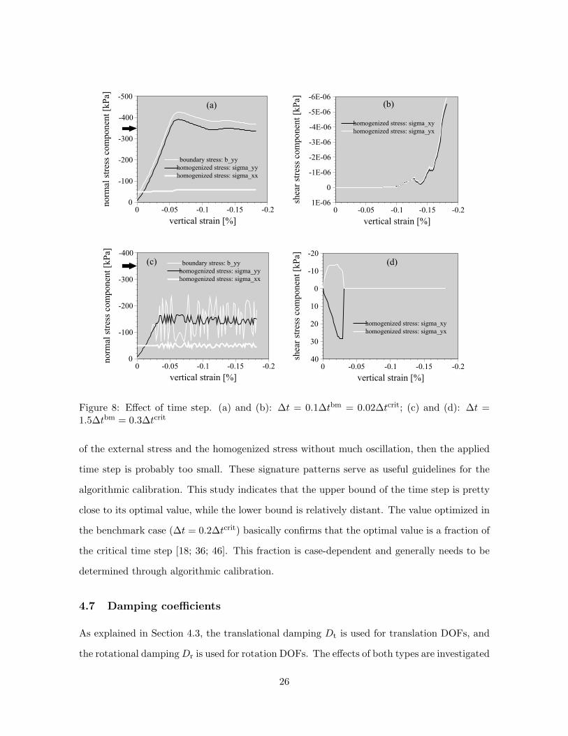
4.6 Time step

As discussed in Section 4.3, the time step should not be too large. But this does not necessarily

mean that smaller time steps are always better. Figures 8a and 8b show a computation using

a ∆t that is one tenth of ∆tbm with the other parameters equal to their benchmark values.

Similar to what was observed in the previous case, a significant gap exists between byy and σyy.

In addition, the strength of the numerical specimen is overpredicted, indicating an unbalanced

system and a spurious result. Therefore, there exists a lower bound of ∆t for obtaining

quasi-static conditions, which should not be confused with the situation of a dynamic DEM

application. In the latter case, ∆t is only limited by the stability consideration, while smaller

time steps always make computed results closer to the exact solution. The bottom line is that

the dynamic effect will not be reduced by reducing the time step.

Certainly, the upper bound cannot exceed the critical time step, but how close is it to

the critical value? Figures 8c and 8d plot the data from a computation using a ∆t that is

1.5 times that of ∆tbm, which is 30% of ∆tcrit. As shown, the peak vertical stress computed

is significantly lower than 352 kPa, the analytical solution, and the post-peak behavior is

overwhelmed by oscillation. Furthermore, the shear stresses are relatively large and σxy is

oppositely different from σyx. All of these observations are indicative of unbalanced forces

and moments.

With the other parameters in the neighbourhood of their optimal values, detection of

excessive oscillation indicates that the applied time step is too large. If there is a separation

25

Figure 8: Effect of time step. (a) and (b): ∆t = 0.1∆tbm = 0.02∆tcrit; (c) and (d): ∆t =1.5∆tbm = 0.3∆tcrit

of the external stress and the homogenized stress without much oscillation, then the applied

time step is probably too small. These signature patterns serve as useful guidelines for the

algorithmic calibration. This study indicates that the upper bound of the time step is pretty

close to its optimal value, while the lower bound is relatively distant. The value optimized in

the benchmark case (∆t = 0.2∆tcrit) basically confirms that the optimal value is a fraction of

the critical time step [18; 36; 46]. This fraction is case-dependent and generally needs to be

determined through algorithmic calibration.

4.7 Damping coefficients

As explained in Section 4.3, the translational damping Dt is used for translation DOFs, and

the rotational damping Dr is used for rotation DOFs. The effects of both types are investigated

26

herein.

Figure 9: Effect of translational damping. (a) and (b): Dt = 0.7Dbmt = 0.7Dcrit

t ; (c) and (d):Dt = 4.3Dbm

t = 4.3Dcritt

Figures 9a and 9b show a computation using a Dt slightly less than Dbmt , and other

parameters equal to their benchmark values. As expected, kinetic energy cannot be effec-

tively absorbed by damping that is too small. Consequently, significant noise is found in

the stress-strain curves plotted in Figure 9a, and the computed strength is much lower than

the theoretical value. These observations are similar to those made in Figure 8a, but the

responses in the shear stress components in the two figures are quite different. Herein, σxy

and σyx are small and identical, indicating a well-maintained moment balance. In algorithmic

calibrations, therefore, collective patterns of out-of-bound states could provide informative

hints about which parameters should be adjusted next to satisfy the equilibrium criteria.

27

Figures 9c and 9d show a computation using a Dt that is 4.3 times its benchmark value. In

this case, the computed strength of the material is underpredicted, the post-peak response in-

correctly exhibits perfect plasticity, and there is a noticeable gap between byy and σyy. There

is no oscillation for this case, which distinguishes it from some previous cases. Furthermore,

the shear stress components show that moment balance is not achieved. Note that the oper-

ational range of the translational damping coefficient is relatively narrow and that the lower

bound is quite close to the optimal value that is equal to the critical translational damping

for this ‘experiment’.

Figure 10: Effect of rotational damping. (a) and (b): Dr = 0; (c) and (d): Dr = 2Dbmr =

2Dcritr

The rotational damping Dr is another parameter that has been mostly ignored in previous

studies. Figures 10a and 10b show a computation using a Dr of zero (i.e., rotational damping

28

is ignored). As shown, byy matches σyy while σxy and σyx are on top of each other. Compared

to the benchmark case, the only noticeable difference is a bump in the post-peak response

in Figure 10a. Otherwise, this case seems to be another good example of quasi-static states

successfully achieved in the numerical experiment. The slight difference in the post-peak

stress-strain response might appear to be trivial, but it can be potentially significant, de-

pending on the purpose of the DEM analysis. Corresponding to the same prescribed vertical

strain, Figures 11a and 11b show snapshots of the particle assembly in the benchmark case

and the zero rotational damping case, respectively, wherein shear banding has developed as

a result of the vertical compression. It can be seen that the shear band in the former case is

one particle wider than that in the latter case, which is significant considering the magnitude

of the band width. It has been found that the band width in the former case grows as the

compression persists, whereas the band width in the latter case does not. Generally speaking,

Dr is used to reduce the rotation kinetic energy and previous research has shown that the

particle rotation plays a critical role in shear band development [3; 47]. It can be expected

that rotational damping will be important in cases where particles tend to be rotated (e.g.,

in pure shear tests, or when significant tangential forces are applied to the boundaries of a

particulate assembly).

Figure 11: Snapshots of shear banding in plane strain developed in particle assemblies at 2.2%vertical strain, using (a) benchmark values; and (b) Dr = 0

29

Figures 10c and 10d show a computation using a Dr that is two times Dbmr . The most

striking observation is the significant moment imbalance, evaluated by the second criterion

for static equilibrium. Furthermore, the computed strength of the material is significantly

underpredicted, most likely due to the presence of a large moment imbalance in the system.

Therefore, an upper bound exists for Dr.

Remark 3. According to the terminology used by Cundall and Strack [1], the damping dis-

cussed herein is global damping. Alternatively, one can use contact damping for dynamic

relaxation, which also needs to be calibrated against the equilibrium criteria to achieve quasi-

static states.

4.8 Mass scaling

The idea behind mass scaling is simple. Under the same loading conditions, a heavier mass

will result in a less significant dynamic effect. Accordingly, the fictitious mass m can be

upscaled by

ms = fmsm (4.8)

where fms is the mass scaling factor and ms is the upscaled mass. Recall that m is a generalized

expression. Therefore, fms applies to both the measure of mass for translation DOFs and the

moment of inertia for rotation DOFs. In practice, the mass scaling method is typically used

without numerical damping. In this case, only one parameter, fms, needs to be calibrated.

Figures 12a and 12b show a computation using mass scaling, wherein fms = 104, Dt =

Dr = 0, ∆t = ∆tbm and Nstep = Nbmstep. It can be seen that bij roughly matches σij for each

component and σxy = σyx. The peak vertical stress σyy is slightly overpredicted, compared

to the analytical solution. However, the computed post-peak response herein is apparently

different from its counterpart computed in the benchmark case.

In practice, it is common to use a fms greater than 1010 for static DEM analysis. Fig-

ures 12c and 12d show a similar computation using fms = 108 with all other parameters

the same as those used in Figures 12a and 12b. Although moment balance is successfully

achieved, balance of force is entirely lost by using such large upscaled masses. The normal

30

Figure 12: Effect of mass scaling factor. (a) and (b): fms = 104; (c) and (d): fms = 108

components become unrealistically large while the boundary and the homogenized stresses

follow two completely different trends. The results would be worse still if an even larger fms

were used.

This parametric study implies that the mass scaling method is not ideally effective in

helping an explicit DEM computation obtain quasi-static solutions. Furthermore, setting

fms equal to an arbitrary large number tends to yield unrealistic results distant from the

quasi-static state.

5 General procedure for algorithmic calibration

The examples discussed in Section 4 show that the systematic evaluation of the proposed

criteria can effectively aid in the algorithmic calibration for explicit DEM schemes to converge

31

to quasi-static solutions. It is clear that if algorithmic calibration is ignored, or if it is not

guided by rigorous criteria, then a spurious result is likely, no matter how realistic the material

parameters may be.

The previous section analyzed many deviations from the benchmark case in which the

algorithmic parameters were well calibrated; however, the calibration of the benchmark case

has not been discussed yet. This section will cover this important topic and provide general

guidelines for conducting an algorithmic calibration.

5.1 Effect of assembly size

Most particulate mechanics analyses performed in practice involve a large number of parti-

cles and thus demand a considerable amount of computation time. Performing algorithmic

calibrations for large scale computations may be extremely inconvenient and prohibitively

time-consuming. Thus, the question arises: is it possible to conduct the calibration on a

similar but smaller computation?

-0.2-0.15-0.1-0.050vertical strain [%]

-400

-300

-200

-100

0

verti

cal s

tress

[kPa

]

(a)

as s em bly s ize : 20*20as s em bly s ize : 10*10as s em bly s ize : 5*5

0 200 400 600 800 1000

particle num ber

0.0E+ 00

5.0E+ 05

1.0E+ 06

1.5E+ 06

com

puta

tion

step

s

(b)

Figure 13: Size effect. (a) stress-strain curve; (b) linear relation between total number ofcomputation steps (Nstep) and total number of particles (Np) for same applied strain

To answer this question, three different numerical specimens, of sizes 5 × 5, 10 × 10 and

20 × 20, were numerically tested. The packing structure of these specimens and the testing

conditions are shown in Figure 5. These three computations each used the same material

properties and the same loading conditions, which included a specified lateral stress and a

prescribed total vertical strain. Basically, the 10× 10 case is identical to the benchmark case

32

shown in Figure 6 and the other two cases differ from it only by the assembly size. Algorithmic

calibration without mass scaling was performed for each case, with the goal of determining

whether certain relations exist between the optimized parameters obtained for each case.

Figure 13a plots the vertical homogenized stress versus the vertical strain after the com-

pletion of calibration for each case. Basically, the material response was found to be size-

dependent, especially in the postpeak stage. Therefore, large DEM analyses cannot be simply

replaced by smaller ones, even when the material properties and loading conditions are iden-

tical.

However, for the purpose of algorithmic calibration, it has been found that most of the

optimal parameters, obtained through calibrations against the equilibrium criteria, are inde-

pendent of the assembly size. In this study, it was found that ∆t = 0.2∆tcrit, Dt = Dcritt and

Dr = Dcritr for each of the three assemblies. The only parameter that differed between the

assembly sizes was the step number Nstep which basically represents the loading rate, as men-

tioned previously. Figure 13b shows that there exists a linear relation between the optimized

Nstep and the total number of particles contained in the assembly. Note that the optimal

Nstep value shown in this figure correspond to the same verticle strain applied, i.e., 0.18%.

This result is important because it suggests that the algorithmic calibration does not have to

be conducted on the prototypical particulate assembly. Instead, it can be carried out on an

assembly ‘similar’ to the prototype, but smaller in size, as long as the prototypical assembly

is macroscopically uniform. In fact, the concept of the so-called representative elementary

volume (REV) [48] serves as a good guidance in terms of how to choose the size of the small

sample for the calibration purpose.

5.2 Guidelines

Based on the parametric studies presented previously, a general procedure for algorithmic

calibration of explicit DEM schemes is suggested as follows.

First, a reasonable assembly size needs to be chosen. For a large particulate assembly to

be analyzed, one can ‘cut’ a REV ‘sample’ from the prototype to calibrate the algorthmic

33

parameters involved. Analogous to a typical sample for material testing, the REV sample

should be large enough to be representative of the prototypical material, but still small enough

to be economical in terms of computational time cost.

Then, the magnitude of the prescribed stress or strain needs to be adjusted. Based on the

results shown in Section 4, the signature patterns of out-of-bound parameters mostly manifest

themselves in the inelastic regime. Within the elastic range, those signature patterns are

generally absent, which makes the proposed criteria hard to evaluate. Thus, the prescribed

boundary conditions need to be proportionally magnified if the demonstration of signature

patterns is limited.

Next, the parameters are calibrated by trial and error until the two proposed criteria are

satisfied in a systematic manner. To ensure a systematic satisfaction of the criteria, both the

homogenized stress and the external stress should be constantly monitored throughout the

computation. The total number of monitoring points may be as small as desired, as long as

the signature patterns of an out-of-bound parameter can be effectively demonstrated.

In terms of initial values, it is recommended to use ∆t = 0.2∆tcrit, Dt = Dcritt and

Dr = Dcritr . Generally, Nstep depends on the loading mode and the loading magnitude.

Typically, the critical values for the damping coefficients are close to the optimal values; so,

the task boils down to the heuristic calibration of ∆t and Nstep. The signature patterns

shown in the corresponding cases in Section 4 serve as a compass for calibrating these two

parameters, which is not too difficult for a reasonably sized ‘sample’.

Finally, the algorithmic parameters for the prototypical system are projected from the

optimized values obtained for the RVE ‘sample’. The number of steps Nstep is linearly upscaled

according to the size of the sample and the size of the prototype system, and the other

parameters are expected to remain equal.

6 Concluding remarks

In practice, explicit schemes are preferred for solving static problems using DEM. These ex-

plicit schemes typically employ a set of motion equations with damping to update particle dis-

34

placements, essentially following a dynamic relaxation method. Unlike the Newton-Raphson

method, the stability of an explicit method is conditional and its convergence to quasi-static

solutions depends on the algorithmic parameters involved. The variations and uncertainties

encountered in particulate systems make it difficult for the available algorithms to automat-

ically update algorithmic parameters under general conditions. To enable an explicit DEM

scheme to converge to quasi-static states, algorithmic calibration is generally required to find

the optimal parameter values. To this end, it is important to use appropriate criteria when

evaluating quasi-static states of an arbitrary granular system, and also, to set up a procedure

to perform the algorithmic calibration in an effective and efficient manner.

In this paper, we have presented two criteria for static equilibrium evaluation in particulate

mechanics computations. The first criterion (i.e., the equality between the homogenized

stress and the external stress) evaluates balance of forces, while the second criterion (i.e.,

the symmetry of the homogenized stress) evaluates balance of moments. We have shown

that systematically satisfying these two criteria essentially implies that the explicit scheme

successfully yields quasi-static solutions. These criteria are based on the homogenized stress

derived from sound mathematical and mechanical theories, independent of the size of the

particulate assembly and easy to evaluate in particulate mechanics computations (e.g., DEM

simulations). With the proposed criteria, algorithmic calibration of explicit DEM schemes

can be carried out in a rigorous manner, and quasi-static solutions can be obtained with

confidence for arbitrary granular systems.

A series of parametric studies have been performed to investigate the effect of individual

algorithmic parameters on the solution computed by the explicit DEM scheme. Signature

patterns of each parameter in out-of-bound states were investigated, shedding light on the

calibration of these parameters under general conditions. Meanwhile, consequences due to

improper algorithmic parameters were also demonstrated, which reiterates the significance

of the proposed criteria and the importance of proper algorithmic calibration to the success

of the explicit schemes. For simulations of large granular systems, we have shown that it is

possible to perform algorithmic calibration in a timely fashion with a minimized computation

35

cost.

The proposed framework promises to ameliorate the uncertainties and potential challenges

associated with the algorithmic calibration and use of explicit DEM methods to model quasi-

static problems.

Acknowledgments

The DEM code used in this research is a modification of freeDEM that was originally devel-

oped by Prof. Joseph McCarthy. The authors are grateful to Prof. Joseph McCarthy from the

University of Pittsburgh and Prof. Julio Ottino and Prof. Randall Snurr from Northwestern

University for making the freeDEM source code available. The authors are also grateful to

the anonymous reviewer(s) for their insightful review. Mr. Kirk Ellison from Northwestern

University is acknowledged for proofreading this manuscript.

36

References

[1] P. A. Cundall and O. D. L. Strack. A discrete numerical model for granular assemblies.

Geotechnique, 29:47–65, 1979.

[2] B. Cambou. Behaviour of Granular Materials. Springer, New York, NY, 1998.

[3] M. Oda and K. Iwashita. Mechanics of Granular Materials: An Introduction. A.A.

Balkema, Brookfield, VT, 1999.

[4] R. E. Barbosa-Carrillo. Discrete Element Models for Granular Materials and Rock

Masses. PhD thesis, University of Illinois, Urbana-Champaign, IL, 1990.

[5] Z. You. Development of a Micromechanical Modeling Approach to Predict Asphalt Mixture

Stiffness Using the Discrete Element Method. PhD thesis, University of Illinois, Urbana-

Champaign, IL, 2003.

[6] F. A. Tavarez. Discrete Element Method for Modeling Solid and Particulate Materials.

PhD thesis, University of Wisconsin, Madison, CA, 2005.

[7] A. Anandarajah. Multiple time-stepping scheme for the discrete element analysis of

colloidal particles. Powder Technology, 106:132–141, 1999.

[8] N. G. Deen, M. Van Sint Annaland, M. A. Van der Hoef, and J. A. M. Kuipers. Review

of discrete particle modeling of fluidized beds. Chemical Engineering Science, 62:28–44,

2007.

[9] Y. Sheng, C. J. Lawrence, B. J. Briscoe, and C. Thornton. Numerical studies of uniaxial

powder compaction process by 3D DEM. Engineering Computations, 21(2-4), 2004.

[10] B. Severson. A Nano to Macro Study of Friction and Adhesion in Granular Materials.

PhD thesis, Northwestern University, Evanston, IL, 2007.

[11] P. A. Cundall. Formulation of a three-dimensional distinct element model. I: A scheme

to detect and represent contacts in a system composed of many polyhedral blocks. In-

ternational Journal of Rock Mechanics and Mining Sciences, 25(3):107–116, 1988.

37

[12] X. Lin and T. T. Ng. A three-dimensional discrete element model using arrays of ellip-

soids. Geotechnique, 47:319–329, 1997.

[13] A. M. Sallam. Studies on Modeling Angular Soil Particles Using the Discrete Element

Method. PhD thesis, University of South Florida, Tampa, FL, 2004.

[14] F. A. Tavarez and M. E. Plesha. Discrete element method for modelling solid and particu-

late materials. International Journal for Numerical Methods in Engineering, 70:379–404,

2007.

[15] R. I. Borja and J. R. Wren. Micromechanics of granular media, Part I: Generation of

overall constitutive equation for assemblies of circular disks. Computer Methods in Ap-

plied Mechanics and Engineering, 127:13–36, 1995.

[16] C. Wellmann, C. Lillie, and P. Wriggers. Homogenization of granular material modeled

by a three-dimensional discrete element method. Computers & Geotechnics, 2007. In

press.

[17] J. P. Bardet and J. Proubet. A numerical investigation of the structure of persistent

shear bands in granular media. Geotechnique, 41:599–613, 1991.

[18] T. T. Ng. Input parameters of discrete element methods. Journal of Engineering Me-

chanics, 132:723–729, 2006.

[19] P. A. Cundall. A discontinuous future for numerical modelling in geomechanics? Geotech-

nical Engineering, ICE, 149:41–47, 2001.

[20] C. Miehe and J. Dettmar. A framework for micro-macro transitions in periodic particle

aggregates of granular materials. Computer Methods in Applied Mechanics and Engi-

neering, 193:225–256, 2004.

[21] A. Munjiza. The Combined Finite-Discrete Element Method. Wiley, Hoboken, NJ, 2004.

38

[22] P. Underwood. Dynamic relaxation. In T. Belytschko and T.J.R. Hughes, editors, Com-

putational Methods for Transient Analysis, volume 1, pages 245–265, New York, NY,

1983. Elsevier.

[23] S. P. Timoshenko. History of Strength of Materials. McGraw-Hill, New York, 1953.

[24] A. C. Cassell and R. E. Hobbs. Numerical stability of dynamic relaxation analysis of non-

linear structures. International Journal for Numerical Methods in Engineering, 10:1407–

1410, 1976.

[25] S. W. Key, C. M. Stone, and R. D. Kreig. Dynamic relaxation applied to the quasi-static

large deformation inelastic response of axisymmetric solids. In W. Wunderlich, E. Stein,

and K.J. Bathe, editors, Nonlinear Finite Element Analysis in Structural Mechanics,

pages 585–621. Springer, 1981.

[26] K. C. Park. A family of solution algorithms for nonlinear structural analysis based

on relaxation equations. International Journal for Numerical Methods in Engineering,

18:1337–1347, 1982.

[27] M. Papadrakakis. A method for the automatic evaluation of the dynamic relaxation

parameters. Computer Methods in Applied Mechanics and Engineering, 25:35–48, 1981.

[28] L. Zhang, M. Kadkhodayan, and Y. W. Mai. Development of the maDR method. Com-

puters & Structures, 52:1–8, 1994.

[29] J.P. Bardet and J. Proubet. Adaptive dynamic relaxation for statics of granular materials.

Computers & Structures, 39:221–229, 1991.

[30] J. Christoffersen, M. M. Mehrabadi, and S. Nemat-Nasser. A micromechanical description

of granular material behavior. Journal of Applied Mechanics, 48:339–344, 1981.

[31] K. L. Johnson. Contact Mechanics. Cambridge University Press, Cambridge, UK, 1985.

[32] R. D. Mindlin and H. Deresiewicz. Elastic spheres in contact under varying oblique forces.

Transactions of ASME, Series E. Journal of Applied Mechanics, 20:327–344, 1953.

39

[33] S. van Baars. Discrete Element Analysis of Granular Materials. PhD thesis, Delft Uni-

versity of Technology, Delft, Netherlands, 1996.

[34] T. Belytschko, W. K. Liu, and B. Moran. Nonlinear Finite Elements for Continua and

Structures. John Wiley & Sons Ltd., West Sussex, UK, 2000.

[35] T. J. R. Hughes. The Finite Element Method. Prentice-Hall, Englewood Cliffs, NJ, 1987.

[36] C. O’Sullivan and J. D. Bray. Selecting a suitable time step for discrete element simula-

tions that use the central difference time integration scheme. Engineering Computations,

21:278–303, 2004.

[37] C. Thornton. Numerical simulations of deviatoric shear deformation of granular media.

Geotechnique, 50(1):43–53, 2000.

[38] A. Drescher and G. de Josselin de Jong. Photoelastic verification of a mechanical model

for the flow of a granular material. Journal of the Mechanics and Physics of Solids,

20:337–351, 1972.

[39] J. Goddard. An elastohydrodynamics theory for the rheology of concentrated suspensions

of deformable particles. Journal of Non-Newtonian Fluid Mechanics, 2:169–189, 1977.

[40] L. Rothenburg and A. P. S. Selvadurai. A micromechanical definition of the cauchy stress

tensor for particulate media. In A. P. S. Selvadurai, editor, Mechanics of Structured

Media, pages 469–486, Amsterdam, 1981. Elsevier.

[41] J. P. Bardet and I. Vardoulakis. The asymmetry of stress in granular media. International

Journal of Solids and Structures, 38:353–367, 2001.

[42] C. S. Chang and M. R. Kuhn. On virtual work and stress in granular media. International

Journal of Solids and Structures, 42:3773–3793, 2005.

[43] P. W. Rowe. The stress-dilatancy relation for static equilibrium of an assembly of particles

in contact. Proceedings of the Royal Society of London, Series A, 269:500–527, 1962.

40

[44] T. Belytschko and T. J. R. Hughes. Computational Methods for Transient Analysis,

volume 1 of Computational Methods in Mechanics Series. North-Holland, New York,

NY, 1983.

[45] X. Tu and J. E. Andrade. Criteria for static equilibrium in discrete element method.

2007. ASME 2007 International Mechanical Engineering Congress Exposition. In CD.

[46] Itasca Consulting Group. PFC2D Particle Flow Code in Two Dimensions. Itasca Con-

sulting Group, Minneapolis, 1998.

[47] J. P. Bardet. Observations on the effects of particle rotations on the failure of idealized

granular materials. Mechanics of Materials, 18:159–182, 1994.

[48] S. Nemat-Nasser and M. Hori. Micromechanics: Overall Properties of heterogeneous

Materials. Elsevier Science Publisher, Amsterdam, 1993.

41