Critical Hyper-Parameters: No Random, No Cry

Olivier Bousquet, Sylvain Gelly, Karol Kurach,Olivier Teytaud, Damien Vincent, Google Brain, Zürich

Abstract

The selection of hyper-parameters is critical in Deep Learning. Because of thelong training time of complex models and the availability of compute resources inthe cloud, “one-shot” optimization schemes – where the sets of hyper-parametersare selected in advance (e.g. on a grid or in a random manner) and the training isexecuted in parallel – are commonly used. [1] show that grid search is sub-optimal,especially when only a few critical parameters matter, and suggest to use randomsearch instead. Yet, random search can be “unlucky” and produce sets of values thatleave some part of the domain unexplored. Quasi-random methods, such as LowDiscrepancy Sequences (LDS) avoid these issues. We show that such methods havetheoretical properties that make them appealing for performing hyperparametersearch, and demonstrate that, when applied to the selection of hyperparameters ofcomplex Deep Learning models (such as state-of-the-art LSTM language modelsand image classification models), they yield suitable hyperparameters values withmuch fewer runs than random search. We propose a particularly simple LDSmethod which can be used as a drop-in replacement for grid/random search in anyDeep Learning pipeline, both as a fully one-shot hyperparameter search or as aninitializer in iterative batch optimization.

1 Introduction

Hyperparameter (HP) optimization can be interpreted as the black-box search of an x, such that, for agiven function f : S ⊂ Rd → R, the value f(x) is small, where the function f can be stochastic.This captures the situation where one is looking for the best setting of the hyper-parameters ofa (possibly randomized) machine learning algorithm by trying several values of these parametersand picking the value yielding the best validation error. Non-linear optimization in general is awell-developed area [18]. However, hyper-parameter optimization in the context of Deep Learninghas several specific features that need to be taken into account to develop appropriate optimizationtechniques: function evaluation is very expensive, computations can be parallelized, derivatives arenot easily accessible, and there is a discrepancy between training, validation and test errors. Also,there can be very deep and narrow optima. Published methods for hyper-parameters search includeevolution strategies [2], Gaussian processes [10, 23], pattern search [4], grid sampling and randomsampling [1]. In this work we explore one-shot optimization, hence focusing on non-iterative methodslike random search1. This type of optimization is popular - extremely scalable and easy to implement.Among one-shot optimization methods, grid sampling is sub-optimal if only a few critical parametersmatter because the same values of these parameters will be explored many times. Another verypopular approach, random sampling, can suffer from unlucky draws, and leave some part of thespace unexplored. To address those issues, we investigate Low Discrepancy Sequences (LDS) tosee if they can improve upon currently used methods, an approach also suggested by [1] as futurework (although they already proposed the use of LDS and did preliminary experiments on artificial

1Note that most of the improvements on one-shot optimization can be applied to batch iterative methods aswell, as shown by Section E.7.

arX

iv:1

706.

0320

0v1

[cs

.LG

] 1

0 Ju

n 20

17

objective functions, they did not run experiments on HP tuning for Deep Learning as we do here).LDS is a rich family of different methods to produce sequences well spread in [0, 1]d. Based on atheoretical analysis and empirical evaluation, we suggest Randomly Scrambled Hammersley withrandom shift as a robust one-shot optimization method for HP search in Deep Learning.

2 One-shot optimization: formalization & algorithms

In this work, we focus on so-called one-shot optimization methods where one chooses a priori thepoints at which the function will be evaluated and does not alter this choice based on observed valuesof the function. This reflects the parallel tuning of HPs where one runs the training of a learningalgorithm with several choices of HPs and simply picks the best choice (based on the validation error).We do not consider the possibility of saving computational resources by stopping some runs earlybased on an estimate of their final performance, as is done by methods such as Sequential Halving[11] and Hyperband [14] or validation curves modeling as in [5]. However, the techniques presentedhere can easily be combined with such stopping methods.

2.1 Formalization

We consider a function f defined on [0, 1]d and are interested in finding its infimum. To simplify theanalysis, we will assume that the infimum of f is reached at some point x∗ ∈ [0, 1]d. A one-shotoptimization algorithm is a (possibly randomized) algorithm that produces a sequence x1, . . . , xn ofelements of [0, 1]d and, given any function f , returns the value mini f(xi). Since the choice of thesequence is independent of the function f and its values, we can simply see such an algorithm asproducing a distribution P over sets {x1, . . . , xn}. The performance of such an algorithm is thenmeasured via the optimization error: |mini f(xi)− infx∈[0,1]d f(x)| = |mini f(xi)− f(x∗)| . Thisis a random variable and we are thus interested in its quantiles. We would like algorithms that makethis quantity small with high probability. Since we have to choose the sequence before having anyinformation about the function, it is natural to try to have a good coverage of the domain. In particular,by ensuring that any point of the domain has a close neighbor in the sequence, we can get a control onthe optimization error (provided we have some knowledge of how the function behaves with respectto the distance between points). In order to formalize this, we first introduce several notions of how“spread” a particular sequence is.

Definition 1 (Volume Dispersion) The volume dispersion of S = {x1, . . . , xn} ⊂ [0, 1]d withrespect to a familyR of subsets of [0, 1]d is vdisp(S,R) := sup{µ(R) : R ∈ R, R ∩ S = ∅} .

In particular, we will be interested in the case where the familyR is the set B of all balls B(x, ε), inwhich case instead of considering the volume we can consider directly the radius of the ball.

Definition 2 (Dispersion) The dispersion of a set S = {x1, . . . , xn} ⊂ [0, 1]d is defined asdisp(S) := sup{ε : x ∈ [0, 1]d, B(x, ε) ∩ S = ∅} .

Since we are interested in sequences that are stochastic, we introduce a more general notion ofdispersion. Imagine that the sets S are generated by sampling from a distribution P .

Definition 3 (Stochastic Dispersion) The stochastic dispersion of a distribution P over sets S ={x1, . . . , xn} ⊂ [0, 1]d at confidence δ ∈ [0, 1] is defined as

sdisp(P, δ) := supx∈[0,1]d

sup{ε : P (mini‖xi − x‖ > ε) ≥ 1− δ}, (1)

sdisp′(P, δ) := supx∈[0,1]d

sup{ε : P (mini‖xi − x‖′ > ε) ≥ 1− δ} . (2)

where ‖.‖′ is the torus distance in [0, 1]d. We present a simple result that connects the (stochastic)dispersion to the optimization error when the function is well behaved around its infimum.

Lemma 1 Let ω(f, x∗δ) be the modulus of continuity of f around x∗, ω(f, x∗, δ) =supy:‖x∗−y‖≤δ |f(x∗) − f(y)|. Then for any fixed sequence S, |minx∈S f(x) − f(x∗)| ≤ω(f, x∗, disp(S)) , and for any distribution P over sequences, with probability at least 1− δ (whenS is sampled according to P ), |minx∈S f(x)− f(x∗)| ≤ ω(f, x∗, sdisp(P, δ)) .

2

In particular, if the function is known to be Lipschitz then its modulus of continuity is a linear functionω(f, x∗, δ) ≤ L(f)δ. In view of the above lemma, the (stochastic) dispersion gives a direct controlon the optimization error (provided one has some knowledge about the behavior of the function). Wewill thus present our results in terms of the stochastic dispersion for various algorithms.

2.2 Sampling Algorithms

2.2.1 Grid and Random

Grid and random are the two most widely used algorithms to choose HPs in Deep Learning. Letus assume that n = kd. Then Grid sampling consists in choosing k values for each axis and thentaking all kd points which can be obtained with these k values per axis. The value k does not have tobe the same for all axes; this has no impact on the present discussion. There are various tools forchoosing the k values per axis; evenly spaced, or purely randomly, or in a stratified manner. Randomsampling consists in picking n independently and uniformly sampled vectors in [0, 1]d.

2.2.2 Low Discrepancy Sequences

Low-discrepancy sequences have been heavily used in numerical integration but seldom in one-shot optimization. In the case of numerical integration there exists a tight connection between theintegration error and a measure of “spread” of the points called discrepancy.

Definition 4 (Discrepancy) The discrepancy of a set S = {x1, . . . , xn} ⊂ [0, 1]d with respect to afamilyR of subsets of [0, 1]d is defined as disc(S,R) := supR∈R |µS(R)− µ(R)| , where µ(R) isthe Lebesgue measure of R and µS(R) is the fraction of elements of S that belong to R.

LDS refer to algorithms constructing S of size n such that disc(S,H0) = O(log(n)d/n). Onecommon way of generating such sequences is as follows: pick d coprime integers q1, . . . , qd. Foran integer k, if k =

∑j≥0 bjq

j is its q-ary representation, then we define γq(k) :=∑j≥0 bjq

−j−1

which corresponds to the point in [0, 1] whose q-ary representation is the reverse of that of k. Thenthe Halton sequence [7] is defined as {(γq1(k), . . . , γqd(k)) : 1 ≤ k ≤ n} and the Hammersleysequence is defined as {((k − 1

2 )/n, γq1(k), . . . , γqd−1(k)) : 1 ≤ k ≤ n} One can also define

scrambled versions of those sequences by randomly permuting the digits in the q-ary expansion (witha fixed permutation). The Sobol sequence [19] is also a popular choice and can be constructed usingGray codes [3]. It has the property that (for n = 2d) all hypercubes obtained by splitting each axisinto two equal parts contain exactly one point. We use the publicly available implementation of Sobolby John Burkardt (2009).

It is often desirable to randomize LDS. This improves their robustness and permits repeated distinctruns. Some LDS are randomized by nature, e.g. when the scrambling is randomized, as in Haltonscrambling. Another randomization consists in discarding the first k points, with k randomly chosen.A simple and generic randomization technique, called Random Shifting, consists in shifting bya random vector in the unit box; i.e. with x = (x1, . . . , xn) a sampling in [0, 1]d, we randomlydraw a uniformly in [0, 1]d, and the randomly shifted counterpart of x is mod(x1 + a, 1),mod(x2 +a, 1), . . . ,mod(xn + a, 1) (where mod is the coordinate-wise modulo operator). Random shiftingdoes not change the discrepancy (asymptotically) and provides low variance numerical integration[22]. The shifted versions of scrambled Halton and scrambled Hammersley are denoted by S-Ha andS-SH respectively.

2.2.3 Latin Hypercube Sampling (LHS)

LHS [6, 16] construct a sequence as follows: for a given n, consider the partition of [0, 1]d into aregular grid of nd cells and then define the index of a cell as its position in the corresponding ndgrid; choose d random permutations σ1, . . . , σd of {1, . . . , n} and choose for each k = 1, . . . , n,the cell whose index is σ1(k), . . . , σd(k), and choose xk uniformly at random in this cell. LHSensures that all marginal projections on one axis have one point in each of the n regular intervalspartitioning [0, 1]. On the other hand, LHS can be unlucky; if σj(i) = i for each j ∈ {1, 2, . . . , d}and i ∈ {1, 2, . . . , n}, then all points will be on the diagonal cells. Several variants of LHS exist thatprevent such issues, in particular orthogonal sampling [21].

3

3 Theoretical Analysis

Due to length constraints all proofs are reported to the supplementary material.

Desirable properties. Here are some properties that are particularly relevant in the setup of parallelHP optimization: No bad sequence: When using randomized algorithms to generate sequences, onedesirable property is that the probability of getting a bad sequence (and thus missing the optimalsetting of the HPs by a large amount) should be as low as possible. In other words, one would want tohave some way to avoid being unlucky. Robustness w.r.t. irrelevant parameters: the performanceof the search procedure should not be affected by the addition of irrelevant parameters. Indeed,it is often the case that one develops algorithms with many HPs, some of which do not affect theperformance of the algorithm, or affect it only mildly. Otherwise stated, when projecting to a subsetof critical variables, we get a point set with similar properties on this lower dimensional subspace.As argued in [1], this concept is critical in HP optimization. Consistency: The produced sequenceshould be such that the optimization error converges to zero as n goes to∞. Optimal Dispersion:it is known that the best possible dispersion for a sequence of n points is of order 1/n1/d, so it isdesirable to have a sequence whose dispersion is within a constant factor of this optimal rate. We firstmention a result from [17] which gives an estimate (tight up to constant factors) of the dispersion(with respect to hyperrectangles) of some known LDS.

Theorem 1 ([17]) Consider Sn a set of n Halton points (resp. n Hammersley points, resp. n(t,m, s)-net points) in dimension d, then vdisp(Sn,H) = Θ(1/n)

Let Vd be the volume of the unit ball in dimension d, V ′d the volume of the orthant of this ballintersecting [0,∞)d and Kd be the volume of the largest hypercube included in this orthant. Thefollowing lemma gives relations between the different measures of spread we have introduced,showing that the discrepancy upper bounds all the others.

Lemma 2 (Relations between measures) For any distribution P and any δ ≥ 0, sdisp(P, δ) ≤sdisp(P, 0). And if P generates only one sequence S, then sdisp(P, 0) = disp(S) ≤(vdisp(S,B)/V ′d)1/d ≤ (Kdvdisp(S,H)/V ′d)1/d. Also we have for any family R, vdisp(S,R) ≤disc(S,R).

3.1 Dispersion of Sampling Algorithms & Projection to Critical Variables

The first observation is that if we compare (shifted) Grid and (shifted) LDS such as considered inTheorem 1 their stochastic dispersion is of the same asymptotic order 1/n1/d.

Theorem 2 (Asymptotic Rate) Consider Random, (shifted) Grid, or a shifted LDS such as thoseconsidered in Theorem 1. For any fixed δ, there exists a constant cδ such that for n large enough,sdisp(P, δ) ≤ K

(cδn

)1/d.

Remark 1 One natural question to ask is whether the dependence on δ is different for differentsequences. We can prove a slightly better bound on the stochastic dispersion for shifted LDS orshifted grid than for random. In particular we can show that, for all 0 < c < 1

2 , for δ close enough to

1, sdisp′(P, δ) ≤ K(1−δn

)1/d. The constant K depends on the considered sequence and on δ; and

for δ close enough to 1 the constant is better for S-SH or a randomly shifted grid than for random.This follows from noticing that when the points of the sequence are at least 2ε-separated, then theprobability of x∗ to be in the ε-neighborhood (for the torus distance) of any point of the sequence isnεdVd.

Next we observe that the Random sequences have one major drawback which is that they cannotguarantee a small dispersion, while for Grid or LDS, we can get a small dispersion with probability 1.The following theorem follows from the proof of theorem 2:

Theorem 3 (Guaranteed Success) For Random, limδ→0 sdisp(P, δ) = 1. However, for Grid andHalton/Hammersley, sdisp(P, 0) = O(1/n1/d).

Finally, we show that when the function f depends only on a subset of the variables, LDS andRandom provide lower dispersion while this is not the case for Grid. Assume f(x) depends only on

4

(xi)i∈I for some subset I of {1, . . . , d}. Then the optimization error is controlled by the stochasticdispersion of the projection of the sequence on the coordinates in I . Given a sequence S, we defineSI as the sequence of projections on coordinates I of the elements of S, and we define PI as thedistribution of SI when S is distributed according to P .

Theorem 4 (Dependence on Critical Variables) We have the following bounds on the stochasticdispersion of projections: (i) For Random, Halton or Hammersley sdisp(PI , δ) = O(1/n1/|I|), (ii)for Grid sdisp(PI , δ) = Θ(1/n1/d).

Remark 2 (Importance of ranking variables properly) While the above result suggests that thedispersion of the projection only depends on the number of important variables, the performancein the non-asymptotic regime actually depends on the order of the important variables among allcoordinates. Indeed, for Halton and Hammersley, the distribution on any given coordinate willbecome uniform only when n is larger than the corresponding qi. Since the qi have to be coprime,this means that assuming the qi are sorted, they will each be not smaller than the i-th prime number.So what will determine the quality of the sequence when only variables in I matter is the valuemaxi∈I qi. Hence it is preferable to assign small qi to the important variables.

The conclusion of this section, as illustrated by Fig. 1 is that among the various algorithms consideredhere, only the scrambled/shifted variants of Halton and Hammersley have all the desirable propertiesfrom Section 3. We will see in Section 4 that, besides having the desirable theoretical properties, theHalton/Hammersley variants also reach the best empirical performance.

3.2 Pathological Functions

As we have seen above, the dispersion can give a characterization of the optimization error in caseswhere the modulus of continuity around the optimum is well behaved. Hence convergence to zeroof the dispersion is a sufficient condition for consistency. However, one can construct pathologicalfunctions for which the considered algorithms fail to give a low optimization error.

Deterministic sequences are inconsistent: In particular, if the sequence is deterministic one canalways construct a function on which the optimization will not converge at all. Indeed, given asequence x1, . . . , xn, . . ., one can construct a function such that f(xi) = 1 for any i and f(x) = 0otherwise except in the neighborhood of the xi. Obviously the optimization error will be 1 for any n,meaning that the optimization procedure is not even consistent (i.e. fails to converge to the essentialinfimum of the function in the limit of n→∞).

Shifted sequences are consistent but can be worse than Random: One obvious fix for this issue isto use non-deterministic sequences by adding a random shift. This will guarantee that the optimizationis consistent with probability 1. However, since we are shifting by the same vector every point inthe deterministic sequence, we can still construct a pathological function which will be such that theoptimization with the shifted sequence performs significantly worse that with a pure Random strategy.Indeed, imagine a function which is equal to 1 on balls B(xi, ε) (for torus distance) for some smallenough ε and which is equal to 0 everywhere else (ε has to be small enough for the balls not to coverthe whole space, so ε depends on n). In this case, the probability that the shifted sequence gives anoptimization error of 1 is proportional to εVd, while it is less than (nεVd)

n (which is much smallerfor ε small enough) for Random. This proof does not cover stochastic LDS; but it can be extended torandom shifts of any possibly stochastic point set which has a positive probability for at least onefixed set of values - this covers all usual LDS, stochastic or not.

Other pathological examples: If we compare the various algorithms to Random, it is possible toconstruct pathological functions which will lead to worse performance than Random as illustrated onFigure 1 (right).

4 Experiments

We perform extensive empirical evaluation of LDS. We first validated the theory using a set ofsimple toy optimization problems, these fast problems provide an extensive validation with negligiblep-values. Results (given in Section C) illustrate each claim - the performance of LDS for one-shotoptimization (compared to random and LHS), the positive effect of Hammersley (compared to Halton)

5

Property Grid Rand LHS S-Ha S-SH

No Bad Se-quence

7 7

Robust Irrele-vant Params

7

Consistency

Optimaldispersion

Figure 1: Left: Summary of the properties for some of the considered sampling methods. S-SHand S-Ha have all the desired properties. Right: Pathological examples where various samplingalgorithms will perform worse than Random. LHS can produce sequences that are aligned with thediagonal of the domain or that are completely off-diagonal with a higher probability than Random.This can be exploited by a function with high values on the diagonal and low values everywhere else.Grid: when the area with low values is thin and depends on one axis only, Grid is more likely tofail than Random. LDS (with or without random shift): as explained in Section 3.2, if the functionvalues are high around the points in the sequence and low otherwise, even with random shift, theperformance will be worse than Random. Halton or Hammersley without scrambling: due to thesequential nature of the function γq(k), the left part of the domain (lower values) is sampled morefrequently than the right hand side.

and of scrambling, the additional improvement when variables are ranked by decreasing importance,and the existence of counter-examples.

We perform some real-world deep learning experiments to further confirm the good properties ofS-SH for hyper-parameter optimization. We finally broaden the use of LDS as a first-step initializationin the context of Bayesian optimization. Some additional experiments are provided in Section E, theadditional results are consistent with the claims.

4.1 Deep Learning tasks

Metrics We need to have a consistent and robust way to compare the sampling algorithmswhich are inherently stochastic. For this purpose, we can simply measure the probability p thata sampling algorithm S performs better than random search, when both use the same budget b ofhyper-parameters trials. From this “win rate” probability p, we can simply define a speed-up s ass = 2p−1

1−p . Given two instances of random search R1 and R2, with different budgets b1 and b2, srefers to the additional budget needed for R1 to be better than R2 with probability p. That is, ifb1 = (1 + s)b2, then p = 1+s

2+s or equivalently s = 2p−11−p .

In addition to the speed-up s, we report p and, when we have enough experiments on a single setupfor having meaningful such statistics, we also report the raw improvements in validation score whenusing the same budget.

Language Modeling We use language modeling as one of the challenging domain. Ourdatasets include Penn Tree Bank (PTB) [15], using both a word level representation and a byte levelrepresentation, and a variant UB-PTB that we created from PTB by randomly permuting blocks of200 lines, to avoid systematic bias between train/validation/test2. Additionally, we use a subset of theEnwik8 [9] dataset, about 6%, which we name MiniWiki, and the corresponding shuffled versionMiniUBWiki.

We use close to state-of-the-art LSTM models as language models, and measure the perplexity (orbit-per-byte) as the target loss. We compare S-SH and LHS with random search on all those datasets,tuning 5 HPs. More details can be found in setup A of Section B.

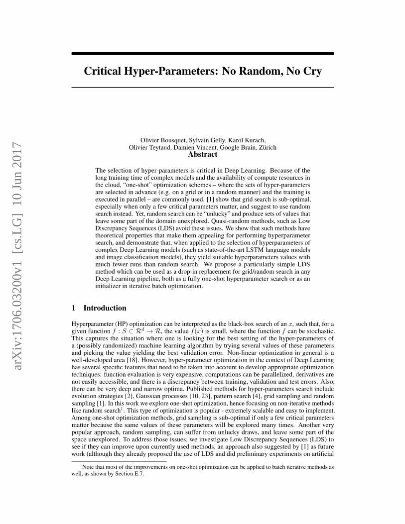
The results can be found in Fig. 2. Using that setup, both LHS and S-SH outperform random onall considered metrics, and for all budgets. LHS outperforms S-SH for small budgets (<11 valuesexplored), while S-SH is best for larger budgets.

2PTB and Enwik8 have systematic differences between the distributions of the train and the validation/testparts, because it is split in the order of the text. That can create systematic biases when an algorithm is moreheavily tuned on the validation set.

6

budget budget∈ budget All budgets< 11 {11, . . . , 28} > 28)

S-SH win rate 0.529± 0.04 0.638± 0.03 0.513%± 0.03 0.569±0.03S-SH speed-up +12.3% +76.6% +5.3% +32%

S-SH bit-per-byte / -1.1% / -0.41%LHS win rate 0.686± 0.06 0.546± 0.04 0.50± 0.07 0.555±0.05LHS speed-up +118% +20% +0% +24.7%

LHS bit-per-byte / -0.08% / -0.48%

Figure 2: Experiments on real-world language modeling, depending on the budget: we providefrequencies at which S-SH (resp. LHS) outperforms random and speedup interpretations. Left:Histogram of budgets used for comparing LHS, S-SH and Random. Right: Winning rate of S-SHand LHS compared to random, on language modeling tasks (PTB, UBPTB, MiniWiki) with variousbudgets.

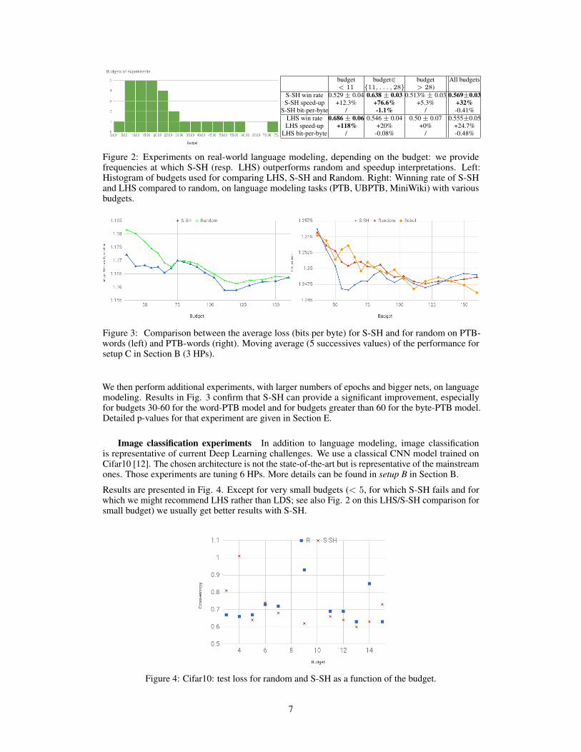
Figure 3: Comparison between the average loss (bits per byte) for S-SH and for random on PTB-words (left) and PTB-words (right). Moving average (5 successives values) of the performance forsetup C in Section B (3 HPs).

We then perform additional experiments, with larger numbers of epochs and bigger nets, on languagemodeling. Results in Fig. 3 confirm that S-SH can provide a significant improvement, especiallyfor budgets 30-60 for the word-PTB model and for budgets greater than 60 for the byte-PTB model.Detailed p-values for that experiment are given in Section E.

Image classification experiments In addition to language modeling, image classificationis representative of current Deep Learning challenges. We use a classical CNN model trained onCifar10 [12]. The chosen architecture is not the state-of-the-art but is representative of the mainstreamones. Those experiments are tuning 6 HPs. More details can be found in setup B in Section B.

Results are presented in Fig. 4. Except for very small budgets (< 5, for which S-SH fails and forwhich we might recommend LHS rather than LDS; see also Fig. 2 on this LHS/S-SH comparison forsmall budget) we usually get better results with S-SH.

Figure 4: Cifar10: test loss for random and S-SH as a function of the budget.

7

Dimension 12Rastrigin Sphere Ellip. Styb. Beale Branin 6Hump

1 batchPessimistic F. 1.00 1.05 1.03 1.00 0.98 1.83 1.18Random init. 1.02 1.30 1.47 1.00 1.07 1.22 1.31

LHS 1.00 1.04 1.09 0.99 0.99 1.72 1.173 batches

Pessimistic F. 1.01 1.06 1.26 1.00 0.83 1.20 0.91Random init. 1.02 1.21 1.20 1.00 0.84 1.08 0.90

LHS 1.03 0.99 1.17 1.00 0.93 1.16 0.995 batches

Pessimistic F. 0.98 1.30 1.47 1.00 1.25 0.89 0.97Random init. 1.01 1.54 1.29 1.00 1.12 0.67 0.83

LHS 0.98 1.44 1.17 1.00 1.34 1.01 1.03

Dimension 2Rastrigin Sphere Ellip. Styb. Beale Branin 6Hump

1 batchPessimistic F. 0.96 1.14 0.95 0.90 0.81 0.95 1.22Random init. 1.01 1.24 1.43 0.95 1.14 0.88 1.13

LHS 1.02 1.17 1.04 0.91 0.84 1.01 1.253 batches

Pessimistic F. 1.12 1.38 1.24 0.03 0.82 1.47 .88Random init. 1.07 0.83 1.00 0.41 0.89 3.14 1.38

LHS 1.01 1.45 1.48 0.06 0.73 0.78 1.195 batches

Pessimistic F. 0.93 1.27 1.10 0.71 1.94 1.61 0.68Random init. 1.01 1.08 1.09 0.58 5.01 1.60 1.14

LHS 1.05 2.09 0.33 0.87 2.56 1.62 0.63

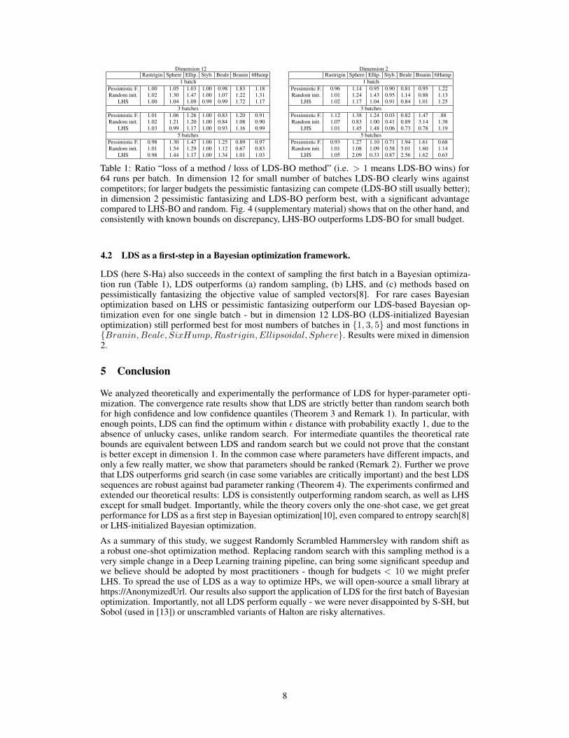
Table 1: Ratio “loss of a method / loss of LDS-BO method” (i.e. > 1 means LDS-BO wins) for64 runs per batch. In dimension 12 for small number of batches LDS-BO clearly wins againstcompetitors; for larger budgets the pessimistic fantasizing can compete (LDS-BO still usually better);in dimension 2 pessimistic fantasizing and LDS-BO perform best, with a significant advantagecompared to LHS-BO and random. Fig. 4 (supplementary material) shows that on the other hand, andconsistently with known bounds on discrepancy, LHS-BO outperforms LDS-BO for small budget.

4.2 LDS as a first-step in a Bayesian optimization framework.

LDS (here S-Ha) also succeeds in the context of sampling the first batch in a Bayesian optimiza-tion run (Table 1), LDS outperforms (a) random sampling, (b) LHS, and (c) methods based onpessimistically fantasizing the objective value of sampled vectors[8]. For rare cases Bayesianoptimization based on LHS or pessimistic fantasizing outperform our LDS-based Bayesian op-timization even for one single batch - but in dimension 12 LDS-BO (LDS-initialized Bayesianoptimization) still performed best for most numbers of batches in {1, 3, 5} and most functions in{Branin,Beale, SixHump,Rastrigin,Ellipsoidal, Sphere}. Results were mixed in dimension2.

5 Conclusion

We analyzed theoretically and experimentally the performance of LDS for hyper-parameter opti-mization. The convergence rate results show that LDS are strictly better than random search bothfor high confidence and low confidence quantiles (Theorem 3 and Remark 1). In particular, withenough points, LDS can find the optimum within ε distance with probability exactly 1, due to theabsence of unlucky cases, unlike random search. For intermediate quantiles the theoretical ratebounds are equivalent between LDS and random search but we could not prove that the constantis better except in dimension 1. In the common case where parameters have different impacts, andonly a few really matter, we show that parameters should be ranked (Remark 2). Further we provethat LDS outperforms grid search (in case some variables are critically important) and the best LDSsequences are robust against bad parameter ranking (Theorem 4). The experiments confirmed andextended our theoretical results: LDS is consistently outperforming random search, as well as LHSexcept for small budget. Importantly, while the theory covers only the one-shot case, we get greatperformance for LDS as a first step in Bayesian optimization[10], even compared to entropy search[8]or LHS-initialized Bayesian optimization.

As a summary of this study, we suggest Randomly Scrambled Hammersley with random shift asa robust one-shot optimization method. Replacing random search with this sampling method is avery simple change in a Deep Learning training pipeline, can bring some significant speedup andwe believe should be adopted by most practitioners - though for budgets < 10 we might preferLHS. To spread the use of LDS as a way to optimize HPs, we will open-source a small library athttps://AnonymizedUrl. Our results also support the application of LDS for the first batch of Bayesianoptimization. Importantly, not all LDS perform equally - we were never disappointed by S-SH, butSobol (used in [13]) or unscrambled variants of Halton are risky alternatives.

8

References

[1] J. Bergstra and Y. Bengio. Random search for hyper-parameter optimization. J. Mach. Learn.Res., 13:281–305, Feb. 2012.

[2] H. Beyer. The theory of evolution strategies. Natural computing series. Springer, Berlin, 2001.

[3] P. Bratley and B. L. Fox. Algorithm 659: Implementing Sobol’s quasirandom sequence generator.ACM Trans. Math. Softw., 14(1):88–100, Mar. 1988.

[4] A. R. Conn, K. Scheinberg, and L. N. Vicente. Introduction to Derivative-Free Optimization.Society for Industrial and Applied Mathematics, Philadelphia, PA, USA, 2009.

[5] T. Domhan, J. T. Springenberg, and F. Hutter. Speeding up automatic hyperparameter optimiza-tion of deep neural networks by extrapolation of learning curves. In Proceedings of the 24thInternational Conference on Artificial Intelligence, IJCAI’15, pages 3460–3468. AAAI Press,2015.

[6] V. Eglajs and P. Audze. New approach to the design of multifactor experiments. Problems ofDynamics and Strengths, 35:104–107, 1977.

[7] J. H. Halton. Algorithm 247: Radical-inverse quasi-random point sequence. Commun. ACM,7(12):701–702, Dec. 1964.

[8] P. Hennig and C. J. Schuler. Entropy search for information-efficient global optimization. CoRR,abs/1112.1217, 2011.

[9] M. Hutter. 50000 euros prize for compressing human knowledge. http: // prize. hutter1.net/ , 2006.

[10] D. R. Jones, M. Schonlau, and W. J. Welch. Efficient global optimization of expensive black-boxfunctions. J. of Global Optimization, 13(4):455–492, Dec. 1998.

[11] Z. S. Karnin, T. Koren, and O. Somekh. Almost Optimal Exploration in Multi-Armed Bandits.In Proceedings of the 30th International Conference on Machine Learning, Cycle 3, volume 28of JMLR Proceedings, pages 1238–1246. JMLR.org, 2013.

[12] A. Krizhevsky, V. Nair, and G. Hinton. Cifar-10 (canadian institute for advanced research).2009.

[13] M. J. Kusner, J. R. Gardner, R. Garnett, and K. Q. Weinberger. Differentially private bayesianoptimization. In F. R. Bach and D. M. Blei, editors, Proceedings of the 32nd InternationalConference on Machine Learning, ICML 2015, Lille, France, 6-11 July 2015, volume 37 ofJMLR Workshop and Conference Proceedings, pages 918–927. JMLR.org, 2015.

[14] L. Li, K. G. Jamieson, G. DeSalvo, A. Rostamizadeh, and A. Talwalkar. Efficient hyperparameteroptimization and infinitely many armed bandits. CoRR, abs/1603.06560, 2016.

[15] M. P. Marcus, M. A. Marcinkiewicz, and B. Santorini. Building a large annotated corpus ofenglish: The penn treebank. Comput. Linguist., 19(2):313–330, June 1993.

[16] M. D. McKay, R. J. Beckman, and W. J. Conover. A comparison of three methods for selectingvalues of input variables in the analysis of output from a computer code. Technometrics,42(1):55–61, Feb. 2000.

[17] G. Rote and R. F. Tichy. Quasi-monte-carlo methods and the dispersion of point sequences.Math. Comput. Model., 23(8-9):9–23, Apr. 1996.

[18] A. Ruszczynski. Nonlinear Optimization. Princeton University Press, Princeton, NJ, USA,2006.

[19] I. Sobol. Uniformly distributed sequences with an additional uniform property. U.S.S.R. Comput.Maths. Math. Phys., 16:236–242, 1976.

[20] A. Sukharev. Optimal strategies of the search for an extremum. USSR Computational Mathe-matics and Mathematical Physics, 11(4):119 – 137, 1971.

[21] B. Tang. Orthogonal array-based latin hypercubes. Journal of the American Statistical Associa-tion, 88:1392–1397, 1993.

[22] B. Tuffin. On the use of low discrepancy sequences in monte carlo methods. Monte CarloMethods and Applications, 2(4):295–320, 1996.

9

[23] J. Villemonteix, E. Vazquez, and E. Walter. An informational approach to the global optimizationof expensive-to-evaluate functions. J. of Global Optimization, 44(4):509–534, Aug. 2009.

[24] C. Wang, Q. Duan, W. Gong, A. Ye, Z. Di, and C. Miao. An evaluation of adaptive surrogatemodeling based optimization with two benchmark problems. Environmental Modelling &Software, 60:167 – 179, 2014.

10

Supplementary material — critical hyperparameters: no random, nocry.

A Proofs

Proof [Lemma 2] A ball of radius ε has volume Vdεd, so if v is the volume of a ball, its radiusis (v/Vd)

1/d. If v is the largest volume of a ball not containing any point of S, then the largesthypercube contained in this ball, which has volume v.Kd will also be empty, which shows thatvdisp(S,B) ≤ Kdvdisp(S,H). Finally it is easy to see that the volume dispersion is upper boundedby the discrepancy as it follows from their definition.

Proof [Theorem 2] For Grid this is a known result[20]. For Random, the probability of n randomlypicked balls of radius ε to contain any particular point x∗ is upper bounded by 1 − (1 − V ′dεd)n,

hence this gives an upper bound of(

log 1/δn

)1/dfor n large with respect to log 1/δ.

For the LDS sequences, this follows from combining Lemma 2 with Theorem 1.

Proof [Theorem 4] The projection of Random (resp. Halton) sequences are Random (resp. Halton)sequences. For Hammersley the first coordinate is uniform, so the projection onto I is Hammersley if1 ∈ I or is Halton otherwise. Theorem 2 allows to conclude. The result for Grid is obvious.

B Detailed experiment setups

Setup A Language model with 3 layers of LSTM with 250 units trained for 6 epochs. Inthis setup, we have 5 hyper-parameters: weight init scale [0.02, 1], Adam’s ε parameter [0.001, 2],clipping gradient norm [0.02, 1], learning rate [0.5, 30], dropout keep probability [0.6, 1].

Setup B Image classification model with 3 convolutional layers, with filter size 7x7, max-pooling,stride 1, 512 chanels; then one convolutional layer with filter size 5x5 and 64 chanels; then two fullyconnected layers with 384 and 192 units respectively. We apply stochastic gradient descent withbatch size 64, weight init scale in [1, 30] for feedforward layers and [0.005, 0.03] for convolutionallayers, learning rate [0.00018, 0.002], epoch for starting the learning rate decay [2, 350], learning ratedecay in [0.5, 0.99999] (sampled logarithmically around 1), dropout keep probability in [0.995, 1.].Trained for 30 epochs.

Setup C Language model with 2 stacked LSTM with 650 units, with the following hyper-parameters: learning rate [0.5, 30], gradient clipping [0.02, 1], dropout keep probability [0.6, 1].Model trained for 45 epochs.

C Toy optimization problems

We conducted a set of experiments on multiple toy problems to quickly validate our assumptions.Compared methods are one-shot optimization algorithms based on the following samplings: Random,LHS, Sobol, Hammersley, Halton, S-SH. We loop over dimensions 2, 4, 8, and 16; we checkthree objective functions (l2-norm f(x) = ||x − x∗||, illcond f(x) =

∑di=1(d − i)3(xi − x∗i )2,

reverseIllcond f(x) =∑di=1(1 + i)3(xi − x∗i )2). The budget is n = 37 in all cases. We used

antithetic variables, thanks to mirroring w.r.t the 3 first axes (hence 8 symmetries). Each methodis tested with and without this 3D mirroring. 3D mirroring deals conveniently with multiples of 8;additional points are generated in a pure random manner. x∗ is randomly drawn uniformly in thedomain. Each of these 12 experiments is reproduced 1221 times.

In each of these 12 cases (4 different dimensions × 3 different test functions), on average over the1221 runs, Sobol and Scrambled-Hammersley performed better than Random in terms of simple

11

regret. This validates, on these artificial problems, both Sobol and Scrambled-Hammersley, in termsof one-shot optimization and face to random search, with p-value 0.0002.

Unsurprisingly, for illcond, Halton and Hammersley outperform random, whereas it is the oppositefor reverseIllcond at least in dimension 8 and 16, i.e. it matters to have the most important variablesfirst for these sequences. Scrambled versions (both Halton and Hammersley) resist much better andstill outperform random - this validates scrambling.

Scrambled Hammersley performs best 6 times, scrambled Halton and Hammersley 2 times each,Sobol and Halton once each; none of the 3d mirrored tools ever performed best. This invalidatesmirroring, and confirm the good behavior of scrambled Hammersley.

These intensive toy experiments are in accordance with the known results and our theoretical analysis(Section 3). Based on the results, the randomly shifted Scrambled-Hammersley is our main LDS forthe evaluation on real Deep Learning tasks.

D Artificial datasets

Our artificial datasets are indexed with one string (AN or ANBN or .N or others, detailed below) and4 numbers. For the artificial dataset C, the 4 numbers are the vocabulary size (the number of letters),maximum word size (n or N ), vocabulary growth and depth - unless specified otherwise, vocabularygrowth is 10 and depth is 3. There are also four parameters for ANBN, AN, .N and anbn; but the twolast parameters are different: they are “fixed size” (True for fixed size, False otherwise) and “size gaps”(impact of size gaps equal to True detailed below). For example, artificial(anbn,26,10,0,1) means thatn is randomly drawn between 1 and 10, and that there are size gaps; whereas artificial(anbn,26,10,1,0)means that n is fixed equal to 10 and there is no size gap.

• AN is a artificial dataset with, as word, a single letter randomly drawn (once for eachsequence) and repeated a fixed number of times (same number of times for differentsequences, but different letter). For examples, the first sequence might be “qqqqqq qqqqqqqqqqqq” and the second one “pppppp pppppp pppppp”.

• The “ANBN” testbed is made of words built by concatenating N copies of a given randomlydrawn letter, followed by N copies of another randomly drawn letter. The words are repeateduntil the end of the sequence. For different sequences, we have different letters, but the samenumber N.

• In the “ABNA” dataset, a word is one letter (randomly drawn, termed A), then N copies ofanother letter (randomly drawn and termed B), and then the first letter again.

• We also use the “.N” testbed, where the “language” to be modelled is made of sequences,each of them containing only one word (made of N randomly independently drawn letters)repeated until the end of the sequence. The first sequence might be “bridereix bridereixbridereix” and the second sequence “dunlepale dunlepale dunlepale”.

• We also have “anbn” as a testbed: compared to ANBN, the number of letters vary for eachword in a same sequence, and the letters vary even inside a sequence. The first sequencemight be “aaabbb ddddcccc db”.

• Finally, we use the “C” testbed, in which there are typically 26 letters (i.e. the vocabularysize is 26 unless stated otherwise), words are randomly drawn combinations of lettersand there exists V × 26 words of e.g. 10 (word size) letters; and there exists V 2 × 26groups (we might say “sentences”) of 10 words, where V is the “vocabulary growth”;there are 3 levels (letters, words, groups of words) when the depth is 3. For exampleartificial(C, 26, 10, 7, 3) contains 26 letters, 26×7 words of length 10, and 26×72 groupsof 10 words.

For each sequence of these artificial datasets, the word size N is randomly chosen uniformly between1 and the maximum word size, except when fixed size is 1 - in which case the word size is always themaximum word size.

If size gaps is equal to True, then the test sizes used in test and validation are guaranteed to not havebeen seen in training; 4 word sizes are randomly chosen for valid and for test, and the other 16 areused in training. There are 10 000 training sequences, 1000 validation sequences, 1000 test sequences.

12

Untuned Half-tuned TunedLearning rate [0.001, 3000] [0.1, 200] [0.5, 30]

Max grad. norm [0.002, 100] [0.006, 30] [0.02, 1.0]Weight init scale [0.02, 1] [0.02, 1] [0.02, 1]

Table 2: Range of hyper-parameters.

Figure 5: Language modeling with moderate networks, (x) in Table 3.

Each sequence is made of 50 words, except for C for which a sequence is one group of the maximumlevel.

In all artificial sequences, letters which are not predictable given the type of sequence have a weight0 (i.e. are not taken into account when computing the loss). In all cases, the loss functions are inbits-per-byte.

E Additional experiments

E.1 Robustness speed-up

In addition to the speed-up defined in Section 4.1, we here define a robustness speed-up.

Speed-up was defined as such because (1 + s)/(2 + s) is the frequency at which a random searchwith budget b × (1 + s) wins against a random search with budget b. We can define the speed-upsimilarly when S competes with several (say K) instances of random search with the same budget b:p = (1+s)/(K+1+s). Note that whenK > 1, we could define another type of speed-up: instead ofthe frequency at which S is better than all K independent copies of random search, we can considerthe frequency at which it performs worse than all these K instances. We call it robustness speed-up;this speed-up is positive when the algorithm is robust and avoids bad cases. When ambiguous, werefer to the initial one as optimistic speed-up, otherwise simply speed-up.

E.2 Average speed-ups over many budgets and testbeds: LDS outperforms random in astable manner

We consider tuning three commonly used hyper-parameters ranked in the following way: learningrate, weight init scale, max gradient norm in three different settings – untuned, half-tuned and tuned –which corresponds to some degree of prior on the expected range of those hyper parameters (Table 2).

S-SH performs clearly better than random (Table 3): all statistically significant results are in favor ofS-SH compared to random. In cases in which the speed-up was negative, this was not statisticallysignificant; and we checked, in all cases in which the speed-up was less than +200%, that therobustness speed-up is still positive.

13

Setting Budgets OptimisticRobustnessspeed-up speed-up

Untuned* 5:12 +350%o

(3 HP, 7 epochs)Untuned* 5:15, 17, 19 +237%o

(3 HP, 7 epochs)Untuned* 25:5:145 +12.8 %o +26%

(3 HP, 7 epochs) (x)Half-tuned* 40:10:120 +50.0 %o +25%

(3 HP, 7 epochs)and 140:20:200

Setting Budgets OptimisticRobustnessspeed-up speed-up

Tuned(3 HP, 7 epochs)* 5:47 -51% +28%

Tuned* 48:73 +87% +50%(3 HP, 7 epochs)

Tuned* 20:5:30 +160%o +160%(3 HP, 4 epochs)

Leaky** 10:5:100 +62 % +40%(5 HP, 30 epochs)

PTB Bytes/Words***budget 20 +57% +57%(7 HP, 17 epochs) budget 30 +0% +0%

(36 xps)

Table 3: Performance of Shifted Scrambled-Hammersley versus random search in various setups. *:PTB bytes and words, Toy sequences (see Section D) C, AN, anbn and ABNA, no size gap, no fixedsize, 3 instances of random vs S-SH, 200 units, 11 epochs. **: leaky setup as defined in SectionE.3, toy sequences .N, AN, anbn with 26 letters and max word size 5 (resp. 10), 2 Lstm, 100 units,with size gaps, variable word size, 3 instances of random vs S-SH. ***: learning rate in [0.5, 30],max gradient norm [2e− 3, 1], Adam’s epsilon [0.001, 2], weight init scale [2e− 3, 10], number ofepochs before learning rate decay [5, 15], dropout keep probability [0.2, 1], 17 epochs, 2 LSTM with650 units, S-SH vs one instance of random. o denote p-values < 0.05; there are cases in which thespeed-up was negative but these cases are not statistically significant; and when the speed-up was lessthan +200% we also checked the robustness speed-up and it was positive in all cases - this illustratesthe robustness property emphasized in Section 3. (x): Fig. 5 suggests a speed-up > 100% for budget' 20− 70 decreasing to zero for large budget.

E.3 Results on toy language modeling problems with additional model hyper-parameters.

We use a modified version of the LSTM cell using 100 leaky state units; each state unit includes 2additional parameters, sampled at initialization time according to a gaussian distribution, whose meanand variance are the 2 additional HPs of the model. Whereas we use, in all experiments (includingthe present ones), learning rate and gradient clipping norm as the two first parameters, a posteriorianalysis shows that the important parameters are these two specific parameters and therefore ourprior (on the ranking of HP) was wrong - this is a common scenario where we do not have any prioron the relative importance of the hyper-parameters. The model was trained on 6 of the artificialdatasets described in Appendix D, namely toy(.N26,5,0,1), toy(.N,26,10,0,1), toy(AN,26,5,0,1),toy(AN,26,10,0,1), toy(anbn,26,5,0,1), toy(anbn,26,10,0,1). We use learning rate ∈ [5, 100], weightinit scale ∈ [0.05, 1], max gradient norm ∈ [0.05, 1], and the two new parameters (mean/std) arerespectively ∈ [−9, 9] and ∈ [0.01, 10]. We check budget 10, 15, 20, 25, . . . , 100. Fig. 6 shows therank of S-SH, among S-SH and 3 instances of random search; this rank is between 1 and 4; afternormalization to [0, 1] we get 0.404± 0.097, 0.456 ± 0.084, 0.281± 0.084, 0.491±0.080, 0.544±0.092, 0.316± 0.081 on these 6 tasks respectively; all but one are in favor of S-SH (i.e. rank < 0.5),2 are statistically significant, and when agregating over all these runs we get an average rank 0.415 at≥ 3 standard deviations from .5, hence clearly significant.

E.4 Other sampling algorithms: S-SH performs best

E.4.1 Validating scrambling/Hammersley on PTB: not all LDS are equivalent

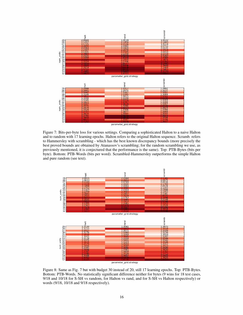
Fig. 7 compares pure random, Halton, and scrambled Halton on PTB-Bytes and PTB-Words. Thesetting is as follows: 7 HPs (dropout keep probability in [0.2, 1], learning rate in [0.05, 300], gradientclipping norm in [0.002, 1], Adam’s epsilon parameter in [0.001, 2], weight initialization scale in[0.002, 10], epoch index for starting the exponential decay of learning rate in [5, 15], learning ratedecay in [0.1, 1]); 17 training epochs, 2 stacked LSTM; we perform experiments for a number ofunits ranging from 12 to 29. The budget for the randomly drawn HPs is 20. Overall, there are36 comparisons (18 on PTB-Bytes, corresponding to 18 different numbers of units, and 18 onPTB-Words);

• Scrambled-Hammersley outperforms Halton 25 times (p-value 0.036);• Scrambled-Hammersley outperforms random 22 times (p-value 0.12);• Halton outperforms random 19 times (p-value 0.43).

14

Figure 6: Rank of S-SH among S-SH and 3 random instances, normalized to [0, 1], on toy languagemodelling testbeds and with leaky LSTM; < 0.5 in most cases i.e. success for S-SH. Points aremoving averages over 4 independent successive budgets hence points 4 values apart are independent.This corresponds to an overall speed-up of +62%, i.e. we get with 50 runs the same best performanceas random with 81 runs.

The experiment was reproduced a second time, with budget = 30 random tries for the HPs. Resultsare presented in Fig. 8 - no statistically significant improvement.

E.5 Robustness vs peak performance

We have seen in Section E.2 that S-SH was always beneficial in terms of robustness; and most oftenin terms of peak performance (optimistic speed-up). We develop this point by performing additionalexperiments. We prefer challenges, so we focus on the so-called tuned-setting in which our results inSection E.2 were least positive for S-SH. We performed experiments with many different values ofthe budget (number of HPs vectors sampled) and tested if S-SH performs better than random in bothlow budget regime (≤ 48) and large budget > 48). Each budget from 5 to 73 was tested. For largebudget regime, S-SH performed excellently, both in terms of best performance (speed-up +87%,p-value 0.09) and worst performance (robustness speed-up +50%, p-value 0.18). For budget ≤ 48,random was performing better than S-SH for the optimistic speed-up (−51%, p-value 0.18); butworse than S-SH for the robustness speed-up (+28%, p-value 0.09). Importantly, this section focuseson the only setting in which S-SH was not beneficial in our diverse experiments (Section E.2); wehave, on purpose, developped precisely the case in which things were going wrong in order to clarifyto which extent replacing random by S-SH can be detrimental.

E.6 Performance as a function of the number of epochs

We consider the untuned setting, on the same 6 problems as (*) in Fig. 3. We have a number ofepochs ranging from 7 to 36, and we consider moving averages of the ranks over the 6 datasets and 4successive numbers of epochs. Fig. 9 presents the impact of the number of epochs; S-SH performsbest overall.

E.7 Results as an initialization for GP

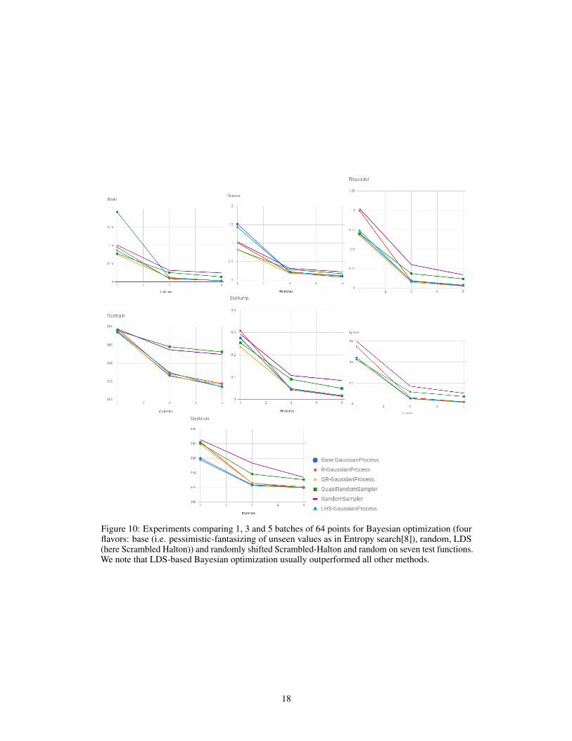
In this section we leave the one-shot setting; we consider several batches, and a Gaussian processes(GP) based Bayesian optimization. Results in [24] already advocated LDS for the initialization ofGP, pointing out that this outperforms Latin Hypercube Sampling; in the present section, we confirmthose results in the case of deep learning and show that we also outperform typical pessimisticfantasizing as used in batch entropy search. The pessimistic fantasizing method for GP is basedon (i) for the first point of a batch, use optimistic estimates on the value as a criterion for selectingcandidates (ii) for the next points in the same batch, fantasizing the values of the previous points inthe current batch in a pessimistic manner; and apply the same criterion as above, assuming thesepessimistic values for previous values of the batch. For the first batch, this leads to regular patterns as

15

Figure 7: Bits-per-byte loss for various settings. Comparing a sophisticated Halton to a naive Haltonand to random with 17 learning epochs. Halton refers to the original Halton sequence. Scramb. refersto Hammersley with scrambling - which has the best known discrepancy bounds (more precisely thebest proved bounds are obtained by Atanassov’s scrambling; for the random scrambling we use, aspreviously mentioned, it is conjectured that the performance is the same). Top: PTB-Bytes (bits perbyte). Bottom: PTB-Words (bits per word). Scrambled-Hammersley outperforms the simple Haltonand pure random (see text).

Figure 8: Same as Fig. 7 but with budget 30 instead of 20, still 17 learning epochs. Top: PTB-Bytes.Bottom: PTB-Words. No statistically significant difference neither for bytes (9 wins for 18 test cases,9/18 and 10/18 for S-SH vs random, for Halton vs rand, and for S-SH vs Halton respectively) orwords (9/18, 10/18 and 9/18 respectively).

16

Figure 9: Untuned setting; rank of each method among 5 methods (3 instances of random, plus Soboland Scrambled-Hammersley), averaged over 6 datasets and 4 successive numbers of epochs (i.e. eachpoint is the average of 24 results and results 3 points apart are independent). This figure correspondsto a budget of 20 vectors of HPs; Scrambled Hammersley outperforms random; Sobol did not provideconvincing results. We also tested a budget 10 and did not get any clear difference among methods.

in grids. We keep the same method for further iterations but replace this first batch by (a) randomsampling (b) low-discrepancy sampling. Results are presented in Fig. 10. We randomly translate theoptimum in the domain but do not rotate the space of functions - which would destroy the concept ofcritical variables. We consider artificial test functions, namely Sphere, Ellipsoid, Branin, Rastrigin,Six-Hump, Styblinski, Beale. We work in dimension 12, with 64 vectors of HPs per batch. Weaverage results over 750, 100 and 50 runs for 1, 3 and 5 batches respectively.

17

Figure 10: Experiments comparing 1, 3 and 5 batches of 64 points for Bayesian optimization (fourflavors: base (i.e. pessimistic-fantasizing of unseen values as in Entropy search[8]), random, LDS(here Scrambled Halton)) and randomly shifted Scrambled-Halton and random on seven test functions.We note that LDS-based Bayesian optimization usually outperformed all other methods.

18

Dimension 12, budget 4

Dimension 12, budget 16

Table 4: Experiments with lower budget, in which case LHS (which has excellent discrepancy forlow budget) performs well. Ratio “loss of a method / loss of LHS-BO method” (i.e. > 1 meansLHS-BO wins) in dimension 12. We see that LHS-BO outperforms LDS-BO for the small budget 4(i.e. most values are > 1). For budget 16, pessimistic fantasizing can compete. BO with randomizedinitialization is always weak compared to LHS-BO.

19