New York State Energy Research and Development Authority

Critical Loads for Air Pollution:Measuring the Risks to Ecosystems

Energyfor

Primer May 2014

Report Number 14-24

NYSERDA’s Promise to New Yorkers: NYSERDA provides resources, expertise, and objective information so New Yorkers can make confident, informed energy decisions.

Mission Statement:Advance innovative energy solutions in ways that improve New York’s economy and environment.

Vision Statement:Serve as a catalyst—advancing energy innovation and technology, transforming New York’s economy, empowering people to choose clean and efficient energy as part of their everyday lives.

Core Values:Objectivity, integrity, public service, partnership, and innovation.

PortfoliosNYSERDA programs are organized into five portfolios, each representing a complementary group of offerings with common areas of energy-related focus and objectives.

Energy Efficiency and Renewable Energy Deployment

Helping New York State to achieve its aggressive energy efficiency and renewable energy goals – including programs to motivate increased efficiency in energy consumption by consumers (residential, commercial, municipal, institutional, industrial, and transportation), to increase production by renewable power suppliers, to support market transformation, and to provide financing.

Energy Technology Innovation and Business Development

Helping to stimulate a vibrant innovation ecosystem and a clean-energy economy in New York State – including programs to support product research, development, and demonstrations; clean-energy business development; and the knowledge-based community at the Saratoga Technology + Energy Park® (STEP®).

Energy Education and Workforce Development

Helping to build a generation of New Yorkers ready to lead and work in a clean energy economy – including consumer behavior, youth education, workforce development, and training programs for existing and emerging technologies.

Energy and the Environment

Helping to assess and mitigate the environmental impacts of energy production and use in New York State – including environmental research and development, regional initiatives to improve environmental sustainability, and West Valley Site Management.

Energy Data, Planning, and Policy

Helping to ensure that New York State policymakers and consumers have objective and reliable information to make informed energy decisions – including State Energy Planning, policy analysis to support the Regional Greenhouse Gas Initiative and other energy initiatives, emergency preparedness, and a range of energy data reporting.

3

Contents

Preface ................................................................................ 5

What are Critical Loads? ...................................................... 6

Nitrogen and Sulfur Emissions ..........................................7

Acidification by Sulfur and Nitrogen .................................... 8

Fertilization by Nitrogen ....................................................... 9

Measuring Nitrogen Impacts .......................................... 10

Empirical Nitrogen Loads ............................................... 11

Mapping Empirical Loads ................................................ 12

Measuring the Impacts of Acidification ......................... 13

Acidification and Weathering ......................................... 14

Modeling Critical Loads For Acidification ..................... 15

Modeling Acidification II: Dynamic Models ................... 16

Using Critical Loads to Assess Ecological Risk ............ 17

Summary and Prospects ................................................ 18

References ...................................................................... 20

Acknowledgements and Credits .................................... 21

This document is a product of the New York State Energy Research and Development Authority (NYSERDA). It was developed by Jerry Jenkins of the Wildlife Conservation Society, in consultation with Timothy Sullivan of E&S Environmental Chemistry. Greg Lampman supervised the project for NYSERDA.

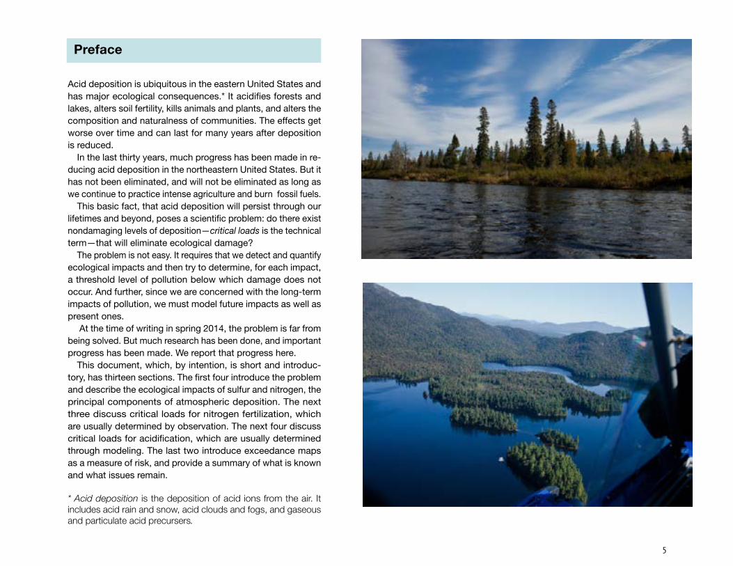
Above, old-growth red spruce near Oswegatchie River, Fine, New York Top right, Pelletier Deadwater, Allagash River, Maine. Lower right, Ampersand Pond, Harrietstown, New York. Cover, Deer Island, Upper Saranac Lake, Santa Clara, New York.

4

5

Preface

Acid deposition is ubiquitous in the eastern United States and has major ecological consequences.* It acidifies forests and lakes, alters soil fertility, kills animals and plants, and alters the composition and naturalness of communities. The effects get worse over time and can last for many years after deposition is reduced.

In the last thirty years, much progress has been made in re-ducing acid deposition in the northeastern United States. But it has not been eliminated, and will not be eliminated as long as we continue to practice intense agriculture and burn fossil fuels.

This basic fact, that acid deposition will persist through our lifetimes and beyond, poses a scientific problem: do there exist nondamaging levels of deposition—critical loads is the technical term—that will eliminate ecological damage?

The problem is not easy. It requires that we detect and quantify ecological impacts and then try to determine, for each impact, a threshold level of pollution below which damage does not occur. And further, since we are concerned with the long-term impacts of pollution, we must model future impacts as well as present ones.

At the time of writing in spring 2014, the problem is far from being solved. But much research has been done, and important progress has been made. We report that progress here.

This document, which, by intention, is short and introduc-tory, has thirteen sections. The first four introduce the problem and describe the ecological impacts of sulfur and nitrogen, the principal components of atmospheric deposition. The next three discuss critical loads for nitrogen fertilization, which are usually determined by observation. The next four discuss critical loads for acidification, which are usually determined through modeling. The last two introduce exceedance maps as a measure of risk, and provide a summary of what is known and what issues remain.

* Acid deposition is the deposition of acid ions from the air. It includes acid rain and snow, acid clouds and fogs, and gaseous and particulate acid precursers.

6

What are Critical Loads?

A critical load is a measure of the ecological impact of air pol-lution. Specifically, it is the maximum continuing load of pollut-ants that a community can tolerate without suffering damage.

A critical load is thus a threshold for damage. Below the criti-cal load there is, in concept, no damage, no matter how long the pollution continues. Above it, there is.

The lower diagram at right shows the key idea. A forest receives nitrogen in rain and snow. Based on observations in many forests, at loads of about 250 equivalents of deposition per hectare per year (eq/ha-yr) the growth and survival of the most sensitive trees begin to change. At loads of about 700 eq/ha-yr, the forest can no longer store all the nitrogen it receives, and nitrate appears in the soil water and is exported to streams and lakes.

Since tree growth and nitrogen loss are key measures of ecosystem function, these values are estimates of the minimum loads at which natural processes become altered. They are thus the critical loads for tree growth and nitrogen loss.

Loads, like these, determined by observation or experiment are called empirical loads. Loads, like those discussed on pages 15 and 16, determined by simulating watershed chemistry, are called modeled loads.

Several things are worth noting at the outset. First, there is no guarantee that a critical load exists. Some biological groups, like grassland plants and forest lichens, are very sensitive to nitrogen, and may show changes at very low rates of deposition. In such groups there may be no clear threshold below which impacts cease, and, hence, no critical load.

Second, critical loads vary depending on who receives the load. Tree growth in forests has one critical nitrogen load. Forest lichens have another, and forest herbs yet another. No single loads describes all groups or the forest as a whole.

And third, the empirical loads just described are short-term estimates of the pollution a community can tolerate. Because the impacts of pollution often increase over time, the long-term load for continuing pollution may be lower.

Above, pollutant loads are measured in units of mass (kilograms) or electrical charge (equivalents) per unit area per time. Here we use charge, which makes it easier to compare different pollutants. Our preferred units are equivalents per hectare per year, written eq/ha-yr, or, for convenience in labeling graphs, hundreds of equivalents per hectare-year, written 100 eq/ha-yr.

Below, two examples of critical loads for nitrogen. Tree growth and survival in northeast-ern forests begin to change at nitrogen loads of around 250 eq/ha-yr. Excess nitrogen starts to appear in surface waters at around 700 eq/ha-yr.

7

Nitrogen and Sulfur Emissions

Four air pollutants—sulfur, nitrogen, ozone, and mercury—have significant effects on the ecology of the United States. Sulfur and nitrogen have had the most study, and we focus on them here.

Sulfur pollution comes largely from a single source, the sulfur in fossil fuels. The largest emitters are boilers in power plants and factories that burn coal and heavy oil. Burning converts sulfur to sulfur oxides, which are then delivered to ecosystems by wet deposition—mist, rain, and snow—and by dry deposition—droplets and particles intercepted by soil, water, or vegetation.

Nitrogen pollution comes from both fossil fuels and agricul-ture. The combustion of fossil fuels converts nitrogen to nitro-gen oxides. Agricultural fertilizers and animal wastes generate nitrogen oxides and ammonia. Once in the atmosphere, the nitrogen oxides are converted to nitric acid, and the ammonia to ammonium. Both are then delivered to ecosystems by wet and dry deposition.

Nitrogen and sulfur emissions built up rapidly as U.S. in-dustry and agriculture intensified after World War II. They peaked sometime in the 1970s and have since been reduced by a combination of legislation (the Clean Air Act of 1970 and its amendments of 1977 and 1990) and federal rule-making authorized by legislation. As a result, the current emissions of sulfur oxides are about a fifth of what they were in 1970, and the emissions of nitrogen oxides about half.

Deposition has decreased accordingly. In 2011, total sulfur and nitrogen deposition at Huntington Forest in the central Adirondacks was about 370 eq/ha-yr, down from over 600 eq/ha-yr in 2003. In southwestern Adirondacks, however, which are nearer the big coal-fired electrical plants in the Ohio Valley, it was roughly twice that.

The decreases have been substantial but they are still de-creases from a large total. The United States still emits over 15 million tons of nitrogen and sulfur oxides per year into the air and suffers significant ecological damage as a result. Data from the U.S. Energy Information Agency, and the Clean Air Status

and Trends Network. Note that nitrogen emissions from farms are not in-cluded in the graph of nitrogen oxide emissions.

8

Acidification by Sulfur and Nitrogen

The nitric and sulfuric acids deposited on ecosystems begin a chemical and biological chain reaction called the acidification cascade. The cascade includes both direct and indirect reactions.

The acids have multiple effects. They are directly toxic to lichens and mosses, and probably some forest herbs as well. They affect many other groups—trees, fungi, invertebrates,birds—indirectly by acidifying the soil. And, as explained in the next section, they affect whole communities by altering nutrient cycling.

Acidified soils store acid ions like hydrogen and lose bases like calcium and magnesium. They also release inorganic alu-minum, which is toxic, into the soil water.

Acidified forest soils are thus base-cation poor, while the wa-ter in their pores is aluminum rich. The limited supply of bases reduces the growth rate, regeneration, and health of forest trees. The high aluminum concentrations in the soil water are toxic to tree roots and their associated fungi.

The loss of bases also impacts forest food chains. Soil inver-tebrates need calcium for exoskeletons and shells. Base-poor soils have fewer soil invertebrates. Fewer soil invertebrates mean less food for forest-floor animals like thrushes and shrews, and so less food for the mesocarnivores like owls and weasels that depend on them.

The water from acidified soils flows into streams and lakes, reducing their pH and acid-neutralizing capacity. The buffering capacity—the ability of the water to resist changes in acidity—can drop to near zero, and leave the lake or stream vulnerable to rapid pH changes. Dissolved organic carbon often decreases, and toxic mercury and inorganic aluminum often increase.

As in the forest, the chemical changes in lakes and streams have biological impacts. Low pH waters are less productive than high-pH ones, with fewer plants and algae and less photosyn-thesis. Food chains are short, and animals grow more slowly. Aluminum-sensitive groups like mayflies or native minnows may be eliminated altogether. Mercury accumulates in fish and can reach dangerously high levels in fish-eating animals like loons and mink.

9

Fertilization by Nitrogen

Nitrogen is an essential nutrient for all animals and plants. In undisturbed ecosystems, nitrogen inputs are often low. Nitrogen cycles from the soil to plants, from plants to animals, and then, through fungi and microbes, back to the soil when the plants and animals die and decay.

In undisturbed communities, nitrogen is often in short supply, and nitrogen cycling is tight. The plants in these communities are adapted to low nitrogen levels and can use it quite efficiently. Tis-sue nitrogen levels are low, and there is little biologically available nitrogen in the soil or in surface water.

Nitrogen deposition introduces excess nitrogen in biologically useful forms, causing a series of changes called the fertilization cascade. The first changes are physiological. Plants take up the extra nitrogen. Some use it for growth. Others, including many low-nitrogen specialists, store it in their tissues, where it may cause physiological damage. Membrane calcium may be lost, and cold damage may become more common. Fine root biomass decreases and the diversity of the symbiotic fungal communities associated with roots decreases.

The physiological changes lead to ecological ones. Nitrogen-demanding species, often alien, out-compete the native low-nitrogen specialists. Rare species are lost and the number of native species declines. Nitrogen-rich plants attract pathogens and herbivores, and disease and defoliation become more common.

All of these changes compromise the tightness of the nitrogen cycling. For a while the community stores the excess nitrogen in biomass and soil. But eventually a limit is reached, and nitrogen begins to leak into groundwater and migrate to streams and lakes.

Once it gets there, a similar fertilization cycle begins in the waterbody. If a lake or stream is nitrogen-limited, the excess nitrogen will stimulate the growth of algae and alien species. Productivity increases, transparency and dissolved oxygen decrease, less-competitive species are eliminated, and overall diversity decreases.

10

Measuring Nitrogen Impacts

The simplest way of determining critical loads is to compare how actual communities are responding to pollution. If you can find the threshold load at which impacts begin, that is the critical load.

To do this, you need to observe the same community under dif-ferent pollutant loads. This can be done either by studying sites along a gradient of differing pollutant loads or by varying the load-ing experimentally.

Mark Fenn and his collaborators studied the response of lichens along a pollution gradient in California. At pristine sites where de-position was near zero, the lichen communities were dominated by low-nitrogen species, and the tissues of the wolf lichen, Letharia, contained at most 1% nitrogen. As nitrogen deposition increased, the communities shifted away from low-nitrogen species and the wolf lichen tissue nitrogen increased. They estimated that the changes began at a load of about 250 eq N/ha-yr.

Paul Schaberg and his collaborators used an experimental ap-proach to determine whether nitrogen deposition affects the cold tolerance of red spruce. They established sample plots on Mt. Ascutney, Vermont, treated them for 12 years with four different loads of nitrogen, and measured the cold tolerance, winter injury, and membrane function of the spruce in the plots.

Their results show that the spruce on the treated plots had more winter injury, less cold tolerance, less membrane calcium and more electrolyte leakage than the spruce on the control plots. But because there was appreciable background nitrogen deposition at their study site, they had no controls with zero load and so could not identify the critical load at which cold tolerance starts to decrease.

Gradient and experimental studies are complimentary, and each has strengths and weaknesses. Schaberg’s study showed clearly that added nitrogen changes the cold tolerance of spruce but could not identify the threshold where the change begins. Fenn’s study identified the critical nitrogen load at which lichen communities start to change but, because other pollutants vary with nitrogen, could not prove that the impacts were caused by nitrogen.

Top graph from Fenn, 2008, copyright Elsevier Ltd., used with permission.Lower graphs from Schaberg et al, 2002, copyright National Research Coun-cil of Canada, used with permission. Schaberg’s study site had a background nitrogen deposition of 450 eq/ha-yr at all plots, so even the control plots were receiving significant amounts of nitrogen.

11

Empirical Nitrogen Loads

Critical loads determined from field studies are called empiri-cal loads. They are generally specific to a particular biological group in a particular natural community. Thus the critical load for lichens will not, in general, be the same as the critical load for shrubs or trees, and the critical load for herbs in grasslands may be different from that for herbs in forests.

None the less, as more studies have been done, some broad patterns have emerged. Our first look at these patterns came in 2011 when Linda Pardo and 22 collaborators did a continental-scale synthesis of American nitrogen studies.

Their synthesis used 50 studies from 3,200 field sites and estimated critical loads for eight different kinds of impacts in 15 different biomes. They assumed, conservatively, that a small change observed in a short-term study may grow larger over time and so defined the critical load as the lowest load that produced a measurable biological impact.

The studies they used are wide ranging. They included lichens and shrubs in arctic tundra, bryophytes in bogs, grasses in prairies, mycorrhizal fungi in Pacific Coast forests, and invasive grass species in deserts. Their results are clearly preliminary —it will take more studies to fill the gaps and increase the reliability of the results—but are consistent with much work from Europe and elsewhere, and suggest three important generalizations.

First, nitrogen fertilization is one of the most pervasive forms of air pollution. It affects almost every biome in the United States and Europe and likely many in Africa and Asia as well.

Second, almost every biome shows changes at nitrogen loads under 1,000 eq/ha-yr, and many show changes at levels under 500 eq/ha-yr.

And third, the sensitivity of communities and biological groups differs greatly. For sensitive communities, like tundra, grasslands, and mountain lakes and forests, and sensitive groups, like fungi, diatoms, and grassland herbs, the critical loads may be close to zero. For the most sensitive of these, there may be no nonzero loads that do not favor some species and harm others. Based on Pardo, 2011a, Original figure copyright Ecological Society of America

and used with permission. The numbers following the colored bars are the number of studies. A zero means the value is based on studies from a different region.

12

Mapping Empirical Loads

Because every community contains biological groups with differ-ent sensitivities, there is no single critical load at which the whole community starts to change. Instead, change is incremental, with the most sensitive groups changing first, then those of intermediate sensitivity, and finally those that are least sensitive.

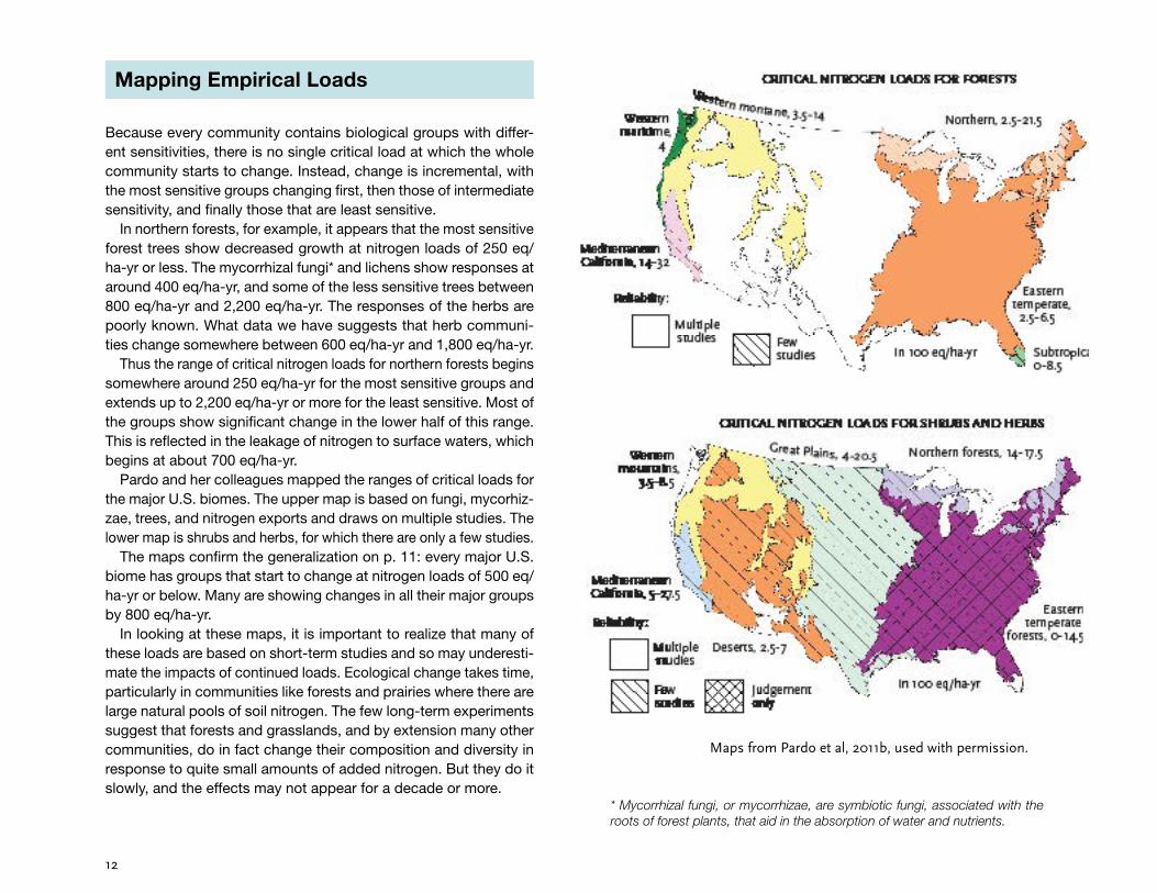
In northern forests, for example, it appears that the most sensitive forest trees show decreased growth at nitrogen loads of 250 eq/ha-yr or less. The mycorrhizal fungi* and lichens show responses at around 400 eq/ha-yr, and some of the less sensitive trees between 800 eq/ha-yr and 2,200 eq/ha-yr. The responses of the herbs are poorly known. What data we have suggests that herb communi-ties change somewhere between 600 eq/ha-yr and 1,800 eq/ha-yr.

Thus the range of critical nitrogen loads for northern forests begins somewhere around 250 eq/ha-yr for the most sensitive groups and extends up to 2,200 eq/ha-yr or more for the least sensitive. Most of the groups show significant change in the lower half of this range. This is reflected in the leakage of nitrogen to surface waters, which begins at about 700 eq/ha-yr.

Pardo and her colleagues mapped the ranges of critical loads for the major U.S. biomes. The upper map is based on fungi, mycorhiz-zae, trees, and nitrogen exports and draws on multiple studies. The lower map is shrubs and herbs, for which there are only a few studies.

The maps confirm the generalization on p. 11: every major U.S. biome has groups that start to change at nitrogen loads of 500 eq/ha-yr or below. Many are showing changes in all their major groups by 800 eq/ha-yr.

In looking at these maps, it is important to realize that many of these loads are based on short-term studies and so may underesti-mate the impacts of continued loads. Ecological change takes time, particularly in communities like forests and prairies where there are large natural pools of soil nitrogen. The few long-term experiments suggest that forests and grasslands, and by extension many other communities, do in fact change their composition and diversity in response to quite small amounts of added nitrogen. But they do it slowly, and the effects may not appear for a decade or more.

Maps from Pardo et al, 2011b, used with permission.

* Mycorrhizal fungi, or mycorrhizae, are symbiotic fungi, associated with the roots of forest plants, that aid in the absorption of water and nutrients.

13

Measuring the Impacts of Acidification

Acidification, as explained on p. 8, is caused by both sulfur and nitrogen, and affects both surface waters and forests.

Its effects on lakes and streams have been extensively researched. Acidification decreases pH and increases toxic aluminum. These cause biological stress and species begin to drop out. Species richness drops, and the overall abundance of animals and plants declines.

The process, like the nitrogen fertilization of a forest, is incre-mental, with different species dropping out at different acidities. None the less, there seems to be a range between pH 6.0 and 5.0 where many species begin to be impacted by acidity. At pH 5.5, for example, only two of the twenty-five northeastern fish in the table at right show the impacts of acid. At pH 5.0, twelve do.

Much the same happens with other groups. As a result, pH is considered a master variable in lake biology, and there is a general consensus in the literature that most lakes will show the impacts of acidity by pH 5.5.

Forests are different, and there is no similar consensus about measuring forest acidification. The problem is that the effects of forest acidification are slower and less direct. Forest acidification involves a gradual loss of soil bases and a gradual increase in free aluminum in the soil solution. Because these processes take time, and because trees are long lived and respond slowly to environmental changes, the biological changes are hard to measure.

Despite these difficulties, there is a growing body of research that suggests that at least some trees are sensitive to acidifica-tion and that, as soil bases are lost, their health declines and their ability to regenerate decreases.

Following this reasoning, many researchers are using the base saturation (the percentage of soil binding sites occupied by bases) as a measure of forest acidification. While we still have no graphs showing how many species are stressed at different levels of base saturation, there is evidence that sensitive spe-cies like sugar maple start to decline at base saturations under 20%, and that other species may decline at base saturations under 10%.

Redrawn from Baker and Christensen, 2009. Copyright Springer Science and Business Media, and used with permission.

14

Acidification and Weathering

The empirical loads for nitrogen described on pp. 11-12 were derived from dose-response relations between nitrogen loads and biological impacts. So much nitrogen per year on one of Fenn’s western forests meant so much nitrogen in lichen tissue and so much excess nitrogen flowing out in the streams.

Acidification, unfortunately, is more complicated. The rate of acidification depends on the balance between the input of acids, which come largely from deposition, and the input of bases, which come largely from the weathering of soil minerals. As shown in the diagrams, two watersheds with the same deposition but different soils can have different weathering rates and differ-ent acid-base balances. The one with the high weathering rate will have a higher soil base saturation and surface water with a higher acid-neutralizing capacity. It will be able to neutralize more incoming acid and so will have a higher critical load.

The result is that there are no simple dose-response relations between acid loads and soil or water chemistry. Two adjacent watersheds may receive the same acid load but have quite differ-ent base saturations and pHs, and hence different critical loads.

This variability, resulting from differences in soil depths and weathering rates, changes the determination of critical loads in two important ways. The first is that critical loads for acidification have to be determined separately for each watershed. This is usually done by modeling the chemical balance between inputs and outputs (pp. 15-16). Such modeling is difficult because weathering rates are poorly known, and because the modelers have to determine what chemical values are biologically mean-ingful to model. But it is also powerful, because it can predict critical loads over large areas.

The second is that critical loads for acidification turn out to vary greatly from watershed to watershed. Some watersheds with high weathering rates may never be acidified at current loads. Others may remain impacted even if current loads are reduced to zero.

As a result, critical loads, which started as simple numbers, have become something more complex. They are now estimates of risk, showing how many watersheds are safe at a given load.

Two contrasting watersheds, with the same deposition but dif-ferent soils and weathering rates. A full accounting would also involve rates of acid and base removal through denitrification, immobilization, and harvesting, as in the top diagram on p. 15, but these are usually small compared to deposition and weathering terms.

15

Modeling Critical Loads For Acidification

Critical loads modeling is widely used in Europe and Canada, and becoming so in the United States. The goal is to escape from the messiness of empirical studies and create a simple picture of acidification over wide areas.

To do this the models usually make two major simplifications. They replace watersheds with boxes, and they replace biology with chemistry.

Replacing watersheds with boxes means ignoring spatial variation and using average values. Each watershed is assigned, a uniform elevation, soil depth, and chemistry, and the variation of these quantities within the watershed is ignored.

Replacing biology with chemistry means ignoring the vari-ability in biological responses and assuming ecological damage starts when some chemical threshold—say an acid-neutralizing capacity of 50 µeq/l or a base saturation of 20%—is crossed. The threshold values are usually assumed to be the same in all the watersheds being modeled, regardless of the local biology.

With these simplifications, it is possible to use relatively simple models, called simple mass-balance models, to map critical loads.

The models treat each watershed as a single box, into and out of which ions flow at a steady rate. The models are tested with increasing amounts of deposition until they reach a load which produces the chosen threshold value. This deposition rate is the modeled critical load.

The map, by Steve McNulty and his collaborators, shows the results from one such model. The critical loads for acidification are lowest on the relatively thin and depleted soils of the northern Appalachians, Lake States and the sandy coastal plain. They are higher in the base-rich southern and western mountains but low again, locally, where the bedrock is low in bases.

These results correspond fairly well to what we know about lake and stream chemistry and suggest that the models, for all their simplifications, are capturing important patterns of ecological sensitivity.

From McNulty et al., 2007, copyright Elsevier Ltd. and used with permission.

16Maps above and on p. 17 from Sullivan et al, 2012 Copyright American Geophysical Union, used with permission.

Modeling Acidification II: Dynamic Models

Simple mass-balance models are essentially chemical snapshots, showing watershed chemistry at one moment in time. They assume that the inputs and outputs never vary and that pools of acids and bases in the water shed never change.

Watershed chemistry, however, varies in time. Flows are high and low, pollutant loads change, ions are stored and released, soils are depleted, climate changes. To represent these processes we need to replace snapshots with movies. Dynamic watershed models, like MAGIC and PnET-BGC, which show how a watershed evolves from a given starting point under a given deposition scenario, provide such movies.

Dynamic models are more complicated than static models and require more detailed watershed data. But because they predict future chemistry, they give more realistic assessments of risk than static models. And because they are data-intense and have been tested against long-term data from experimental watersheds, they are thought to be more reliable than simple mass-balance models.

Dynamic models are just starting to be used to model critical loads over large areas. The map at the right, by Tim Sullivan and his collaborators is the first produced for the northeast United States. It shows the sulfur loads which will maintain acid-neutralizing capacities of 50 µeq/l or greater for 90 years in Adirondack lakes.

The most interesting feature, which corresponds well to what we know of the chemistry and biology of these watersheds, is just how variable the critical loads are. Many Adirondack watersheds, especially in the west, have loads under 250 eq/ha-yr. Others, some-times only a few miles away, have loads 1,000 eq/ha-yr or higher.

This variability suggests that we must generalize our notion of critical loads. Instead of a critical load being a boundary below which everything is safe, it is now a function telling us how the percentage of lakes at risk varies with load. At low loads, say 100 eq/ha-yr, almost all the lakes are safe. At the high loads, say 2,000 eq/ha-yr almost none are. In the middle, some are safe and some aren’t.

Thinking of critical loads as risk functions is more complicated but also more realistic. For any given load, some lakes will be safe and some at risk. What we need to know is how many of each there are. The value of the modeling approach is that it can tell us this.

17

Using Critical Loads to Assess Ecological Risk

By themselves, critical loads measure the potential sensitivity of ecosystems but not the actual risks they face. A sensitive eco-system may be at high risk even where the deposition is low; an insensitive one may be safe even when it is high.

To measure risk we need to know how the actual deposition compares to the critical load. To compute this, we may compare the critical load to the actual load, as in the upper diagram, or divide one by the other, as in the lower.

The result is the exceedance, which compares the actual de-position to the deposition at which we believe that impacts begin. A high exceedance means that the deposition greatly exceeds the critical load, and hence ecological damage is likely. A low exeedance means the reverse.

Exceedance is a useful measure because it is synthetic, mean-ing that it combines many details of biology and chemistry, and statistically robust, meaning that it allows conclusions that are independent of the errors in individual critical-load calculations.

Two examples show this. The upper map, from Pardo and her colleagues, shows the parts of the country where the empirical critical nitrogen loads for forests are currently exceeded. The map provides a simple and cogent summary, independent of the details of forest biology and the estimated sensitivities of different forests. All eastern forests, and many western mountain ones, are currently at risk of ecological damage from nitrogen deposition.

The lower map, from Sullivan and his colleagues, shows a great range of local exceedances, comparable to the range of critical loads shown on p. 16. Many watersheds, especially those in the east, seem to be safe at current deposition rates. But many others, especially in the west, show high exceedances and are at risk.

Given the uncertainties of data and modeling, we cannot be certain of the exceedance of any given watershed. But given both the number of high-exceedance watersheds and our independent knowledge of acidification in many of these watersheds, the gen-eral conclusion “a third or more of the Adirondack watersheds for which we have data are currently at risk from lake acidification,” is statistically robust.

18

Summary and Prospects

The science which underlies our understanding of the ecological impacts of pollution is less than forty years old and the use of this science to calculate critical loads less than twenty-five. In this period there have been at least four major accomplishments.

1. We now understand the processes involved in both acidification and fertilization, and have identified biological markers associ-ated with the acidification of lakes and the fertilization of both lakes and forests. Work is proceeding on the biological markers of forest acidification, but they are still poorly known.

2. Preliminary estimates of empirical critical loads for nitrogen fertilization and maps of exceedances have been prepared for all the major biomes of the United States.

3. Simple mass-balance models have now been used to map short-term critical loads and exceedances for acidification for the entire United States.

4. Dynamic models have now been used to predict critical loads for the next hundred years in the Adirondacks, Shenandoah National Park, the southern Appalachian Mountains, and selected watersheds in California, New Hampshire, and Colorado.

These accomplishments come with warnings. The biological data on which the empirical critical loads are based are still sparse. The ability of the computer models to predict the acidification of forest soils has not been adequately validated.

And the accuracy with which exceedance maps can predict where damage is occurring—which is, after all, the reason for computing critical loads—has only been assessed in a few studies.

Warnings notwithstanding, the language of critical loads allows us to synthesize our knowl-edge of the ecological impacts of pollution in a way that was not possible even a few years ago. The key elements in this synthesis are that:

1. Critical loads are not simple numbers, but rather ranges of numbers that describe how the risk of ecological damage varies from the most sensitive sites and species to the least sensitive.

2. Low-nitrogen ecosystems, like most grasslands, northern forests, and wetlands, are very sensitive to nitrogen fertilization. They typically show biological responses before they show chemical ones, and, for their most sensitive species, the critical loads are close to zero.

3. Maps of exceedances suggest that, even with the reductions in emissions that have taken place, large portions of the eastern United States may be suffer-ing ecological damage from sulfur and nitrogen.

These are noteworthy advances in our understanding, and speak to the value of the critical loads approach.

What, then, are the next steps? Clearly, more research. Also more empirical studies, more model-ing, and more testing of model predictions.

Some of this will be geochemical. Someone will need to constrain the uncertainties in weathering rates and figure out whether our current models, which after all, were developed to predict water chemistry, can predict soil chemistry as well.

Much of work, however, will be biological. If the exceedance maps are right, acidification and enrichment are pervasive problems. We will need many more studies—of tree growth rates, of herbs, of eastern mosses and lichens of snails and the thrushes that eat them—before we will really know what the biological effects are, and what chemical thresholds correspond to them.

The latter—the identification of the thresholds that mark the beginning of damaging change—is critically important. All the modeling skill in the world will avail us little without a clear sense of what it is biologically meaningful to model.

The needed research will, of course, take time. But the progress in the last ten years has been impressive. With adequate resources, much more should happen in the next ten.

Osgood River, Brighton, N.Y.

19

Madewaska Pond, Meno, N.Y.

Notes

p. 6 For general discussions of critical loads see Burns, 2008, and Pardo 2011. The nitrogen loads in the illustration are from Thomas, 2011, and Aber, 2003. For the re-sponses of grasslands to low levels of nitrogen, see Bobbink, 2010.

p. 7 Deposition data at http://epa.gov/castnet/javaweb/mapcharts.html. Wet deposition is measured at many sites and is relatively well known. Dry deposition is measured at far fewer sites and is less well known.

p. 8 For book-length treatments of acidification see Jenkins, 2007, and Sullivan, 2000. For a concise summary see Lovett, 2009.

p. 9 For the impacts of nitrogen see Aber, 1989; Baron, 2000; Fenn, 2008; Lovett, 2009; Thomas, 2010; Pardo, 2011; and the literature referenced by these works.

Most biologically-available ni-trogen in terrestrial communities comes from the fixation (conversion to nitrate) of atmospheric nitrogen by bacteria. Nitrogen fixation is limited in northern and upland communities, and so our forests and boreal wetlands are typically low-nitrogen communities.

p. 10 Note that, like many empirical studies, neither Fenn nor Schaberg could determined the threshold for impact with certainty.

p. 11 The figure is based on Figure 8 in Pardo, 2011b, with additional values from her Table 6 added. Note that, in comparison to the hundreds

of studies of nitrogen concentra-tions in surface waters, our total knowledge of the biological impacts of nitrogen in northern forests and tundra comes from fewer than 20 studies. Many groups, like eastern herbs and lichens, have not had detailed studies, and their critical loads had to be inferred from stud-ies in other biomes.

p. 12 From Pardo, 2011b.

p. 13 For the biology of stream and lake acidification, see Jenkins, 2007, Chapter 8, and the refer-ences cited there. No comparable synthesis of the biology of forest acidification seems to be available, but see Bailey, 2005, and Long, 2009, for some recent work. The discussion of base saturation in the last paragraph is drawn from personal communications.

p. 14 The large uncertainties in weathering rates arise from the lack of detailed soil data and influ-ence all modeling of critical loads. Pardo, 1993, concluded that the lack of weathering data “severely limited” the usefulness of simple mass-balance models for comput-ing critical loads for acidification. Duarte, 2012, estimated that 80% of the variance in the critical loads they modeled came from varia-tions in the weathering rate and that critical loads for a single site could differ by as much as ten times depending on the weathering rate they assumed.

p. 15 For other examples of simple mass-balance models see Wat-mough, 2006; Fenn, 2008; and Pardo, 2013.

When simple mass-balance mod-els are used to predict the critical loads for forest acidification, what they are actually doing is predicting some measure of soil chemistry, usually base saturation or base-to-aluminum ratio. It is important to note that, so far as we know, there have been no large-scale validation studies comparing these predictions against measurements.

p. 16 For dynamic modeling of soil acidification using the same dataset, see Sullivan, 2011. For the struc-ture and validation of the MAGIC model, see Cosby, 2001, and for dynamic modeling in Europe, see Hettelingh, 2008. For a comparison of four models applied to the same site, see Tominaga, 2010,

The dynamic models being used to compute critical loads have had extensive development and testing, and their ability, given adequate data

for calibration, to simulate short-term changes in water chemistry seems well established.

Whether they are equally good at predicting the changes in soil chemistry involved in forest acidifica-tion is unknown, because there are almost no time-series of soil data to test them against. And finally, their ability to simulate long-term chemical changes depends on their ability to simulate the future rates of forest growth. These, especially in a climate-change century, are very uncertain.

p. 17 Other maps of exceed-ances are found in Sullivan, 2012; McNulty, 2007; and Duarte, 2013. The last paper includes the im-portant finding that, for the most sensitive forest trees like red spruce, canopy dieback is correlated with exceedance.

20

References

Aber, J.D., Goodale, C.L., Ollinger, S.V., Smith, M.L., Magill, A.H.,Martin, M.E., Hallett, R.A., Stoddard, J.L., 2003. Is nitrogen deposition altering the nitrogen status of northeastern forests? BioScience, 53, 375-389.

Baker, J.P. and Christensen,S.W. 1991. Effects of acidifica-tion on biological communities in aquatic ecosystems. In Charles, D.F., ed. Acidic Deposition and Aquatic Ecosystems, Regional Case Studies. Springer-Verlag, New York.

Baron, J.S., Rueth, H.M., Wolfe, A.M., Nydick, K.R., Allstott, E.J., Minear, J.T., and Moraska, B. 2000.Ecosystem responses to nitrogen deposition in the Colorado Front Range. Ecosystems, 3(4): 352-368.

Bobbink, R., Hicks, K., Galloway, J., Spranger, T., Alkemade, R.,Ashmore, M., Bustamante, M., Cinderby, S., Davidson, E., Dentener, F., Emmett, B., Erisman, J.-W., Fenn, M., Gilliam, F., Nordin, A., Pardo, L., and de Vries, W.. 2010. Global assessment of nitrogen deposition effects on ter-restrial plant diversity: a synthesis. Ecological Applications, 20 (1): 30-59.

Bailey, S.W., Horsley, S.B., Long, R.P., Hallett, R.A. 2004. Influence of edaphic factors on sugar maple nutrition and health on the Allegheny Plateau. Soil Science Society of America, 68: 243-252.

Burns, D.A., Blett, T., Haeuber, R., and Pardo, L. 2008. Critical loads as a policy tool for protecting ecosystems from the effects of air pollutants. Front. Ecology and En-vironment, 6(3): 156-159.

Cosby, B.J., Ferrier, R.C., Jenkins, A., and Wright, R.F. 2001. Modelling the effects of acid deposition: refinements, adjust-ments and inclusion of nitrogen dynamics in the MAGIC model. Hydrology and Earth System Sciences, 5(3): 499-517.

Duarte, N., Pardo, L.H., and Robin-Abott, M. 2013. Sus-ceptibility of forests in the northeastern U.S. to nitrogen and sulfur deposition: Critical load exceedance and forest health. Water, Soil, and Air Pollution, 224:1355.

Fenn, M.E., Jovan, S., Yuan, F., Geiser, L. Meixner, T., and Gimeno, B.S.. 2008. Empirical and simulated critical loads for nitrogen deposition in California mixed conifer forests. Environmental Pollution, 155: 492-511.

Hettelingh, J-P., Posch, M., and Slootrweg, J., eds. 2008. Critical Load, Dynamic Modelling and Impact Assessment in Europe. Coordination Center for Effects, Netherlands.

Jenkins, J., Roy, K., Driscoll, C.T., and Buerkett, C. 2007. Acid Rain in the Adirondacks: An Enviromental History. Cornell University Press, Ithaca, N.Y.

Long, R.P., Horsley, S.P., Hallett, R., and Bailey, S.W. 2009. Sugar maple growth in relation to nutrition and stress in the northeastern United States. Ecological Applications, 19(6): 1454–1466.

Lovett, G.M., Tear, T.H., Evers, D.C., Findlay, S.E.G., Cosby, B.J., Dunscomb, J.K., Driscoll, C.T., and Weathers, K.C. 2009. Effects of Air Pollution on Ecosystems and Biological Diversity in the Eastern United States. Annals of the New York Academy of Sciences, 1162: 99–135.

McNulty, S.G., Cohen, E.C., Moore Myers, J.A., Sullivan, T.J., Li, H. 2007. Estimates of critical acid loads and ex-ceedances for forest soils across the conterminous United States, Environmental Pollution, 149: 281-292

Pardo, L.H., and Driscoll, C.T. 1993. A critical review of mass balance methods for calculating critical loads of nitrogen for forested ecosystems. Environmental Reviews, 1993, 1(2): 145-156.

Pardo, L.H., Fenn, M.E., Goodale, C.L., Geiser, L.H., Driscoll, C.T., Allen, E.B., Baron, J.S., Bobbink, R., Bowman, W.D., Clark, C.M., Emmett, B., Gilliam, F.S., Greaver, T.L., Hall, S.J., Lilleskov, E.A., Liu, L., Lynch, J.A., Nadelhoffer, K.J., Perakis, S.S., Robin-Abbott, M.J., Stoddard, J.L., Weathers, K.C., and Dennis, R.L. 2011a. Effects of nitrogen deposition and empirical nitrogen critical loads for ecoregions of the United States. Ecological Applications, 21(8): 3049–3082.

Pardo, L.H., Robin-Abbott, and Driscoll, C.T. 2011b. As-sessment of Nitrogen Deposition Effects and Empirical Critical Loads of Nitrogen for Ecoregions of the United States. United States Forest Service, General Technical Report NRS-80, Newton Square, PA.

Schaberg, P.G., DeHayes, D.H., Hawley, G.J., Murakami, P.F., Strimbeck, G.R., and McNulty, S.G. 2002. Effects of chronic N fertilization on foliar membranes, cold toler-ance, and carbon storage in montane red spruce. Canadian Journal of Forest Research, 32: 1351–1359.

Sullivan, T.J. 2000. Aquatic Effects of Acidic Deposition. CRC Press.

Sullivan, T.J., Cosby, B.J., Driscoll, C.T., McDonnell, T.C., Herlihy, A.T., and Burns D.A. 2012 Target loads of atmo-spheric sulfur and nitrogen deposition for protection of acid sensitive aquatic resources in the Adirondack Mountains, New York. Water Resour. Res. 48 doi:10.1029/2011WR011171

Sullivan, T.J., Cosby, B.J., Driscoll, C.T., McDonnell, T.C., and Herlihy, A.T. 2011 Target loads of atmospheric sulfur deposition to protect terrestrial resources in the Adirondack Mountains, New York, against biological impacts caused by soil acidification. J. Environ. Stud. Sci. 1(4):301-314.

Thomas, R.Q., Canham, C.D., Weathers, K.C., and Goodale 2010, C.L.. Increased tree carbon storage in response to nitrogen deposition in the US. Nature Geoscience, 3: 13-17.

Tominaga, K., Aherne, J., Watmough, S.A., Alveteg, M., Cosby, B.J., Driscoll, C.T., Posch, M., and Pourmokhtarian, A. 2010. Predicting acidification recovery at the Hubbard Brook Experimental Forest, New Hampshire: Evaluation of four models. Environmental Science and Technology, 44 (23): 9003–9009.

Watmough, S., Aherne, J., Arp, P., DeMerchant, I., and Ouimet, R. 2006. Canadian Experiences in Development of Critical Loads for Sulphur and Nitrogen. USDA Forest Service Proceedings, RMRS-P-42CD: 33-38.

21

Acknowledgements and Credits

This document is a product of the New York State Energy Research and Development Authority (NYSERDA). It was developed by Jerry Jenkins of the Wildlife Conservation Society, in consultation with Timothy Sullivan of E&S Environmental Chemistry.

The work presented here is the product of a community of scientists, scientific administrators, and scientific funders. Many of them are valued friends and colleagues. We present it with the greatest respect the work they have done and the understanding that has come from it. In particular, we thank Greg Lampman at NYSERDA for initiating the project and determining the form it took.

The diagrams on pp. 10, 11, 12, 13, 15, 16, and 17 have been previously published. We thank the Ecological Society of America, Elsevier Science and Business Media, the National Research Council of Canada, and the American Geophysical Union for permission to republish them. The other diagrams were prepared by Jerry Jenkins for this report and are copyrighted by the New York State Energy Research and Development Authority, 2013.

The images on pages 18, 19, and 20, and the lower image on this page are © Larry Master, Larry Master Photography, and used with his permission. The upper image on this page is © Julie Maher, and used with her permission. The cover images and those on pages 3 and 5 are © Jerry Jenkins. Ed McNeil (Ed McNeil Films) was the pilot for the air images on the covers and pages 5, 18, and 19. The picture of Madewaska Pond on page 19, though shot from below treetop level, is still an air photo.

The pictures are all selected to illustrate a common theme. They show pristine landscapes, and some of the species in them, which receive significant amounts of sulfur and nitrogen pollution and are likely to have been altered by it.

Upper right, common loon, St. Regis Lake.Lower right, Bicknell’s thrush, Whiteface Mountain. Facing page, gray jay, Bloomingdale Bog, All from northern Adirondacks. Back cover, forests near the Grass River, Sevey, New York.

22

NYSERDA, a public benefit corporation, offers objective information and analysis, innovative programs, technical expertise, and funding to help New Yorkers increase energy efficiency, save money, use renewable energy, and reduce reliance on fossil fuels. NYSERDA professionals work to protect the environment and create clean-energy jobs. NYSERDA has been developing partnerships to advance innovative energy solutions in New York State since 1975.

To learn more about NYSERDA’s programs and funding opportunities, visit

nyserda.ny.gov or follow us on Twitter, Facebook, YouTube, or Instagram.

New York State Energy Research and

Development Authority

17 Columbia CircleAlbany, New York 12203-6399

toll free: 866-NYSERDAlocal: 518-862-1090fax: 518-862-1091

info@nyserda.ny.govnyserda.ny.gov

Critical Loads for Air Pollution: Measuring the Risks to Ecosystems

Primer May 2014

Report Number 14-24

New York State Energy Research and Development Authority

Richard L. Kauffman, Chair | John B. Rhodes, President and CEO

State of New York

Andrew M. Cuomo, Governor