Critiquing the International Housing Affordability Survey · True Affordability: Critiquing the...

www.vtpi.org

[email protected]

250-360-1560

Todd Alexander Litman © 2018 You are welcome and encouraged to copy, distribute, share and excerpt this document and its ideas, provided the

author is given attribution. Please send your corrections, comments and suggestions for improvement.

True Affordability Critiquing the International Housing Affordability Survey

24 April 2018

By Todd Litman

Victoria Transport Policy Institute

“Missing middle” infill housing, such as those illustrated above, is usually most affordable overall, considering all costs, but regulations severely limit such development, causing unaffordability. The International Housing Affordability Survey exaggerates urban fringe housing affordability and underestimates the affordability of urban infill.

Abstract Most lower- and moderate-income households spend more on housing and transportation than considered affordable. When families cannot afford food or healthcare, the real reason is generally excessive housing and transport cost burdens. This harms families and communities. As a result, there is considerable interest in tools to help understand unaffordability problems and evaluate potential solutions. The Demographia International Housing Affordability Survey (IHAS) rates regional housing affordability using Median Multiples (the ratio of median house prices to median wages), and uses the results to advocate for urban expansion. It is heavily promoted and receives significant media attention. This study critically evaluates the IHAS methods and recommendations. It identifies significant problems. The Survey only considers a limited set of housing types, geographic areas and impacts, which exaggerates the affordability of detached, urban-fringe housing and the unaffordability of compact urban infill. It blames housing unaffordability on urban containment regulations although they are actually uncommon and less costly than regulations limiting affordable infill. It ignores many sprawl costs and Smart Growth benefits. The IHAS fails to reflect professional standards: its analysis methods do not reflect current best practices, is not transparent, misrepresents key research, fails to respond to legitimate criticism, and lacks peer review. This critique indicates that the IHAS is propaganda, intended to support a political agenda rather than provide objective guidance. Although the IHAS information may be useful, it is important that users understand its biases.

http://www.vtpi.org/

mailto:[email protected]

True Affordability: Critiquing the International Housing Affordability Survey Victoria Transport Policy Institute

2

Table of Contents

Introduction ....................................................................................................................................................... 10

Measuring Affordability ..................................................................................................................................... 11

What Housing is Most Affordable? .................................................................................................................... 14

Geographic Scope .............................................................................................................................................. 18

Considering Transportation Costs ...................................................................................................................... 20

Regulatory Impacts ............................................................................................................................................ 23

Smart Growth Strategies and Benefits .............................................................................................................. 28 Improved Accessibility and Transportation Cost Savings ................................................................................................29 Increased Household Wealth and Resilience ..................................................................................................................32 Traffic Safety ...................................................................................................................................................................33 Public Fitness and Health ................................................................................................................................................33 Economic Productivity and Opportunity .........................................................................................................................34

Consumer Preferences ....................................................................................................................................... 35

Critiquing Specific Claims ................................................................................................................................... 36

Quality Control ................................................................................................................................................... 37

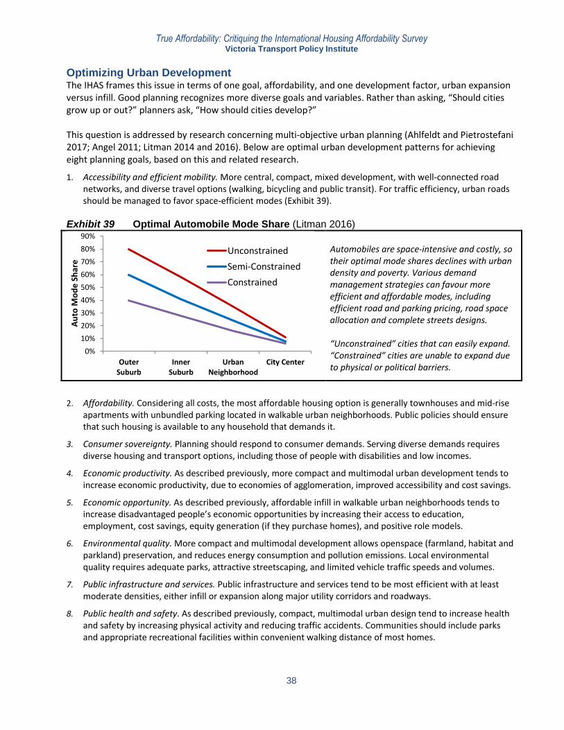
Optimizing Urban Development ........................................................................................................................ 38

Conclusions ........................................................................................................................................................ 40 Analysis Methods ............................................................................................................................................................40 IHAS Conclusions and Recommendations .......................................................................................................................41

References ......................................................................................................................................................... 42


3

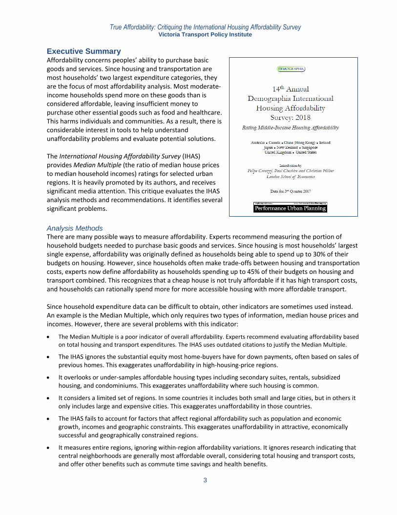
Executive Summary Affordability concerns peoples’ ability to purchase basic goods and services. Since housing and transportation are most households’ two largest expenditure categories, they are the focus of most affordability analysis. Most moderate-income households spend more on these goods than is considered affordable, leaving insufficient money to purchase other essential goods such as food and healthcare. This harms individuals and communities. As a result, there is considerable interest in tools to help understand unaffordability problems and evaluate potential solutions. The International Housing Affordability Survey (IHAS) provides Median Multiple (the ratio of median house prices to median household incomes) ratings for selected urban regions. It is heavily promoted by its authors, and receives significant media attention. This critique evaluates the IHAS analysis methods and recommendations. It identifies several significant problems.

Analysis Methods There are many possible ways to measure affordability. Experts recommend measuring the portion of household budgets needed to purchase basic goods and services. Since housing is most households’ largest single expense, affordability was originally defined as households being able to spend up to 30% of their budgets on housing. However, since households often make trade-offs between housing and transportation costs, experts now define affordability as households spending up to 45% of their budgets on housing and transport combined. This recognizes that a cheap house is not truly affordable if it has high transport costs, and households can rationally spend more for more accessible housing with more affordable transport. Since household expenditure data can be difficult to obtain, other indicators are sometimes used instead. An example is the Median Multiple, which only requires two types of information, median house prices and incomes. However, there are several problems with this indicator:

The Median Multiple is a poor indicator of overall affordability. Experts recommend evaluating affordability based on total housing and transport expenditures. The IHAS uses outdated citations to justify the Median Multiple.

The IHAS ignores the substantial equity most home-buyers have for down payments, often based on sales of previous homes. This exaggerates unaffordability in high-housing-price regions.

It overlooks or under-samples affordable housing types including secondary suites, rentals, subsidized housing, and condominiums. This exaggerates unaffordability where such housing is common.

It considers a limited set of regions. In some countries it includes both small and large cities, but in others it only includes large and expensive cities. This exaggerates unaffordability in those countries.

The IHAS fails to account for factors that affect regional affordability such as population and economic growth, incomes and geographic constraints. This exaggerates unaffordability in attractive, economically successful and geographically constrained regions.

It measures entire regions, ignoring within-region affordability variations. It ignores research indicating that central neighborhoods are generally most affordable overall, considering total housing and transport costs, and offer other benefits such as commute time savings and health benefits.


4

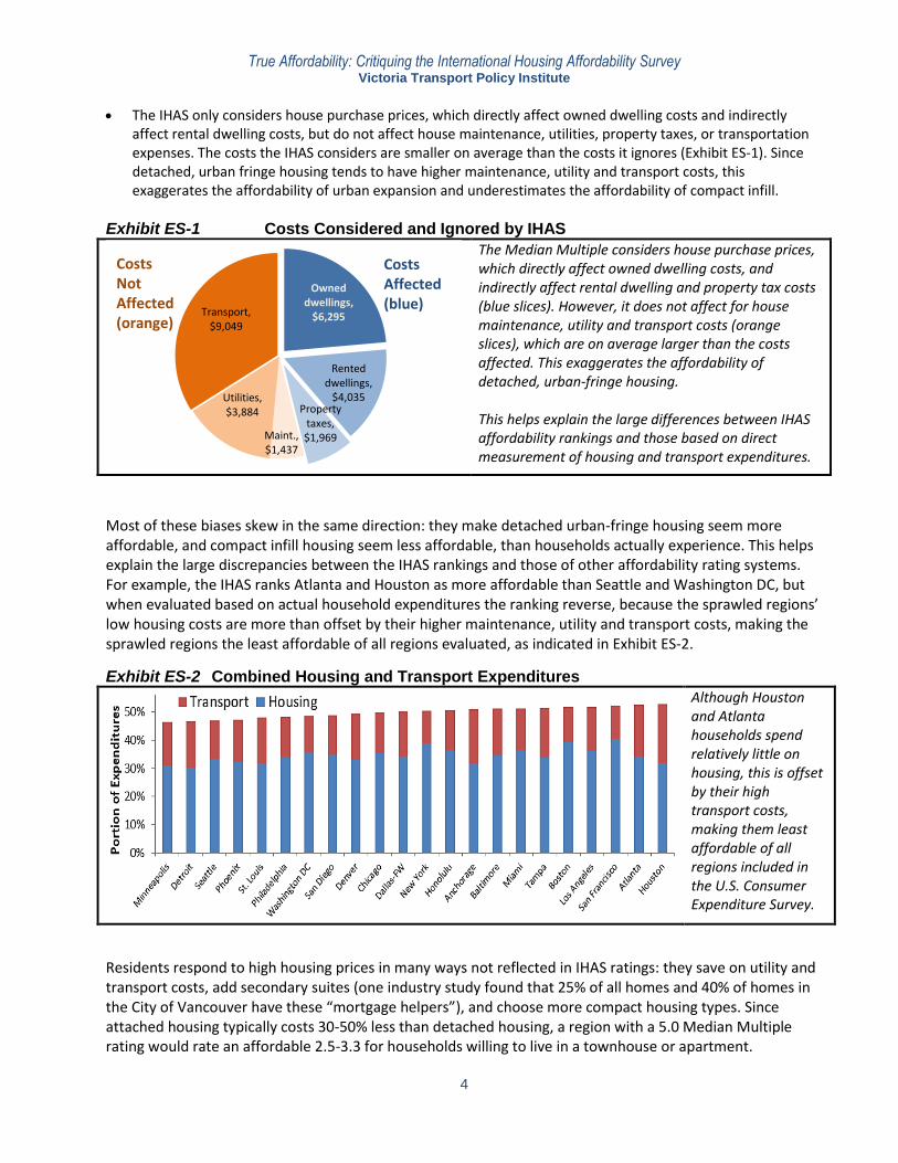
The IHAS only considers house purchase prices, which directly affect owned dwelling costs and indirectly affect rental dwelling costs, but do not affect house maintenance, utilities, property taxes, or transportation expenses. The costs the IHAS considers are smaller on average than the costs it ignores (Exhibit ES-1). Since detached, urban fringe housing tends to have higher maintenance, utility and transport costs, this exaggerates the affordability of urban expansion and underestimates the affordability of compact infill.

Exhibit ES-1 Costs Considered and Ignored by IHAS

The Median Multiple considers house purchase prices, which directly affect owned dwelling costs, and indirectly affect rental dwelling and property tax costs (blue slices). However, it does not affect for house maintenance, utility and transport costs (orange slices), which are on average larger than the costs affected. This exaggerates the affordability of detached, urban-fringe housing. This helps explain the large differences between IHAS affordability rankings and those based on direct measurement of housing and transport expenditures.

Most of these biases skew in the same direction: they make detached urban-fringe housing seem more affordable, and compact infill housing seem less affordable, than households actually experience. This helps explain the large discrepancies between the IHAS rankings and those of other affordability rating systems. For example, the IHAS ranks Atlanta and Houston as more affordable than Seattle and Washington DC, but when evaluated based on actual household expenditures the ranking reverse, because the sprawled regions’ low housing costs are more than offset by their higher maintenance, utility and transport costs, making the sprawled regions the least affordable of all regions evaluated, as indicated in Exhibit ES-2.

Exhibit ES-2 Combined Housing and Transport Expenditures

Although Houston and Atlanta households spend relatively little on housing, this is offset by their high transport costs, making them least affordable of all regions included in the U.S. Consumer Expenditure Survey.

Residents respond to high housing prices in many ways not reflected in IHAS ratings: they save on utility and transport costs, add secondary suites (one industry study found that 25% of all homes and 40% of homes in the City of Vancouver have these “mortgage helpers”), and choose more compact housing types. Since attached housing typically costs 30-50% less than detached housing, a region with a 5.0 Median Multiple rating would rate an affordable 2.5-3.3 for households willing to live in a townhouse or apartment.

Owned dwellings,

$6,295

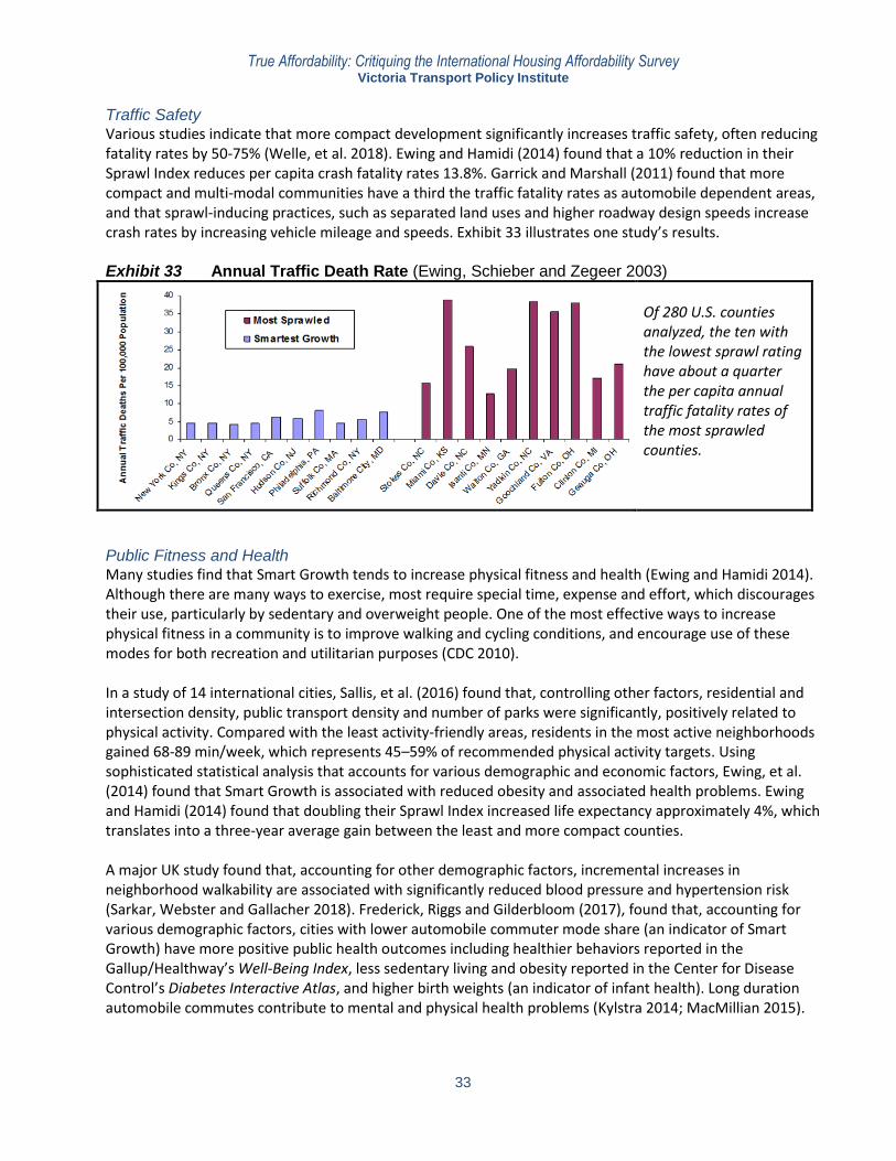
Rented dwellings,

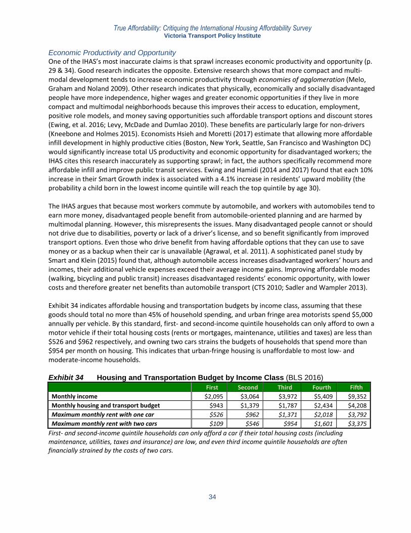
$4,035 Property

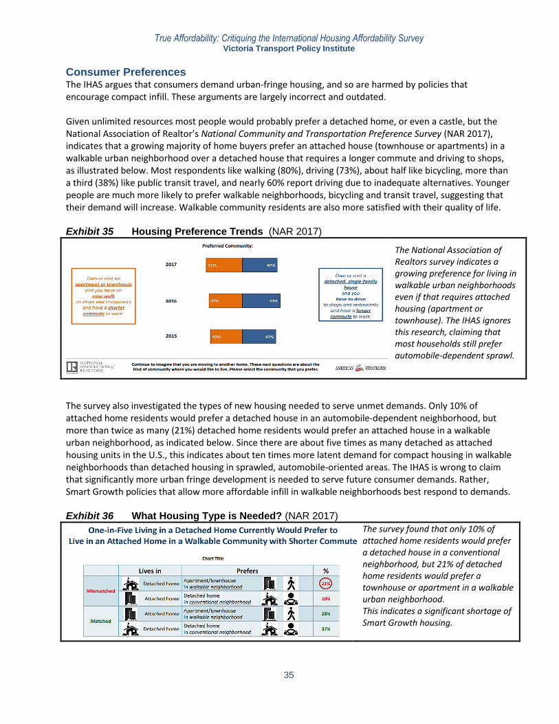
taxes, $1,969 Maint.,

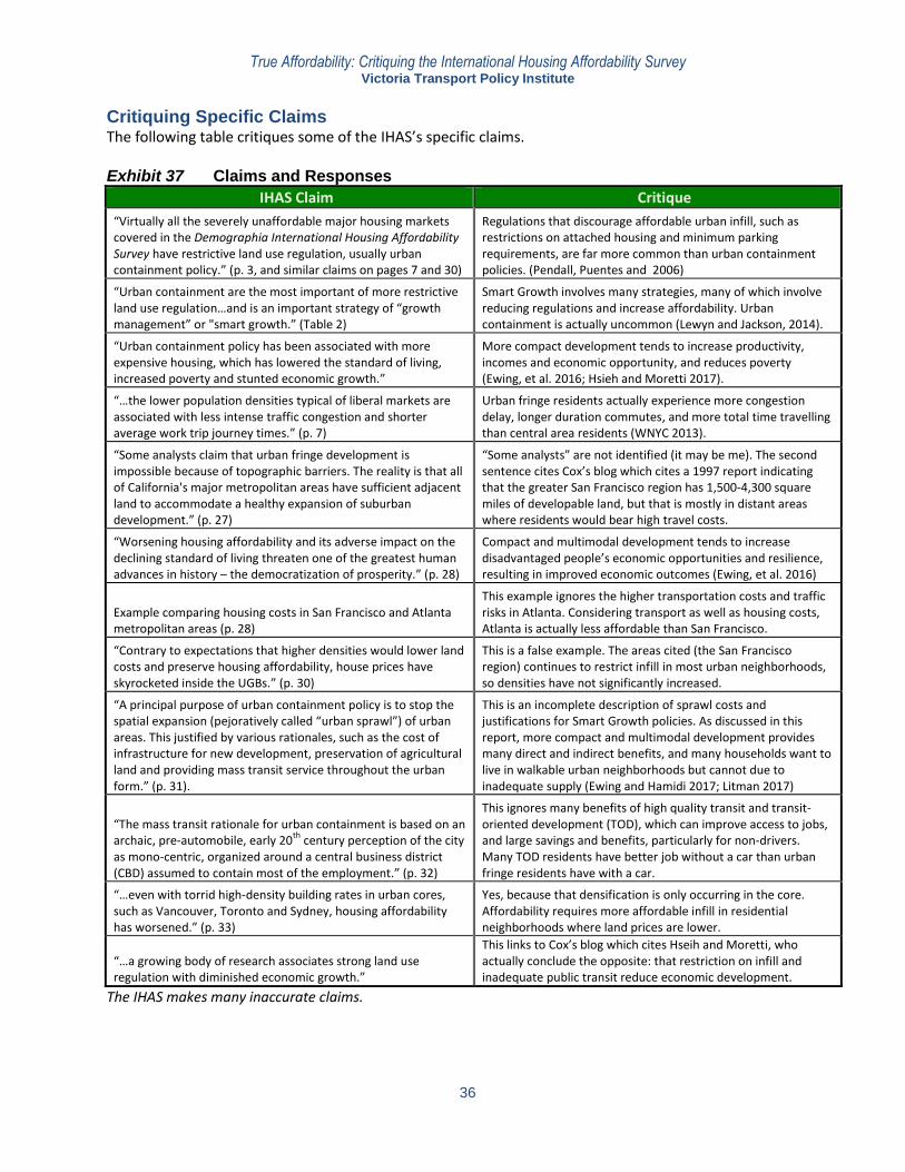
$1,437

Utilities, $3,884

Transport, $9,049

Costs Not Affected (orange)

Costs Affected (blue)


5

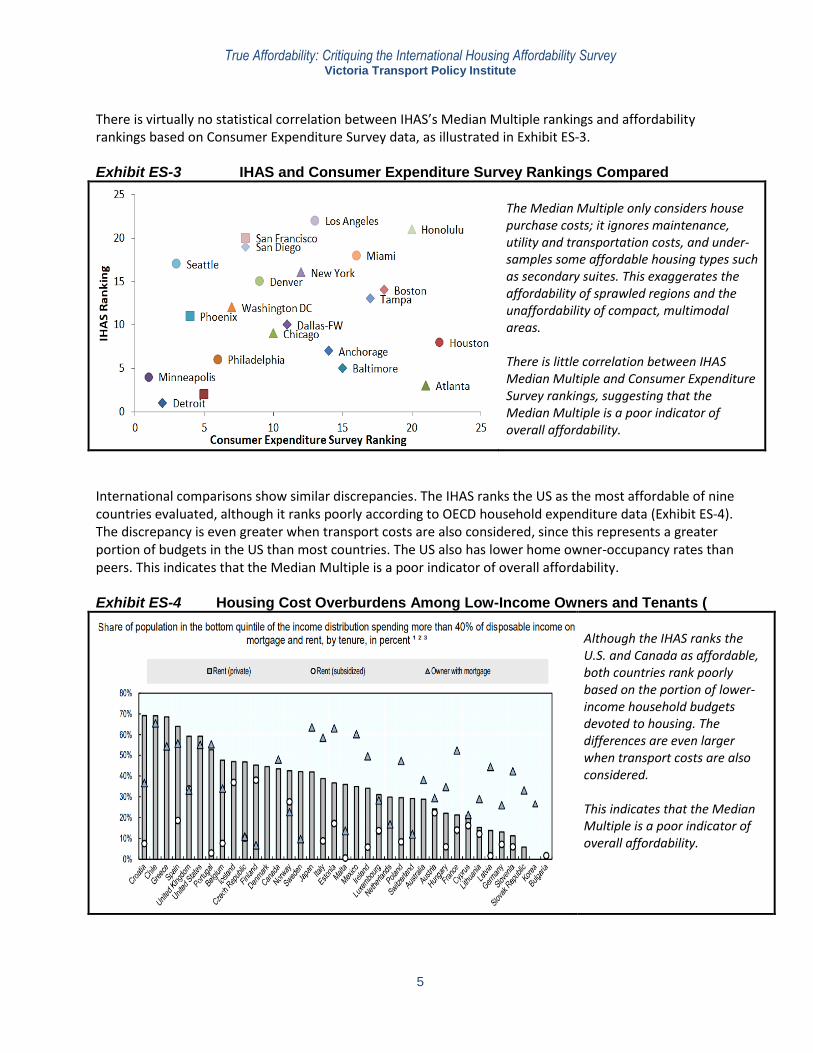
There is virtually no statistical correlation between IHAS’s Median Multiple rankings and affordability rankings based on Consumer Expenditure Survey data, as illustrated in Exhibit ES-3. Exhibit ES-3 IHAS and Consumer Expenditure Survey Rankings Compared

The Median Multiple only considers house purchase costs; it ignores maintenance, utility and transportation costs, and under-samples some affordable housing types such as secondary suites. This exaggerates the affordability of sprawled regions and the unaffordability of compact, multimodal areas. There is little correlation between IHAS Median Multiple and Consumer Expenditure Survey rankings, suggesting that the Median Multiple is a poor indicator of overall affordability.

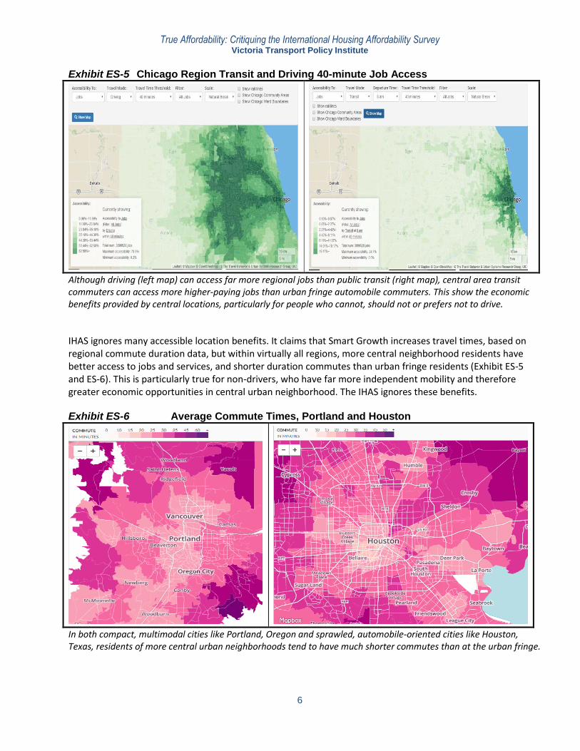
International comparisons show similar discrepancies. The IHAS ranks the US as the most affordable of nine countries evaluated, although it ranks poorly according to OECD household expenditure data (Exhibit ES-4). The discrepancy is even greater when transport costs are also considered, since this represents a greater portion of budgets in the US than most countries. The US also has lower home owner-occupancy rates than peers. This indicates that the Median Multiple is a poor indicator of overall affordability. Exhibit ES-4 Housing Cost Overburdens Among Low-Income Owners and Tenants (

Although the IHAS ranks the U.S. and Canada as affordable, both countries rank poorly based on the portion of lower-income household budgets devoted to housing. The differences are even larger when transport costs are also considered. This indicates that the Median Multiple is a poor indicator of overall affordability.


6

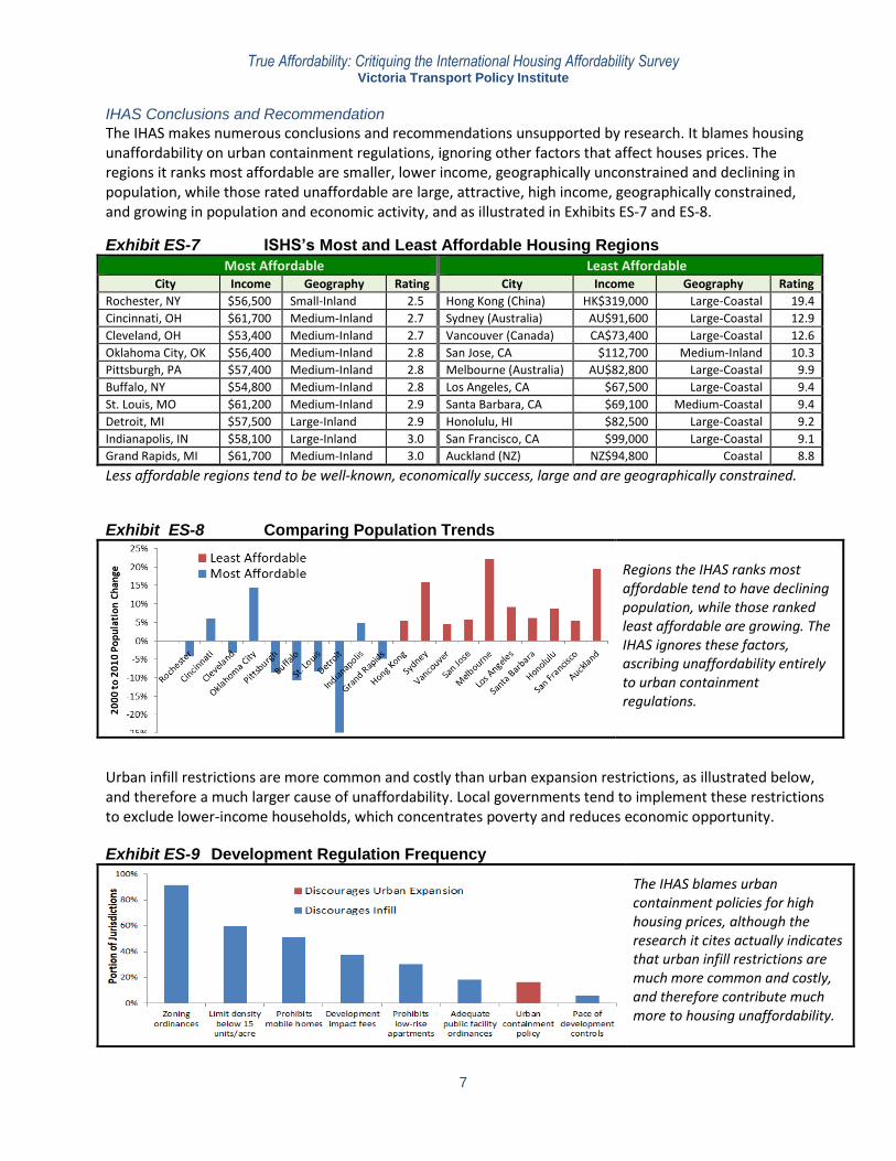
Exhibit ES-5 Chicago Region Transit and Driving 40-minute Job Access

Although driving (left map) can access far more regional jobs than public transit (right map), central area transit commuters can access more higher-paying jobs than urban fringe automobile commuters. This show the economic benefits provided by central locations, particularly for people who cannot, should not or prefers not to drive.

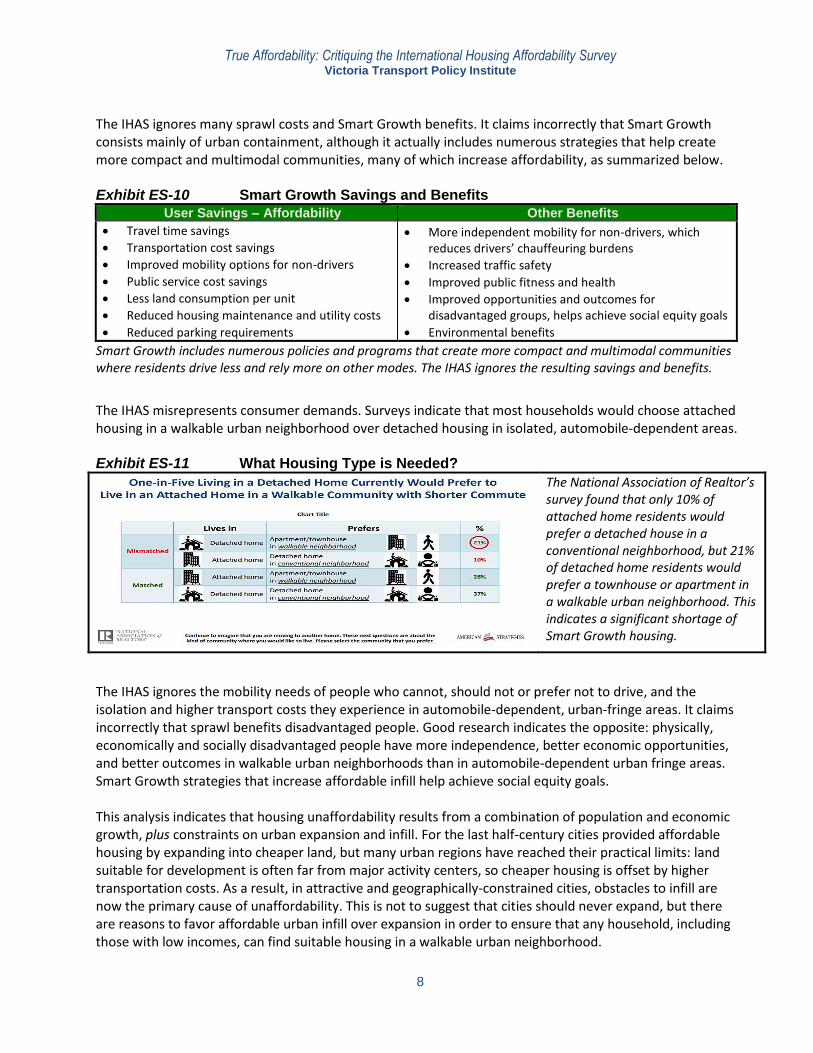
IHAS ignores many accessible location benefits. It claims that Smart Growth increases travel times, based on regional commute duration data, but within virtually all regions, more central neighborhood residents have better access to jobs and services, and shorter duration commutes than urban fringe residents (Exhibit ES-5 and ES-6). This is particularly true for non-drivers, who have far more independent mobility and therefore greater economic opportunities in central urban neighborhood. The IHAS ignores these benefits. Exhibit ES-6 Average Commute Times, Portland and Houston

In both compact, multimodal cities like Portland, Oregon and sprawled, automobile-oriented cities like Houston, Texas, residents of more central urban neighborhoods tend to have much shorter commutes than at the urban fringe.


7

IHAS Conclusions and Recommendation

The IHAS makes numerous conclusions and recommendations unsupported by research. It blames housing unaffordability on urban containment regulations, ignoring other factors that affect houses prices. The regions it ranks most affordable are smaller, lower income, geographically unconstrained and declining in population, while those rated unaffordable are large, attractive, high income, geographically constrained, and growing in population and economic activity, and as illustrated in Exhibits ES-7 and ES-8.

Exhibit ES-7 ISHS’s Most and Least Affordable Housing Regions

Most Affordable Least Affordable City Income Geography Rating City Income Geography Rating

Rochester, NY $56,500 Small-Inland 2.5 Hong Kong (China) HK$319,000 Large-Coastal 19.4

Cincinnati, OH $61,700 Medium-Inland 2.7 Sydney (Australia) AU$91,600 Large-Coastal 12.9

Cleveland, OH $53,400 Medium-Inland 2.7 Vancouver (Canada) CA$73,400 Large-Coastal 12.6

Oklahoma City, OK $56,400 Medium-Inland 2.8 San Jose, CA $112,700 Medium-Inland 10.3

Pittsburgh, PA $57,400 Medium-Inland 2.8 Melbourne (Australia) AU$82,800 Large-Coastal 9.9

Buffalo, NY $54,800 Medium-Inland 2.8 Los Angeles, CA $67,500 Large-Coastal 9.4

St. Louis, MO $61,200 Medium-Inland 2.9 Santa Barbara, CA $69,100 Medium-Coastal 9.4

Detroit, MI $57,500 Large-Inland 2.9 Honolulu, HI $82,500 Large-Coastal 9.2

Indianapolis, IN $58,100 Large-Inland 3.0 San Francisco, CA $99,000 Large-Coastal 9.1

Grand Rapids, MI $61,700 Medium-Inland 3.0 Auckland (NZ) NZ$94,800 Coastal 8.8

Less affordable regions tend to be well-known, economically success, large and are geographically constrained.

Exhibit ES-8 Comparing Population Trends

Regions the IHAS ranks most affordable tend to have declining population, while those ranked least affordable are growing. The IHAS ignores these factors, ascribing unaffordability entirely to urban containment regulations.

Urban infill restrictions are more common and costly than urban expansion restrictions, as illustrated below, and therefore a much larger cause of unaffordability. Local governments tend to implement these restrictions to exclude lower-income households, which concentrates poverty and reduces economic opportunity. Exhibit ES-9 Development Regulation Frequency

The IHAS blames urban containment policies for high housing prices, although the research it cites actually indicates that urban infill restrictions are much more common and costly, and therefore contribute much more to housing unaffordability.


8

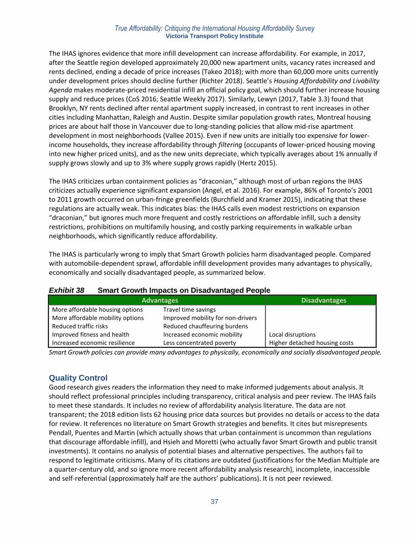
The IHAS ignores many sprawl costs and Smart Growth benefits. It claims incorrectly that Smart Growth consists mainly of urban containment, although it actually includes numerous strategies that help create more compact and multimodal communities, many of which increase affordability, as summarized below. Exhibit ES-10 Smart Growth Savings and Benefits

User Savings – Affordability Other Benefits

Travel time savings

Transportation cost savings

Improved mobility options for non-drivers

Public service cost savings

Less land consumption per unit

Reduced housing maintenance and utility costs

Reduced parking requirements

More independent mobility for non-drivers, which reduces drivers’ chauffeuring burdens

Increased traffic safety

Improved public fitness and health

Improved opportunities and outcomes for disadvantaged groups, helps achieve social equity goals

Environmental benefits

Smart Growth includes numerous policies and programs that create more compact and multimodal communities where residents drive less and rely more on other modes. The IHAS ignores the resulting savings and benefits.

The IHAS misrepresents consumer demands. Surveys indicate that most households would choose attached housing in a walkable urban neighborhood over detached housing in isolated, automobile-dependent areas. Exhibit ES-11 What Housing Type is Needed?

The National Association of Realtor’s survey found that only 10% of attached home residents would prefer a detached house in a conventional neighborhood, but 21% of detached home residents would prefer a townhouse or apartment in a walkable urban neighborhood. This indicates a significant shortage of Smart Growth housing.

The IHAS ignores the mobility needs of people who cannot, should not or prefer not to drive, and the isolation and higher transport costs they experience in automobile-dependent, urban-fringe areas. It claims incorrectly that sprawl benefits disadvantaged people. Good research indicates the opposite: physically, economically and socially disadvantaged people have more independence, better economic opportunities, and better outcomes in walkable urban neighborhoods than in automobile-dependent urban fringe areas. Smart Growth strategies that increase affordable infill help achieve social equity goals. This analysis indicates that housing unaffordability results from a combination of population and economic growth, plus constraints on urban expansion and infill. For the last half-century cities provided affordable housing by expanding into cheaper land, but many urban regions have reached their practical limits: land suitable for development is often far from major activity centers, so cheaper housing is offset by higher transportation costs. As a result, in attractive and geographically-constrained cities, obstacles to infill are now the primary cause of unaffordability. This is not to suggest that cities should never expand, but there are reasons to favor affordable urban infill over expansion in order to ensure that any household, including those with low incomes, can find suitable housing in a walkable urban neighborhood.


9

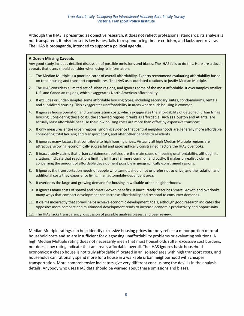
Although the IHAS is presented as objective research, it does not reflect professional standards: its analysis is not transparent, it misrepresents key issues, fails to respond to legitimate criticism, and lacks peer review. The IHAS is propaganda, intended to support a political agenda.

A Dozen Missing Caveats Any good study includes detailed discussion of possible omissions and biases. The IHAS fails to do this. Here are a dozen caveats that users should consider when using its information.

1. The Median Multiple is a poor indicator of overall affordability. Experts recommend evaluating affordability based on total housing and transport expenditures. The IHAS uses outdated citations to justify Median Multiple.

2. The IHAS considers a limited set of urban regions, and ignores some of the most affordable. It oversamples smaller U.S. and Canadian regions, which exaggerates North American affordability.

3. It excludes or under-samples some affordable housing types, including secondary suites, condominiums, rentals and subsidized housing. This exaggerates unaffordability in areas where such housing is common.

4. It ignores house operation and transportation costs, which exaggerates the affordability of detached, urban fringe housing. Considering these costs, the sprawled regions it ranks as affordable, such as Houston and Atlanta, are actually least affordable because their low housing costs are more than offset by expensive transport.

5. It only measures entire urban regions, ignoring evidence that central neighborhoods are generally more affordable, considering total housing and transport costs, and offer other benefits to residents.

6. It ignores many factors that contribute to high housing prices. Virtually all high Median Multiple regions are attractive, growing, economically successful and geographically constrained, factors the IHAS overlooks.

7. It inaccurately claims that urban containment policies are the main cause of housing unaffordability, although its citations indicate that regulations limiting infill are far more common and costly. It makes unrealistic claims concerning the amount of affordable development possible in geographically-constrained regions.

8. It ignores the transportation needs of people who cannot, should not or prefer not to drive, and the isolation and additional costs they experience living in an automobile-dependent area.

9. It overlooks the large and growing demand for housing in walkable urban neighborhoods.

10. It ignores many costs of sprawl and Smart Growth benefits. It inaccurately describes Smart Growth and overlooks many ways that compact development can increase affordability and respond to consumer demands.

11. It claims incorrectly that sprawl helps achieve economic development goals, although good research indicates the opposite: more compact and multimodal development tends to increase economic productivity and opportunity.

12. The IHAS lacks transparency, discussion of possible analysis biases, and peer review.

Median Multiple ratings can help identify excessive housing prices but only reflect a minor portion of total household costs and so are insufficient for diagnosing unaffordability problems or evaluating solutions. A high Median Multiple rating does not necessarily mean that most households suffer excessive cost burdens, nor does a low rating indicate that an area is affordable overall. The IHAS ignores basic household economics: a cheap house is not truly affordable if located in an isolated area with high transport costs, and households can rationally spend more for a house in a walkable urban neighborhood with cheaper transportation. More comprehensive indicators give very different conclusions; the devil is in the analysis details. Anybody who uses IHAS data should be warned about these omissions and biases.


10

Introduction

You can't always get what you want (3x) But if you try sometimes you might find You get what you need - Keith Richards & Sir Mick Jagger (1969), The Rolling Stones

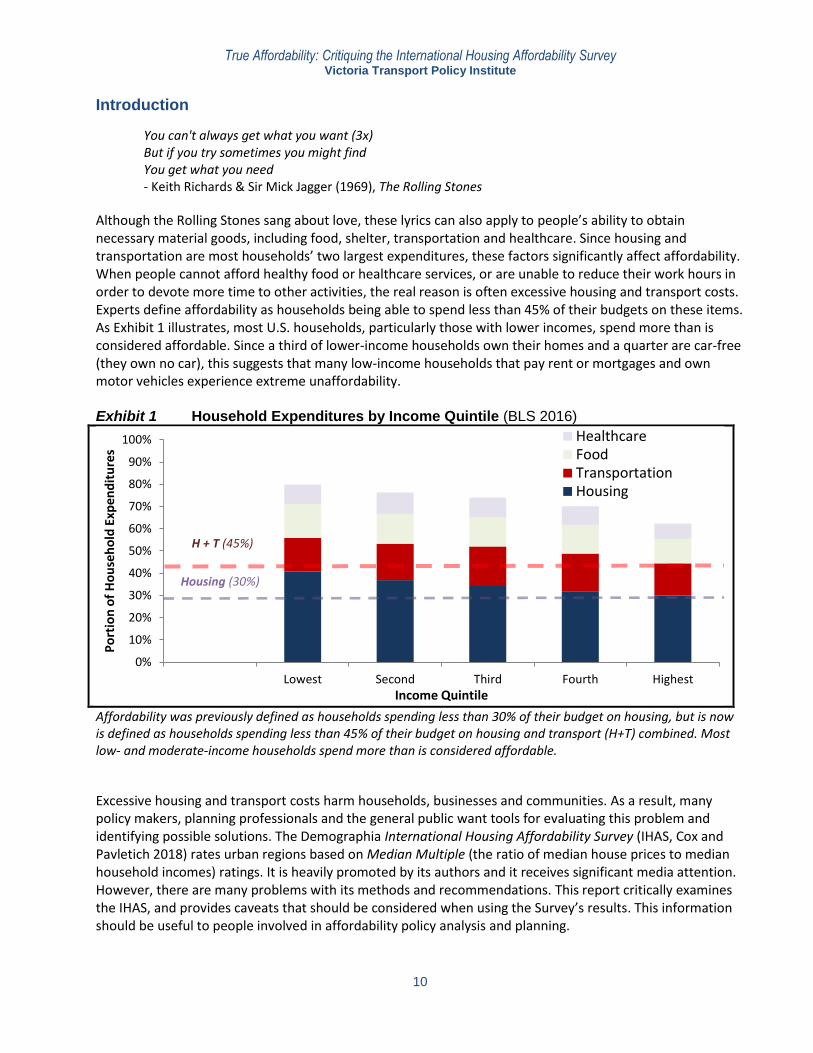
Although the Rolling Stones sang about love, these lyrics can also apply to people’s ability to obtain necessary material goods, including food, shelter, transportation and healthcare. Since housing and transportation are most households’ two largest expenditures, these factors significantly affect affordability. When people cannot afford healthy food or healthcare services, or are unable to reduce their work hours in order to devote more time to other activities, the real reason is often excessive housing and transport costs. Experts define affordability as households being able to spend less than 45% of their budgets on these items. As Exhibit 1 illustrates, most U.S. households, particularly those with lower incomes, spend more than is considered affordable. Since a third of lower-income households own their homes and a quarter are car-free (they own no car), this suggests that many low-income households that pay rent or mortgages and own motor vehicles experience extreme unaffordability. Exhibit 1 Household Expenditures by Income Quintile (BLS 2016)

Affordability was previously defined as households spending less than 30% of their budget on housing, but is now is defined as households spending less than 45% of their budget on housing and transport (H+T) combined. Most low- and moderate-income households spend more than is considered affordable.

Excessive housing and transport costs harm households, businesses and communities. As a result, many policy makers, planning professionals and the general public want tools for evaluating this problem and identifying possible solutions. The Demographia International Housing Affordability Survey (IHAS, Cox and Pavletich 2018) rates urban regions based on Median Multiple (the ratio of median house prices to median household incomes) ratings. It is heavily promoted by its authors and it receives significant media attention. However, there are many problems with its methods and recommendations. This report critically examines the IHAS, and provides caveats that should be considered when using the Survey’s results. This information should be useful to people involved in affordability policy analysis and planning.

0%

10%

20%

30%

40%

50%

60%

70%

80%

90%

100%

Lowest Second Third Fourth Highest

Po

rtio

n o

f H

ou

seh

old

Exp

end

itu

res

Income Quintile

HealthcareFoodTransportationHousing

Housing (30%)

H + T (45%)


11

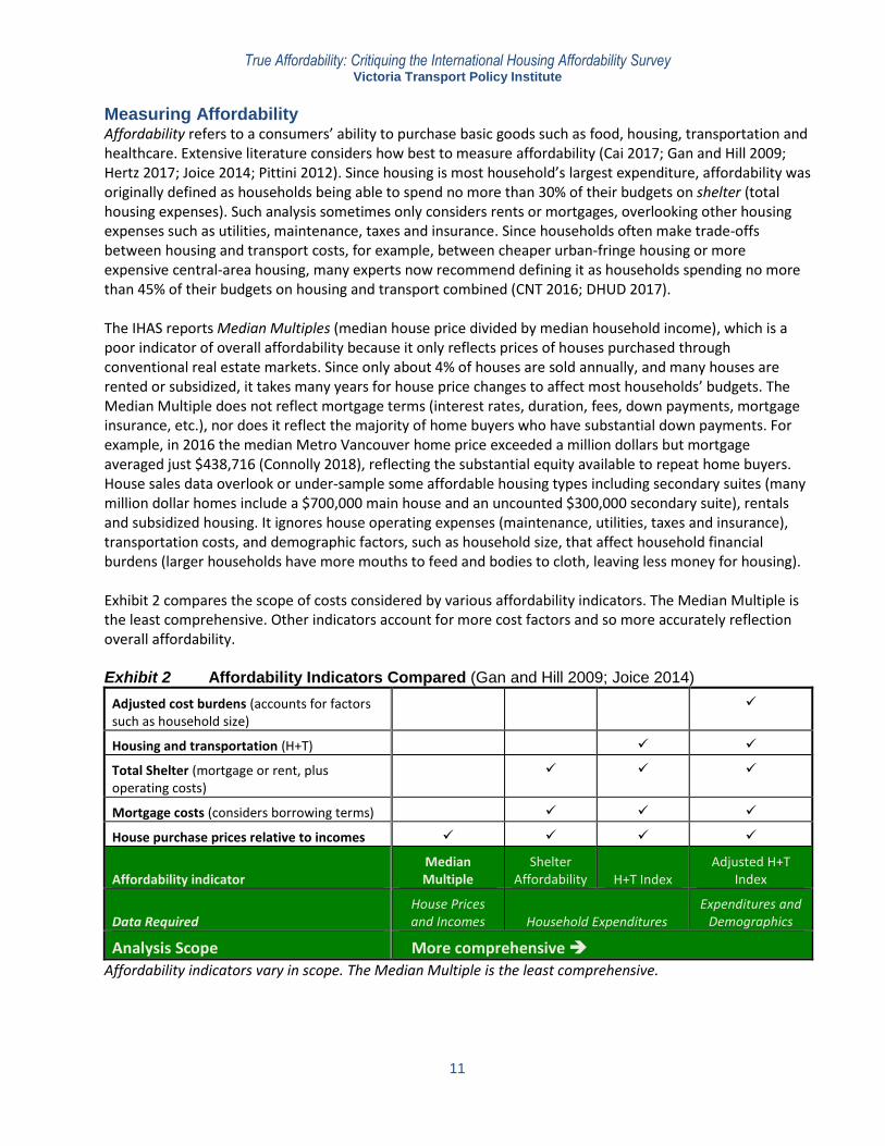
Measuring Affordability Affordability refers to a consumers’ ability to purchase basic goods such as food, housing, transportation and healthcare. Extensive literature considers how best to measure affordability (Cai 2017; Gan and Hill 2009; Hertz 2017; Joice 2014; Pittini 2012). Since housing is most household’s largest expenditure, affordability was originally defined as households being able to spend no more than 30% of their budgets on shelter (total housing expenses). Such analysis sometimes only considers rents or mortgages, overlooking other housing expenses such as utilities, maintenance, taxes and insurance. Since households often make trade-offs between housing and transport costs, for example, between cheaper urban-fringe housing or more expensive central-area housing, many experts now recommend defining it as households spending no more than 45% of their budgets on housing and transport combined (CNT 2016; DHUD 2017). The IHAS reports Median Multiples (median house price divided by median household income), which is a poor indicator of overall affordability because it only reflects prices of houses purchased through conventional real estate markets. Since only about 4% of houses are sold annually, and many houses are rented or subsidized, it takes many years for house price changes to affect most households’ budgets. The Median Multiple does not reflect mortgage terms (interest rates, duration, fees, down payments, mortgage insurance, etc.), nor does it reflect the majority of home buyers who have substantial down payments. For example, in 2016 the median Metro Vancouver home price exceeded a million dollars but mortgage averaged just $438,716 (Connolly 2018), reflecting the substantial equity available to repeat home buyers. House sales data overlook or under-sample some affordable housing types including secondary suites (many million dollar homes include a $700,000 main house and an uncounted $300,000 secondary suite), rentals and subsidized housing. It ignores house operating expenses (maintenance, utilities, taxes and insurance), transportation costs, and demographic factors, such as household size, that affect household financial burdens (larger households have more mouths to feed and bodies to cloth, leaving less money for housing). Exhibit 2 compares the scope of costs considered by various affordability indicators. The Median Multiple is the least comprehensive. Other indicators account for more cost factors and so more accurately reflection overall affordability. Exhibit 2 Affordability Indicators Compared (Gan and Hill 2009; Joice 2014)

Adjusted cost burdens (accounts for factors such as household size)

Housing and transportation (H+T)

Total Shelter (mortgage or rent, plus operating costs)

Mortgage costs (considers borrowing terms)

House purchase prices relative to incomes

Affordability indicator Median Multiple

Shelter Affordability H+T Index

Adjusted H+T Index

Data Required House Prices and Incomes Household Expenditures

Expenditures and Demographics

Analysis Scope More comprehensive

Affordability indicators vary in scope. The Median Multiple is the least comprehensive.


12

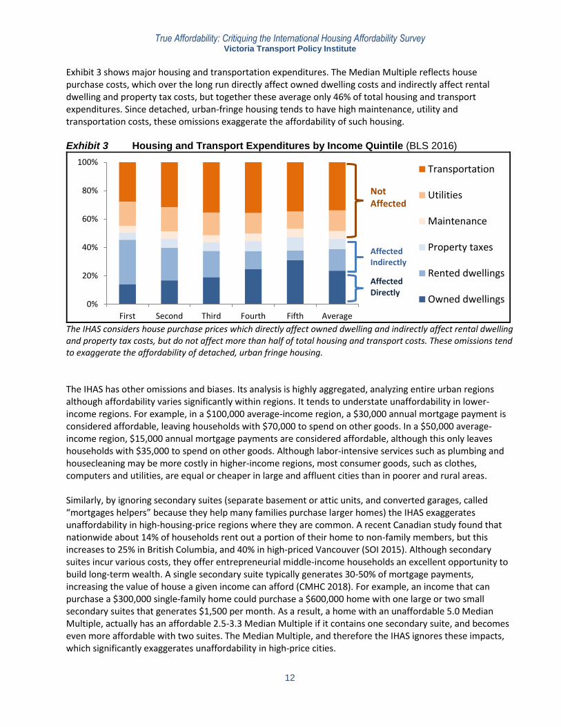
Exhibit 3 shows major housing and transportation expenditures. The Median Multiple reflects house purchase costs, which over the long run directly affect owned dwelling costs and indirectly affect rental dwelling and property tax costs, but together these average only 46% of total housing and transport expenditures. Since detached, urban-fringe housing tends to have high maintenance, utility and transportation costs, these omissions exaggerate the affordability of such housing. Exhibit 3 Housing and Transport Expenditures by Income Quintile (BLS 2016)

The IHAS considers house purchase prices which directly affect owned dwelling and indirectly affect rental dwelling and property tax costs, but do not affect more than half of total housing and transport costs. These omissions tend to exaggerate the affordability of detached, urban fringe housing.

The IHAS has other omissions and biases. Its analysis is highly aggregated, analyzing entire urban regions although affordability varies significantly within regions. It tends to understate unaffordability in lower-income regions. For example, in a $100,000 average-income region, a $30,000 annual mortgage payment is considered affordable, leaving households with $70,000 to spend on other goods. In a $50,000 average-income region, $15,000 annual mortgage payments are considered affordable, although this only leaves households with $35,000 to spend on other goods. Although labor-intensive services such as plumbing and housecleaning may be more costly in higher-income regions, most consumer goods, such as clothes, computers and utilities, are equal or cheaper in large and affluent cities than in poorer and rural areas. Similarly, by ignoring secondary suites (separate basement or attic units, and converted garages, called “mortgages helpers” because they help many families purchase larger homes) the IHAS exaggerates unaffordability in high-housing-price regions where they are common. A recent Canadian study found that nationwide about 14% of households rent out a portion of their home to non-family members, but this increases to 25% in British Columbia, and 40% in high-priced Vancouver (SOI 2015). Although secondary suites incur various costs, they offer entrepreneurial middle-income households an excellent opportunity to build long-term wealth. A single secondary suite typically generates 30-50% of mortgage payments, increasing the value of house a given income can afford (CMHC 2018). For example, an income that can purchase a $300,000 single-family home could purchase a $600,000 home with one large or two small secondary suites that generates $1,500 per month. As a result, a home with an unaffordable 5.0 Median Multiple, actually has an affordable 2.5-3.3 Median Multiple if it contains one secondary suite, and becomes even more affordable with two suites. The Median Multiple, and therefore the IHAS ignores these impacts, which significantly exaggerates unaffordability in high-price cities.

0%

20%

40%

60%

80%

100%

First Second Third Fourth Fifth Average

Transportation

Utilities

Maintenance

Property taxes

Rented dwellings

Owned dwellings

Affected Directly

Not Affected

Affected Indirectly


13

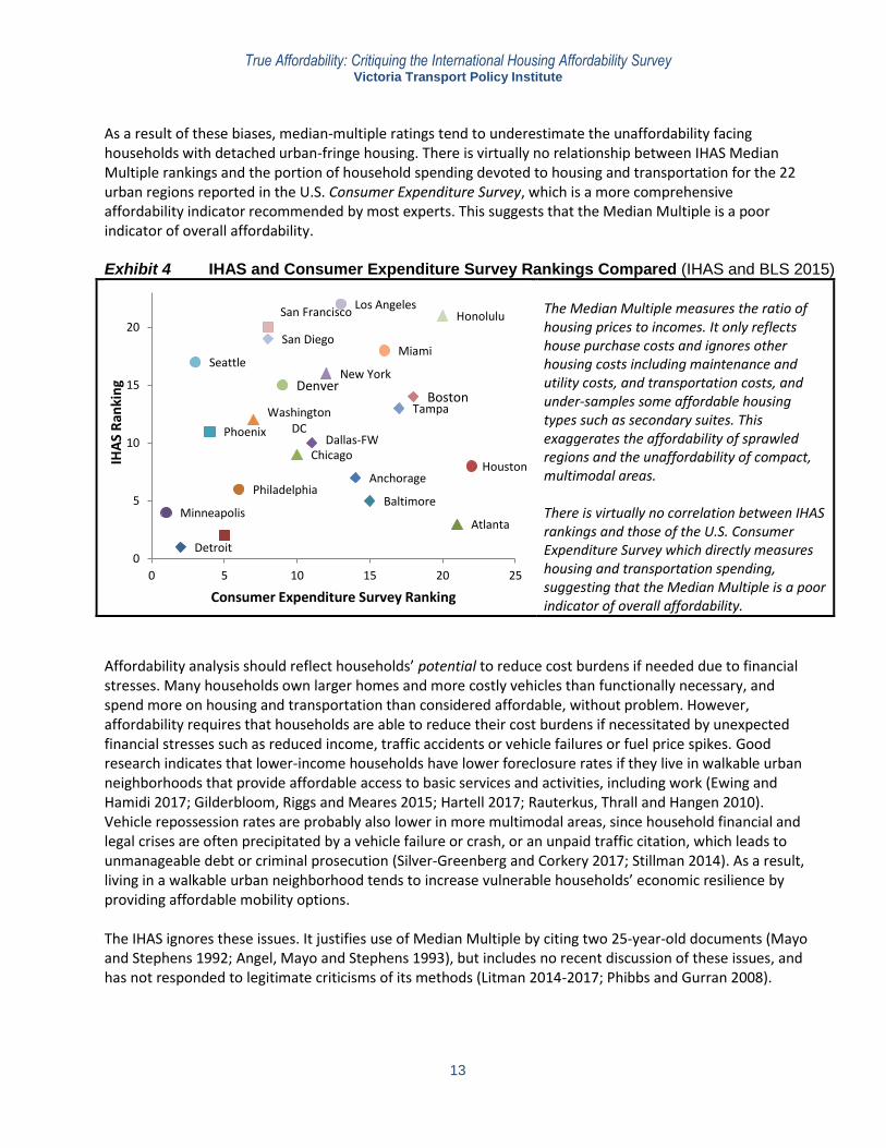
As a result of these biases, median-multiple ratings tend to underestimate the unaffordability facing households with detached urban-fringe housing. There is virtually no relationship between IHAS Median Multiple rankings and the portion of household spending devoted to housing and transportation for the 22 urban regions reported in the U.S. Consumer Expenditure Survey, which is a more comprehensive affordability indicator recommended by most experts. This suggests that the Median Multiple is a poor indicator of overall affordability. Exhibit 4 IHAS and Consumer Expenditure Survey Rankings Compared (IHAS and BLS 2015)

The Median Multiple measures the ratio of housing prices to incomes. It only reflects house purchase costs and ignores other housing costs including maintenance and utility costs, and transportation costs, and under-samples some affordable housing types such as secondary suites. This exaggerates the affordability of sprawled regions and the unaffordability of compact, multimodal areas. There is virtually no correlation between IHAS rankings and those of the U.S. Consumer Expenditure Survey which directly measures housing and transportation spending, suggesting that the Median Multiple is a poor indicator of overall affordability.

Affordability analysis should reflect households’ potential to reduce cost burdens if needed due to financial stresses. Many households own larger homes and more costly vehicles than functionally necessary, and spend more on housing and transportation than considered affordable, without problem. However, affordability requires that households are able to reduce their cost burdens if necessitated by unexpected financial stresses such as reduced income, traffic accidents or vehicle failures or fuel price spikes. Good research indicates that lower-income households have lower foreclosure rates if they live in walkable urban neighborhoods that provide affordable access to basic services and activities, including work (Ewing and Hamidi 2017; Gilderbloom, Riggs and Meares 2015; Hartell 2017; Rauterkus, Thrall and Hangen 2010). Vehicle repossession rates are probably also lower in more multimodal areas, since household financial and legal crises are often precipitated by a vehicle failure or crash, or an unpaid traffic citation, which leads to unmanageable debt or criminal prosecution (Silver-Greenberg and Corkery 2017; Stillman 2014). As a result, living in a walkable urban neighborhood tends to increase vulnerable households’ economic resilience by providing affordable mobility options. The IHAS ignores these issues. It justifies use of Median Multiple by citing two 25-year-old documents (Mayo and Stephens 1992; Angel, Mayo and Stephens 1993), but includes no recent discussion of these issues, and has not responded to legitimate criticisms of its methods (Litman 2014-2017; Phibbs and Gurran 2008).

Detroit

Atlanta Minneapolis

Baltimore Philadelphia

Anchorage Houston

Chicago Dallas-FW

Phoenix

Washington DC

Tampa Boston

Denver New York

Seattle Miami

San Diego

San Francisco Honolulu Los Angeles

0

5

10

15

20

0 5 10 15 20 25

IHA

S R

anki

ng

Consumer Expenditure Survey Ranking


14

What Housing is Most Affordable? The IHAS reflects “top down” analysis that measures aggregate impacts. It is useful to also apply “bottom up” analysis that examines individual factors that affect affordability. This considers the following factors.

1. Public Infrastructure and Services Public infrastructure and services include roads, utility lines, emergency services and school transportation. They tend to be lower for compact infill than urban fringe development (Litman 2017; Ewing and Hamidi 2017). For example, Smart Growth & Conventional Suburban Development: Which Costs More? (Ford 2010) found that compact development typically reduces infrastructure costs 30-50%, and Building Better Budgets (SGA 2013), found it reduces infrastructure costs by a third and ongoing public service costs 10%.

2. Land Although land prices tend to be higher in urban neighborhoods than at the urban fringe, this can be offset by increased density which reduces land consumption per housing unit. Detached housing (2-10 unit per acre) typically requires ten times as much land per unit as townhouses (20-40 units per acre), twenty times as much as mid-rise (40-80 units per acre), and forty times as much as high-rise housing (100+ units per acre).

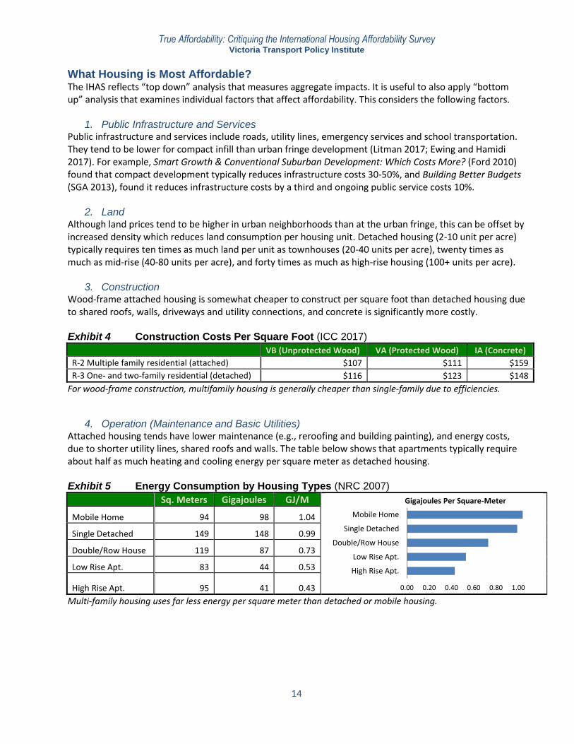
3. Construction Wood-frame attached housing is somewhat cheaper to construct per square foot than detached housing due to shared roofs, walls, driveways and utility connections, and concrete is significantly more costly. Exhibit 4 Construction Costs Per Square Foot (ICC 2017)

VB (Unprotected Wood) VA (Protected Wood) IA (Concrete)

R-2 Multiple family residential (attached) $107 $111 $159

R-3 One- and two-family residential (detached) $116 $123 $148

For wood-frame construction, multifamily housing is generally cheaper than single-family due to efficiencies.

4. Operation (Maintenance and Basic Utilities) Attached housing tends have lower maintenance (e.g., reroofing and building painting), and energy costs, due to shorter utility lines, shared roofs and walls. The table below shows that apartments typically require about half as much heating and cooling energy per square meter as detached housing. Exhibit 5 Energy Consumption by Housing Types (NRC 2007)

Sq. Meters Gigajoules GJ/M

Mobile Home 94 98 1.04

Single Detached 149 148 0.99

Double/Row House 119 87 0.73

Low Rise Apt. 83 44 0.53

High Rise Apt. 95 41 0.43

Multi-family housing uses far less energy per square meter than detached or mobile housing.

0.00 0.20 0.40 0.60 0.80 1.00

High Rise Apt.

Low Rise Apt.

Double/Row House

Single Detached

Mobile Home

Gigajoules Per Square-Meter


15

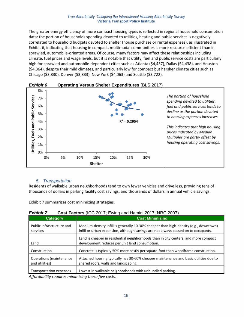
The greater energy efficiency of more compact housing types is reflected in regional household consumption data: the portion of households spending devoted to utilities, heating and public services is negatively correlated to household budgets devoted to shelter (house purchase or rental expenses), as illustrated in Exhibit 6, indicating that housing in compact, multimodal communities is more resource efficient than in sprawled, automobile-oriented areas. Of course, many factors may affect these relationships including climate, fuel prices and wage levels, but it is notable that utility, fuel and public service costs are particularly high for sprawled and automobile-dependent cities such as Atlanta ($4,437), Dallas ($4,438), and Houston ($4,364), despite their mild climates, and particularly low for compact but harsher climate cities such as Chicago ($3,830), Denver ($3,833), New York ($4,063) and Seattle ($3,722). Exhibit 6 Operating Versus Shelter Expenditures (BLS 2017)

The portion of household spending devoted to utilities, fuel and public services tends to decline as the portion devoted to housing expenses increases. This indicates that high housing prices indicated by Median Multiples are partly offset by housing operating cost savings.

5. Transportation Residents of walkable urban neighborhoods tend to own fewer vehicles and drive less, providing tens of thousands of dollars in parking facility cost savings, and thousands of dollars in annual vehicle savings. Exhibit 7 summarizes cost minimizing strategies.

Exhibit 7 Cost Factors (ICC 2017; Ewing and Hamidi 2017; NRC 2007)

Category Cost Minimizing

Public infrastructure and services

Medium-density Infill is generally 10-30% cheaper than high-density (e.g., downtown) infill or urban expansion, although savings are not always passed on to occupants.

Land Land is cheaper in residential neighborhoods than in city centers, and more compact development reduces per unit land consumption.

Construction Concrete is typically 50% more costly per square-foot than woodframe construction.

Operations (maintenance and utilities)

Attached housing typically has 30-60% cheaper maintenance and basic utilities due to shared roofs, walls and landscaping.

Transportation expenses Lowest in walkable neighborhoods with unbundled parking.

Affordability requires minimizing these five costs.

R² = 0.2954

0%

1%

2%

3%

4%

5%

6%

7%

8%

0% 5% 10% 15% 20% 25% 30%

Uti

litie

s, F

uel

s an

d P

ub

lic S

erv

ice

s

Shelter


16

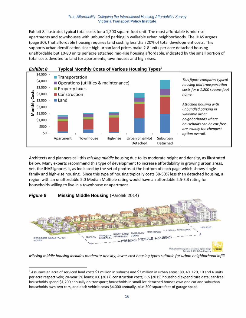
Exhibit 8 illustrates typical total costs for a 1,200 square-foot unit. The most affordable is mid-rise apartments and townhouses with unbundled parking in walkable urban neighborhoods. The IHAS argues (page 30), that affordable housing requires land costing less than 20% of total development costs. This supports urban densification since high urban land prices make 2-8 units per acre detached housing unaffordable but 10-80 units per acre attached mid-rise housing affordable, indicated by the small portion of total costs devoted to land for apartments, townhouses and high rises. Exhibit 8 Typical Monthly Costs of Various Housing Types1

This figure compares typical housing and transportation costs for a 1,200 square-foot home. Attached housing with unbundled parking in walkable urban neighborhoods where households can be car-free are usually the cheapest option overall.

Architects and planners call this missing middle housing due to its moderate height and density, as illustrated below. Many experts recommend this type of development to increase affordability in growing urban areas, yet, the IHAS ignores it, as indicated by the set of photos at the bottom of each page which shows single-family and high-rise housing. Since this type of housing typically costs 30-50% less than detached housing, a region with an unaffordable 5.0 Median Multiple rating would have an affordable 2.5-3.3 rating for households willing to live in a townhouse or apartment. Figure 9 Missing Middle Housing (Parolek 2014)

Missing middle housing includes moderate-density, lower-cost housing types suitable for urban neighborhood infill.

1 Assumes an acre of serviced land costs $1 million in suburbs and $2 million in urban areas; 80, 40, 120, 10 and 4 units

per acre respectively; 20-year 5% loans; ICC (2017) construction costs; BLS (2015) household expenditure data; car-free households spend $1,200 annually on transport; households in small-lot detached houses own one car and suburban households own two cars, and each vehicle costs $4,000 annually, plus 300 square feet of garage space.

$0

$500

$1,000

$1,500

$2,000

$2,500

$3,000

$3,500

$4,000

$4,500

Apartment Townhouse High-rise Urban Small-lotDetached

SuburbanDetached

Mo

nth

ly C

ost

s

TransportationOperations (utilities & maintenance)Property taxesConstructionLand


17

Despite its low construction and operating costs, missing middle infill is often more costly to develop than detached, urban-fringe housing due to regulations which prohibit multifamily housing in residential neighborhoods, unjustified parking requirements, and other restrictions and fees that add costs and delays. These regulations and fees add relatively little to the overall costs of expensive housing, but significantly increase lower-priced housing costs. By discouraging affordable infill development these policies tend to concentrate poverty and associated social problems, and create the need for subsidized housing (Hirt 2014). This explains why countries with national housing policies that limit local government regulations, such as Germany and Japan, tend to have more affordable housing (Fingleton 2014; Harding 2016). Cecchini (2015), Lewyn (2017) and the Sightline Institute (2016) analyze factors that discourage affordable infill development and identify policy reforms to make it more feasible, such as allowing compact housing types in residential neighborhoods, reduced and more flexible parking requirements, and improving affordable local travel options, but IHAS opposes these Smart Growth strategies. Other factors can drive up housing prices in attractive and economically successful cities, including tourist accommodations and businesses that compete for available housing stock, foreign investments, and real estate speculation. However, these impacts are often exaggerated. For example, only 3.4% of Vancouver homes and 4.8% of Toronto homes are foreign owned, which is insufficient to explain their high housing prices (Mahoney 2017). These factors only contribute to price escalation if housing supply is limited and unresponsive to growing demand (Durning 2017).


18

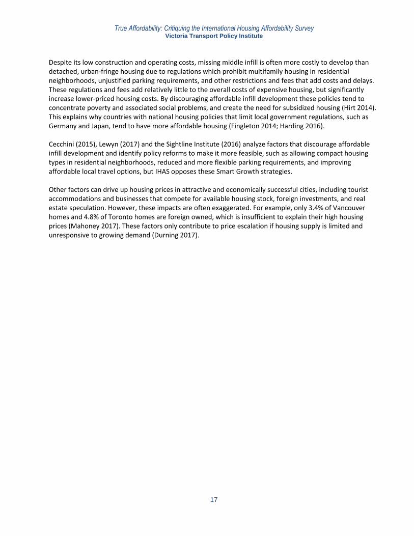
Geographic Scope The IHAS includes data from nine countries (Australia, Canada, China [Hong Kong], Ireland, Japan, New Zealand, Singapore, the UK and the US), which excludes many affordable markets. For example, North Americans spend a larger portion of budgets on housing than in most peer countries (Exhibit 10). Exhibit 10 Housing Cost Burden as a Share of Disposable Income (OECD 2017)

The US and Canada rank 14th and 15th out of 38 OECD countries in rent and mortgage cost burdens.

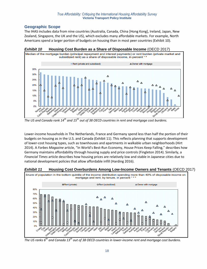
Lower-income households in The Netherlands, France and Germany spend less than half the portion of their budgets on housing as in the U.S. and Canada (Exhibit 11). This reflects planning that supports development of lower-cost housing types, such as townhouses and apartments in walkable urban neighborhoods (Hirt 2014). A Forbes Magazine article, “In World’s Best-Run Economy, House Prices Keep Falling,” describes how Germany maintains affordability through housing supply and price controls (Fingleton 2014). Similarly, a Financial Times article describes how housing prices are relatively low and stable in Japanese cities due to national development policies that allow affordable infill (Harding 2016).

Exhibit 11 Housing Cost Overburdens Among Low-Income Owners and Tenants (OECD 2017)

The US ranks 6th and Canada 13th out of 38 OECD countries in lower-income rent and mortgage cost burdens.


19

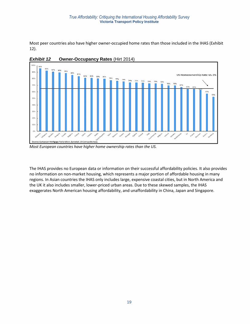
Most peer countries also have higher owner-occupied home rates than those included in the IHAS (Exhibit 12). Exhibit 12 Owner-Occupancy Rates (Hirt 2014)

Most European countries have higher home ownership rates than the US.

The IHAS provides no European data or information on their successful affordability policies. It also provides no information on non-market housing, which represents a major portion of affordable housing in many regions. In Asian countries the IHAS only includes large, expensive coastal cities, but in North America and the UK it also includes smaller, lower-priced urban areas. Due to these skewed samples, the IHAS exaggerates North American housing affordability, and unaffordability in China, Japan and Singapore.


20

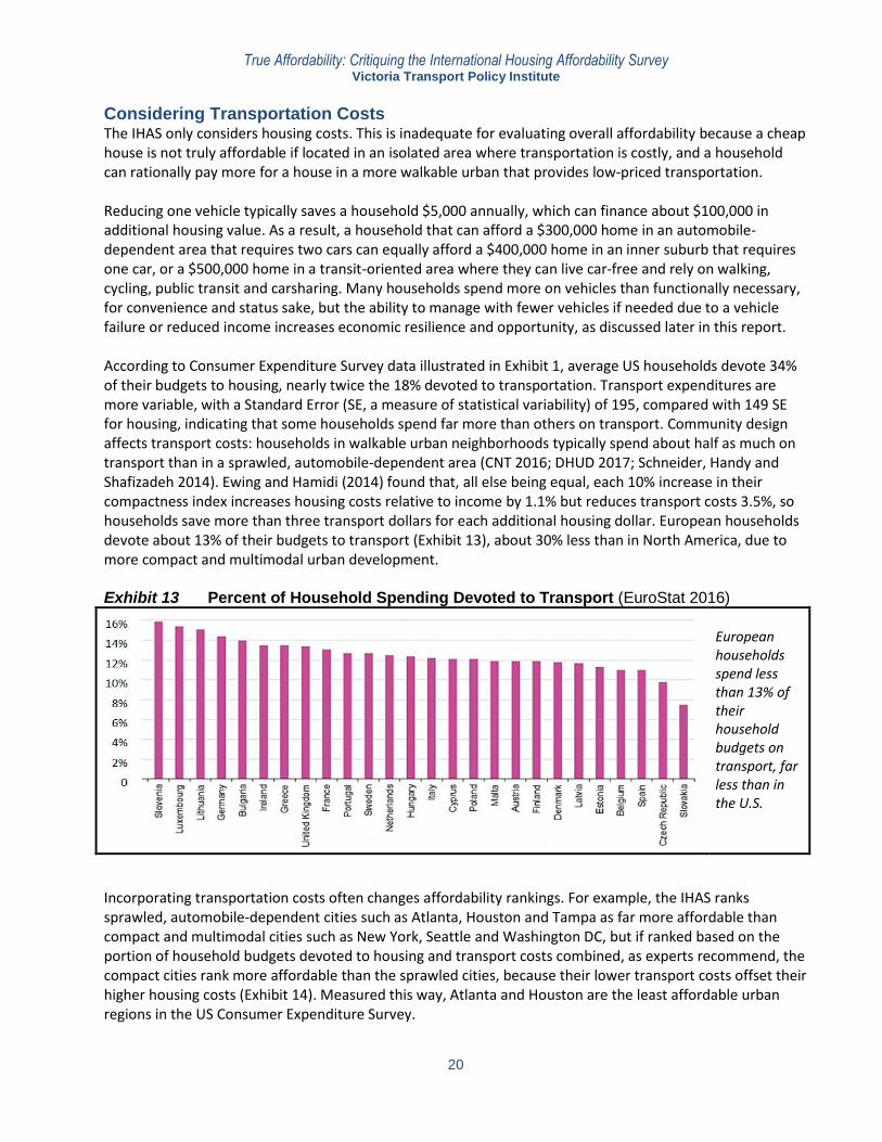
Considering Transportation Costs The IHAS only considers housing costs. This is inadequate for evaluating overall affordability because a cheap house is not truly affordable if located in an isolated area where transportation is costly, and a household can rationally pay more for a house in a more walkable urban that provides low-priced transportation. Reducing one vehicle typically saves a household $5,000 annually, which can finance about $100,000 in additional housing value. As a result, a household that can afford a $300,000 home in an automobile-dependent area that requires two cars can equally afford a $400,000 home in an inner suburb that requires one car, or a $500,000 home in a transit-oriented area where they can live car-free and rely on walking, cycling, public transit and carsharing. Many households spend more on vehicles than functionally necessary, for convenience and status sake, but the ability to manage with fewer vehicles if needed due to a vehicle failure or reduced income increases economic resilience and opportunity, as discussed later in this report. According to Consumer Expenditure Survey data illustrated in Exhibit 1, average US households devote 34% of their budgets to housing, nearly twice the 18% devoted to transportation. Transport expenditures are more variable, with a Standard Error (SE, a measure of statistical variability) of 195, compared with 149 SE for housing, indicating that some households spend far more than others on transport. Community design affects transport costs: households in walkable urban neighborhoods typically spend about half as much on transport than in a sprawled, automobile-dependent area (CNT 2016; DHUD 2017; Schneider, Handy and Shafizadeh 2014). Ewing and Hamidi (2014) found that, all else being equal, each 10% increase in their compactness index increases housing costs relative to income by 1.1% but reduces transport costs 3.5%, so households save more than three transport dollars for each additional housing dollar. European households devote about 13% of their budgets to transport (Exhibit 13), about 30% less than in North America, due to more compact and multimodal urban development. Exhibit 13 Percent of Household Spending Devoted to Transport (EuroStat 2016)

European households spend less than 13% of their household budgets on transport, far less than in the U.S.

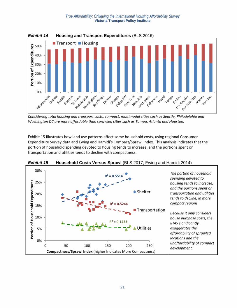
Incorporating transportation costs often changes affordability rankings. For example, the IHAS ranks sprawled, automobile-dependent cities such as Atlanta, Houston and Tampa as far more affordable than compact and multimodal cities such as New York, Seattle and Washington DC, but if ranked based on the portion of household budgets devoted to housing and transport costs combined, as experts recommend, the compact cities rank more affordable than the sprawled cities, because their lower transport costs offset their higher housing costs (Exhibit 14). Measured this way, Atlanta and Houston are the least affordable urban regions in the US Consumer Expenditure Survey.


21

Exhibit 14 Housing and Transport Expenditures (BLS 2016)

Considering total housing and transport costs, compact, multimodal cities such as Seattle, Philadelphia and Washington DC are more affordable than sprawled cities such as Tampa, Atlanta and Houston.

Exhibit 15 illustrates how land use patterns affect some household costs, using regional Consumer Expenditure Survey data and Ewing and Hamidi’s Compact/Sprawl Index. This analysis indicates that the portion of household spending devoted to housing tends to increase, and the portions spent on transportation and utilities tends to decline with compactness. Exhibit 15 Household Costs Versus Sprawl (BLS 2017; Ewing and Hamidi 2014)

The portion of household spending devoted to housing tends to increase, and the portions spent on transportation and utilities tends to decline, in more compact regions. Because it only considers house purchase costs, the IHAS significantly exaggerates the affordability of sprawled locations and the unaffordability of compact development.

0%

10%

20%

30%

40%

50%

Po

rtio

n o

f Ex

pen

dit

ure

s Transport Housing

R² = 0.5514

R² = 0.5244

R² = 0.1433

0%

5%

10%

15%

20%

25%

30%

0 50 100 150 200 250

Po

rtio

n o

f H

ou

seh

old

Exp

end

itu

res

Compactness/Sprawl Index (higher Indicates More Compactness)

Shelter

Transportation

Utilities


22

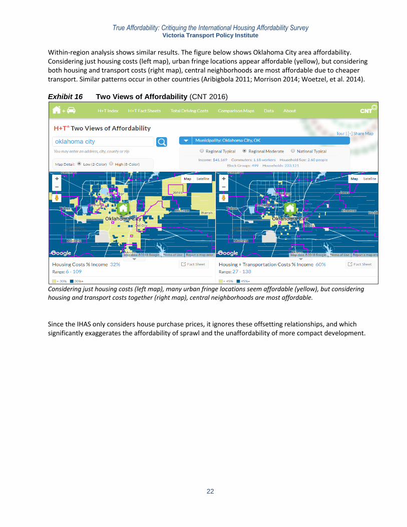
Within-region analysis shows similar results. The figure below shows Oklahoma City area affordability. Considering just housing costs (left map), urban fringe locations appear affordable (yellow), but considering both housing and transport costs (right map), central neighborhoods are most affordable due to cheaper transport. Similar patterns occur in other countries (Aribigbola 2011; Morrison 2014; Woetzel, et al. 2014). Exhibit 16 Two Views of Affordability (CNT 2016)

Considering just housing costs (left map), many urban fringe locations seem affordable (yellow), but considering housing and transport costs together (right map), central neighborhoods are most affordable.

Since the IHAS only considers house purchase prices, it ignores these offsetting relationships, and which significantly exaggerates the affordability of sprawl and the unaffordability of more compact development.


23

Regulatory Impacts The IHAS claims (Table 2) that high housing prices result primarily from urban containment regulations, and allowing urban expansion is the best way to increase affordability. This claim is wrong for several reasons.

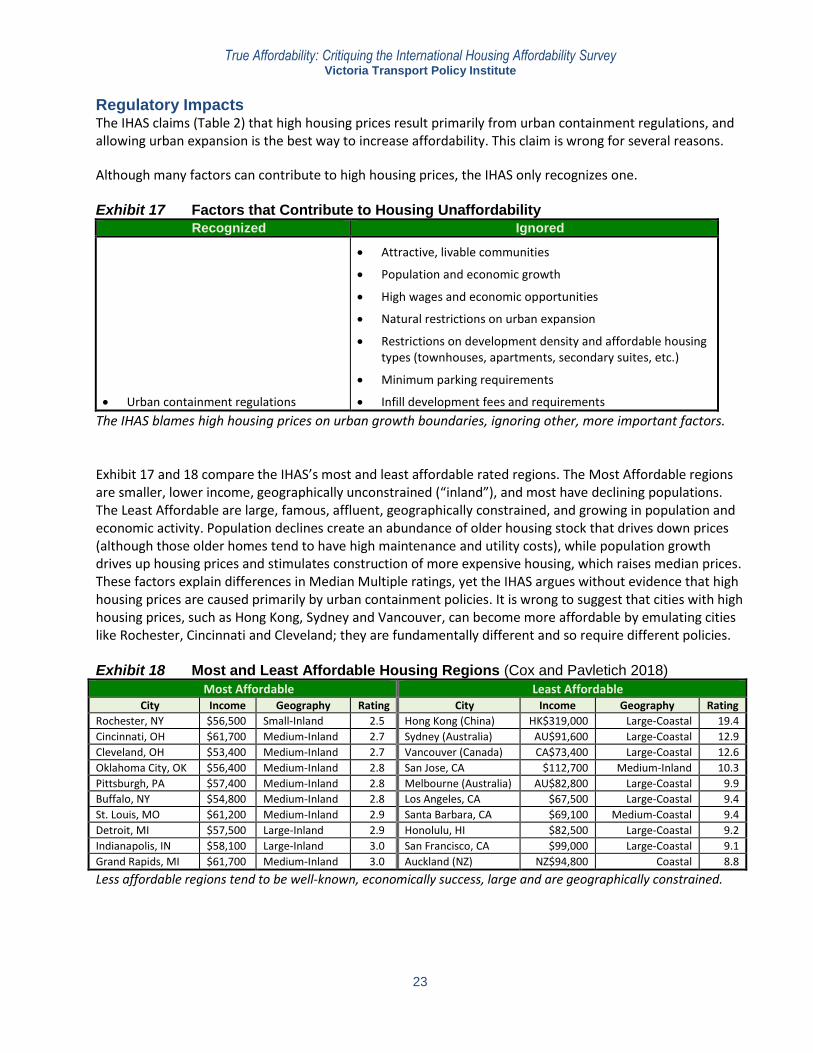
Although many factors can contribute to high housing prices, the IHAS only recognizes one. Exhibit 17 Factors that Contribute to Housing Unaffordability

Recognized Ignored

Urban containment regulations

Attractive, livable communities

Population and economic growth

High wages and economic opportunities

Natural restrictions on urban expansion

Restrictions on development density and affordable housing types (townhouses, apartments, secondary suites, etc.)

Minimum parking requirements

Infill development fees and requirements

The IHAS blames high housing prices on urban growth boundaries, ignoring other, more important factors. Exhibit 17 and 18 compare the IHAS’s most and least affordable rated regions. The Most Affordable regions are smaller, lower income, geographically unconstrained (“inland”), and most have declining populations. The Least Affordable are large, famous, affluent, geographically constrained, and growing in population and economic activity. Population declines create an abundance of older housing stock that drives down prices (although those older homes tend to have high maintenance and utility costs), while population growth drives up housing prices and stimulates construction of more expensive housing, which raises median prices. These factors explain differences in Median Multiple ratings, yet the IHAS argues without evidence that high housing prices are caused primarily by urban containment policies. It is wrong to suggest that cities with high housing prices, such as Hong Kong, Sydney and Vancouver, can become more affordable by emulating cities like Rochester, Cincinnati and Cleveland; they are fundamentally different and so require different policies. Exhibit 18 Most and Least Affordable Housing Regions (Cox and Pavletich 2018)

Most Affordable Least Affordable City Income Geography Rating City Income Geography Rating

Rochester, NY $56,500 Small-Inland 2.5 Hong Kong (China) HK$319,000 Large-Coastal 19.4

Cincinnati, OH $61,700 Medium-Inland 2.7 Sydney (Australia) AU$91,600 Large-Coastal 12.9

Cleveland, OH $53,400 Medium-Inland 2.7 Vancouver (Canada) CA$73,400 Large-Coastal 12.6

Oklahoma City, OK $56,400 Medium-Inland 2.8 San Jose, CA $112,700 Medium-Inland 10.3

Pittsburgh, PA $57,400 Medium-Inland 2.8 Melbourne (Australia) AU$82,800 Large-Coastal 9.9

Buffalo, NY $54,800 Medium-Inland 2.8 Los Angeles, CA $67,500 Large-Coastal 9.4

St. Louis, MO $61,200 Medium-Inland 2.9 Santa Barbara, CA $69,100 Medium-Coastal 9.4

Detroit, MI $57,500 Large-Inland 2.9 Honolulu, HI $82,500 Large-Coastal 9.2

Indianapolis, IN $58,100 Large-Inland 3.0 San Francisco, CA $99,000 Large-Coastal 9.1

Grand Rapids, MI $61,700 Medium-Inland 3.0 Auckland (NZ) NZ$94,800 Coastal 8.8

Less affordable regions tend to be well-known, economically success, large and are geographically constrained.


24

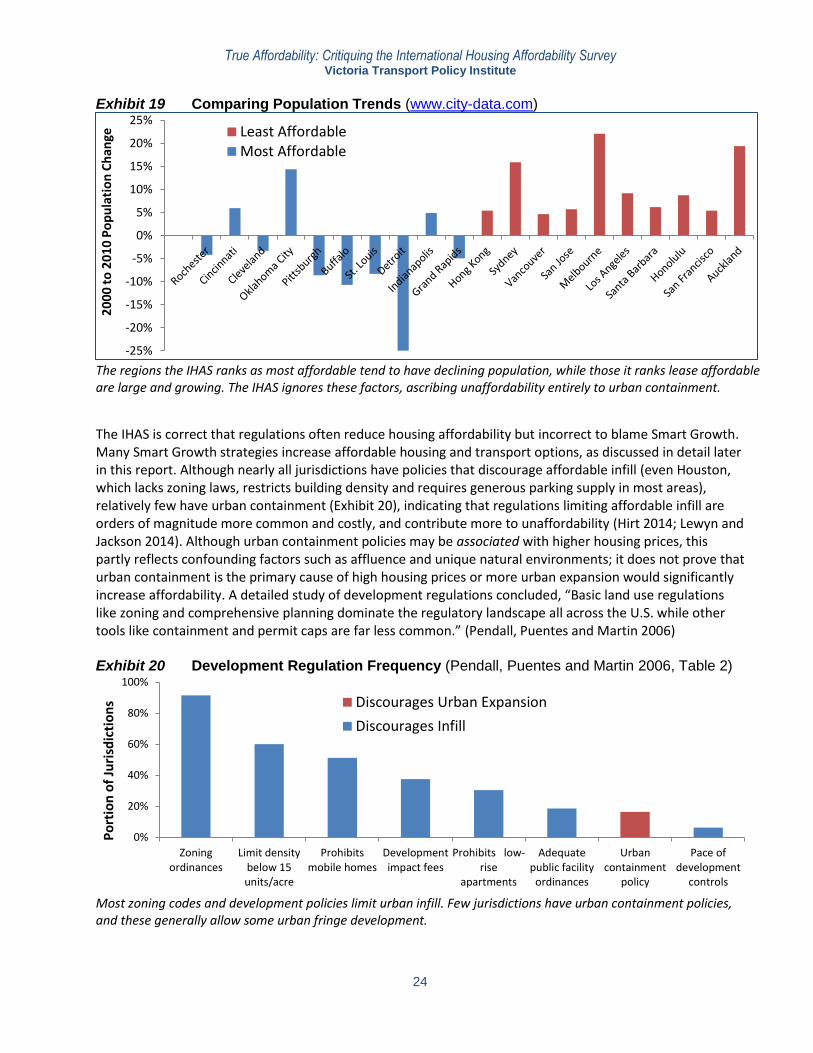
Exhibit 19 Comparing Population Trends (www.city-data.com)

The regions the IHAS ranks as most affordable tend to have declining population, while those it ranks lease affordable are large and growing. The IHAS ignores these factors, ascribing unaffordability entirely to urban containment.

The IHAS is correct that regulations often reduce housing affordability but incorrect to blame Smart Growth. Many Smart Growth strategies increase affordable housing and transport options, as discussed in detail later in this report. Although nearly all jurisdictions have policies that discourage affordable infill (even Houston, which lacks zoning laws, restricts building density and requires generous parking supply in most areas), relatively few have urban containment (Exhibit 20), indicating that regulations limiting affordable infill are orders of magnitude more common and costly, and contribute more to unaffordability (Hirt 2014; Lewyn and Jackson 2014). Although urban containment policies may be associated with higher housing prices, this partly reflects confounding factors such as affluence and unique natural environments; it does not prove that urban containment is the primary cause of high housing prices or more urban expansion would significantly increase affordability. A detailed study of development regulations concluded, “Basic land use regulations like zoning and comprehensive planning dominate the regulatory landscape all across the U.S. while other tools like containment and permit caps are far less common.” (Pendall, Puentes and Martin 2006) Exhibit 20 Development Regulation Frequency (Pendall, Puentes and Martin 2006, Table 2)

Most zoning codes and development policies limit urban infill. Few jurisdictions have urban containment policies, and these generally allow some urban fringe development.

-25%

-20%

-15%

-10%

-5%

0%

5%

10%

15%

20%

25%2

00

0 t

o 2

01

0 P

op

ula

tio

n C

han

ge

Least AffordableMost Affordable

0%

20%

40%

60%

80%

100%

Zoningordinances

Limit densitybelow 15units/acre

Prohibitsmobile homes

Developmentimpact fees

Prohibits low-rise

apartments

Adequatepublic facility

ordinances

Urbancontainment

policy

Pace ofdevelopment

controls

Po

rtio

n o

f Ju

risd

icti

on

s Discourages Urban Expansion

Discourages Infill

http://www.city-data.com/


25

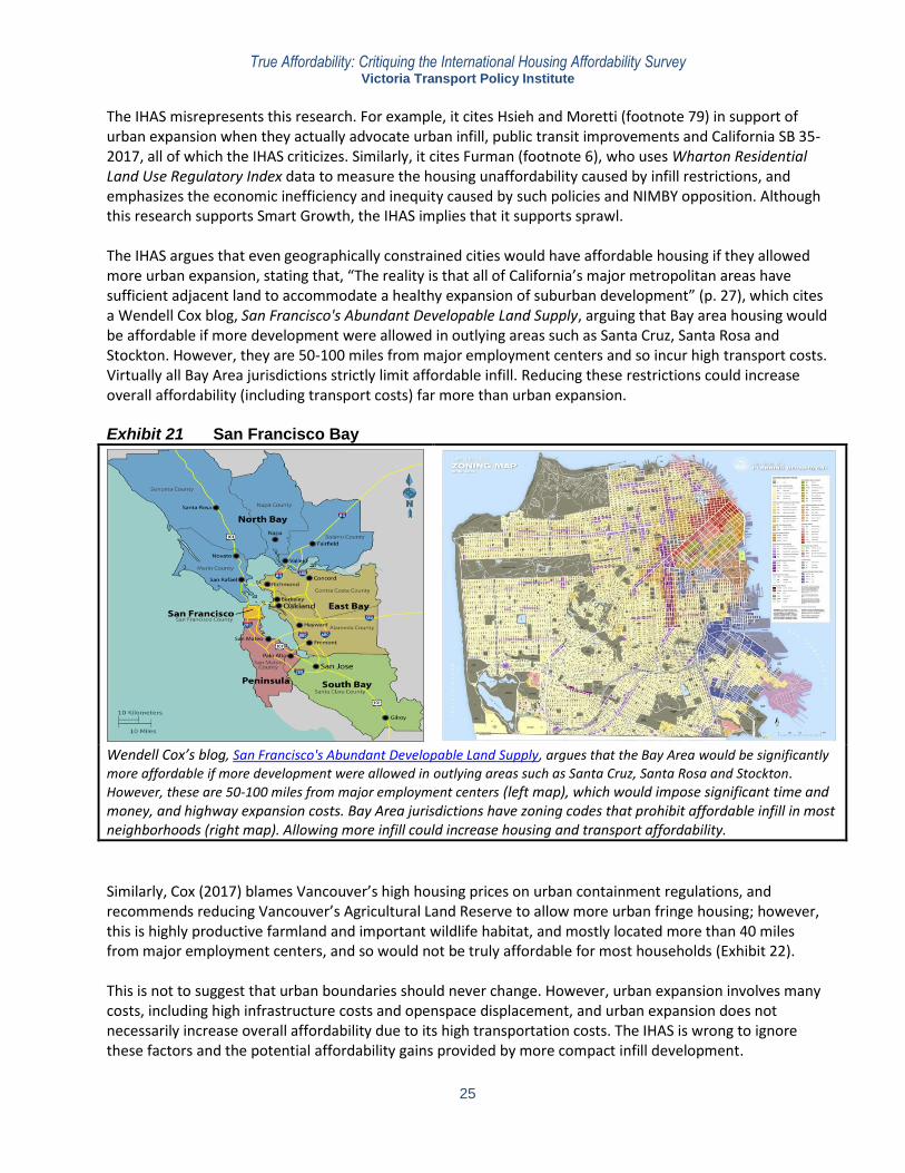
The IHAS misrepresents this research. For example, it cites Hsieh and Moretti (footnote 79) in support of urban expansion when they actually advocate urban infill, public transit improvements and California SB 35-2017, all of which the IHAS criticizes. Similarly, it cites Furman (footnote 6), who uses Wharton Residential Land Use Regulatory Index data to measure the housing unaffordability caused by infill restrictions, and emphasizes the economic inefficiency and inequity caused by such policies and NIMBY opposition. Although this research supports Smart Growth, the IHAS implies that it supports sprawl. The IHAS argues that even geographically constrained cities would have affordable housing if they allowed more urban expansion, stating that, “The reality is that all of California’s major metropolitan areas have sufficient adjacent land to accommodate a healthy expansion of suburban development” (p. 27), which cites a Wendell Cox blog, San Francisco's Abundant Developable Land Supply, arguing that Bay area housing would be affordable if more development were allowed in outlying areas such as Santa Cruz, Santa Rosa and Stockton. However, they are 50-100 miles from major employment centers and so incur high transport costs. Virtually all Bay Area jurisdictions strictly limit affordable infill. Reducing these restrictions could increase overall affordability (including transport costs) far more than urban expansion. Exhibit 21 San Francisco Bay

Wendell Cox’s blog, San Francisco's Abundant Developable Land Supply, argues that the Bay Area would be significantly

more affordable if more development were allowed in outlying areas such as Santa Cruz, Santa Rosa and Stockton.

However, these are 50-100 miles from major employment centers (left map), which would impose significant time and money, and highway expansion costs. Bay Area jurisdictions have zoning codes that prohibit affordable infill in most neighborhoods (right map). Allowing more infill could increase housing and transport affordability.

Similarly, Cox (2017) blames Vancouver’s high housing prices on urban containment regulations, and recommends reducing Vancouver’s Agricultural Land Reserve to allow more urban fringe housing; however, this is highly productive farmland and important wildlife habitat, and mostly located more than 40 miles from major employment centers, and so would not be truly affordable for most households (Exhibit 22). This is not to suggest that urban boundaries should never change. However, urban expansion involves many costs, including high infrastructure costs and openspace displacement, and urban expansion does not necessarily increase overall affordability due to its high transportation costs. The IHAS is wrong to ignore these factors and the potential affordability gains provided by more compact infill development.

http://www.newgeography.com/content/005773-san-franciscos-abundant-developable-land-supply


26

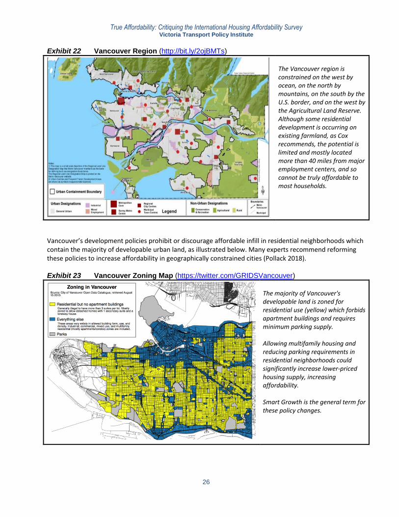
Exhibit 22 Vancouver Region (http://bit.ly/2ojBMTs)

The Vancouver region is constrained on the west by ocean, on the north by mountains, on the south by the U.S. border, and on the west by the Agricultural Land Reserve. Although some residential development is occurring on existing farmland, as Cox recommends, the potential is limited and mostly located more than 40 miles from major employment centers, and so cannot be truly affordable to most households.

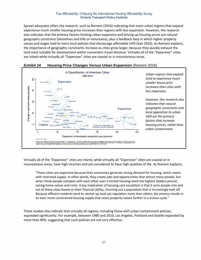
Vancouver’s development policies prohibit or discourage affordable infill in residential neighborhoods which contain the majority of developable urban land, as illustrated below. Many experts recommend reforming these policies to increase affordability in geographically constrained cities (Pollack 2018). Exhibit 23 Vancouver Zoning Map (https://twitter.com/GRIDSVancouver)

The majority of Vancouver's developable land is zoned for residential use (yellow) which forbids apartment buildings and requires minimum parking supply. Allowing multifamily housing and reducing parking requirements in residential neighborhoods could significantly increase lower-priced housing supply, increasing affordability. Smart Growth is the general term for these policy changes.

http://bit.ly/2ojBMTs

https://twitter.com/GRIDSVancouver


27

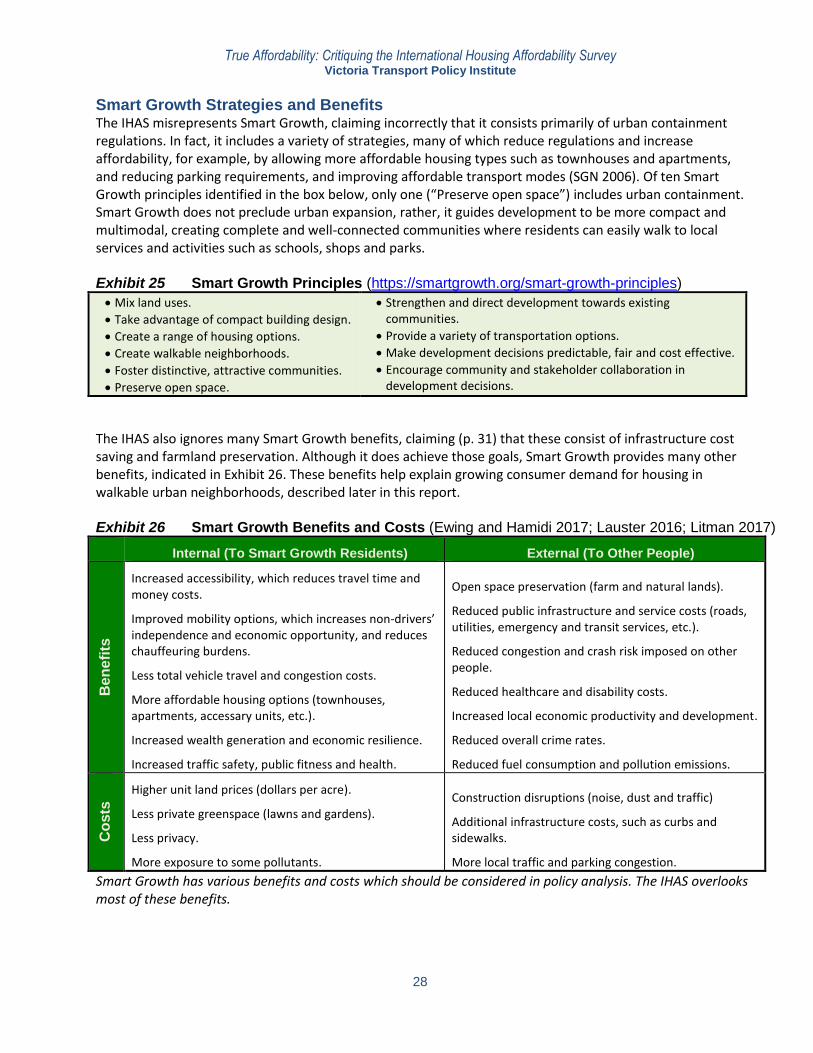
Sprawl advocates often cite research, such as Romem (2016) indicating that more urban regions that expand experience much smaller housing price increases than regions with less expansion. However, the research also indicates that the primary factors limiting urban expansion and driving up housing prices are natural geographic constrains (shorelines and hills or mountains), plus a feedback loop in which higher property values and wages lead to more local policies that discourage affordable infill (Saiz 2010). As Romem explains, the importance of geographic constraints increase as cities grow larger, because they quickly exhaust the land most suitable for development within convenient travel distance. Virtually all of the “Expansive” cities are inland while virtually all “Expensive” cities are coastal or in mountainous areas. Exhibit 24 Housing Price Changes Versus Urban Expansion (Romem 2016)

Urban regions that expand tend to experience much smaller house price increases than cities with less expansion. However, this research also indicates that natural geographic constraints and local opposition to urban infill are the primary factors that increase housing prices, rather than urban containment.

Virtually all of the “Expansive” cities are inland, while virtually all “Expensive” cities are coastal or in mountainous areas, have high incomes and are considered to have high qualities of life. As Romem explains,

“These cities are expensive because their economies generate strong demand for housing, which meets with restricted supply. In other words, they create jobs and opportunities that attract many people, but when these people compete with each other over a limited housing stock the highest bidders prevail, raising home values and rents. A key implication of housing cost escalation is that it sorts people into and out of these cities based on their financial ability, churning out a population that is increasingly well off. Because affluent residents tend to ratchet up land use regulation more than others, the process results in an even more constrained housing supply that raises property values further in a vicious cycle.”

These studies also indicate that virtually all regions, including those with urban containment policies, expanded significantly. For example, between 1980 and 2010, Los Angeles, Portland and Seattle expanded by more than 40%, suggesting that such policies are not very effective.


28

Smart Growth Strategies and Benefits The IHAS misrepresents Smart Growth, claiming incorrectly that it consists primarily of urban containment regulations. In fact, it includes a variety of strategies, many of which reduce regulations and increase affordability, for example, by allowing more affordable housing types such as townhouses and apartments, and reducing parking requirements, and improving affordable transport modes (SGN 2006). Of ten Smart Growth principles identified in the box below, only one (“Preserve open space”) includes urban containment. Smart Growth does not preclude urban expansion, rather, it guides development to be more compact and multimodal, creating complete and well-connected communities where residents can easily walk to local services and activities such as schools, shops and parks. Exhibit 25 Smart Growth Principles (https://smartgrowth.org/smart-growth-principles)

Mix land uses.

Take advantage of compact building design.

Create a range of housing options.

Create walkable neighborhoods.

Foster distinctive, attractive communities.

Preserve open space.

Strengthen and direct development towards existing communities.

Provide a variety of transportation options.

Make development decisions predictable, fair and cost effective.

Encourage community and stakeholder collaboration in development decisions.

The IHAS also ignores many Smart Growth benefits, claiming (p. 31) that these consist of infrastructure cost saving and farmland preservation. Although it does achieve those goals, Smart Growth provides many other benefits, indicated in Exhibit 26. These benefits help explain growing consumer demand for housing in walkable urban neighborhoods, described later in this report. Exhibit 26 Smart Growth Benefits and Costs (Ewing and Hamidi 2017; Lauster 2016; Litman 2017)

Internal (To Smart Growth Residents) External (To Other People)

Be

ne

fits

Increased accessibility, which reduces travel time and money costs.

Improved mobility options, which increases non-drivers’ independence and economic opportunity, and reduces chauffeuring burdens.

Less total vehicle travel and congestion costs.

More affordable housing options (townhouses, apartments, accessary units, etc.).

Increased wealth generation and economic resilience.

Increased traffic safety, public fitness and health.

Open space preservation (farm and natural lands).

Reduced public infrastructure and service costs (roads, utilities, emergency and transit services, etc.).

Reduced congestion and crash risk imposed on other people.

Reduced healthcare and disability costs.

Increased local economic productivity and development.

Reduced overall crime rates.

Reduced fuel consumption and pollution emissions.

Co

sts

Higher unit land prices (dollars per acre).

Less private greenspace (lawns and gardens).

Less privacy.

More exposure to some pollutants.

Construction disruptions (noise, dust and traffic)

Additional infrastructure costs, such as curbs and sidewalks.

More local traffic and parking congestion.

Smart Growth has various benefits and costs which should be considered in policy analysis. The IHAS overlooks most of these benefits.

https://smartgrowth.org/smart-growth-principles


29

The following sections describe Smart Growth benefits in more detail. Improved Accessibility and Transportation Cost Savings Accessibility refers to people’s ability to reach activities and destinations (Brookings Institution 2016). More compact and multimodal development tends to improve overall accessibility, particularly for non-drivers, by reducing distances between destinations and improving travel options. As a result, living in a central urban neighborhood increases the variety of services and activities available within a given time and financial budget, and additionally provides travel time and travel cost savings. These savings and benefits are particularly important for people who cannot, should not or prefer not to drive. Households located in more accessible areas own fewer vehicles, drive less, and spend less on transportation than they would in more automobile-dependent areas (CNT 2016). Of course, travel demands are diverse and not always rational. Many households own more vehicles than functionally necessary, for convenience and status sake. However, the ability to survive comfortably without a vehicle, and to reduce transportation costs when necessary, provides large user benefits. By reducing per capita vehicle travel it also reduces traffic problems including congestion, parking, accident and pollution costs imposed on a community. The IHAS argues that compact development increases traffic congestion and travel times. There is some truth and much inaccuracy in these claims. Compact development tends to increase congestion intensity but reduces per capita congestion costs by reducing total vehicle travel and per capita congestion delays. For example, according to the 2015 Urban Mobility Scorecard (TTI 2015), the New York region has a 1.34 Travel Time Index, slightly higher than Houston’s 1.33, indicating that New York area drivers experience greater peak period speed reductions, but Houston commuters average 48 annual hours of congestion delay (61 annual delay hours per auto commuter times 79% auto mode share), much higher than the 37 annual hours of delay in New York (74 annual delay hours per auto commuter times 50% auto mode share). Commute duration tends to increase with city size and transit mode share (since transit trips take longer, door-to-door, than automobile trips) which explains why Boston, Chicago and New York have longer duration commutes than Atlanta, Houston and Phoenix. However, these longer duration commute trips are often worthwhile and preferred by users. Non-auto commuting provides financial savings that are often worth the incremental time. For example, if a commuter can save several dollars per day in vehicle expenses or parking fees, values the additional exercise, or considers non-auto modes less stressful than driving, the additional time spent commuting may be cost effective. Of course, travel needs and preference vary; living in a multimodal location allows commuters to choose the best option for each trip. For example, driving when they have money or after-work errands, and using other modes when their budgets are tight, when they want exercise, or to allow safe and legal after-work drinking. Only about 20% of personal travel is for commuting, so even if compact development increases the journey to work duration it can reduce total travel time burdens. This includes the time required for personal errands and chauffeuring non-drivers. In virtually all urban regions, central locations significantly improve accessibility and reduce total travel times. A major study in Phoenix, Arizona found less intense congestion and reduced per capita travel times in older neighborhoods with more compact and mixed development, more connected streets, better walking conditions and better public transit services than in newer, lower-density, automobile-dependent suburbs. This is partly because residents drive less and have more route options (Kuzmyak 2012).


30

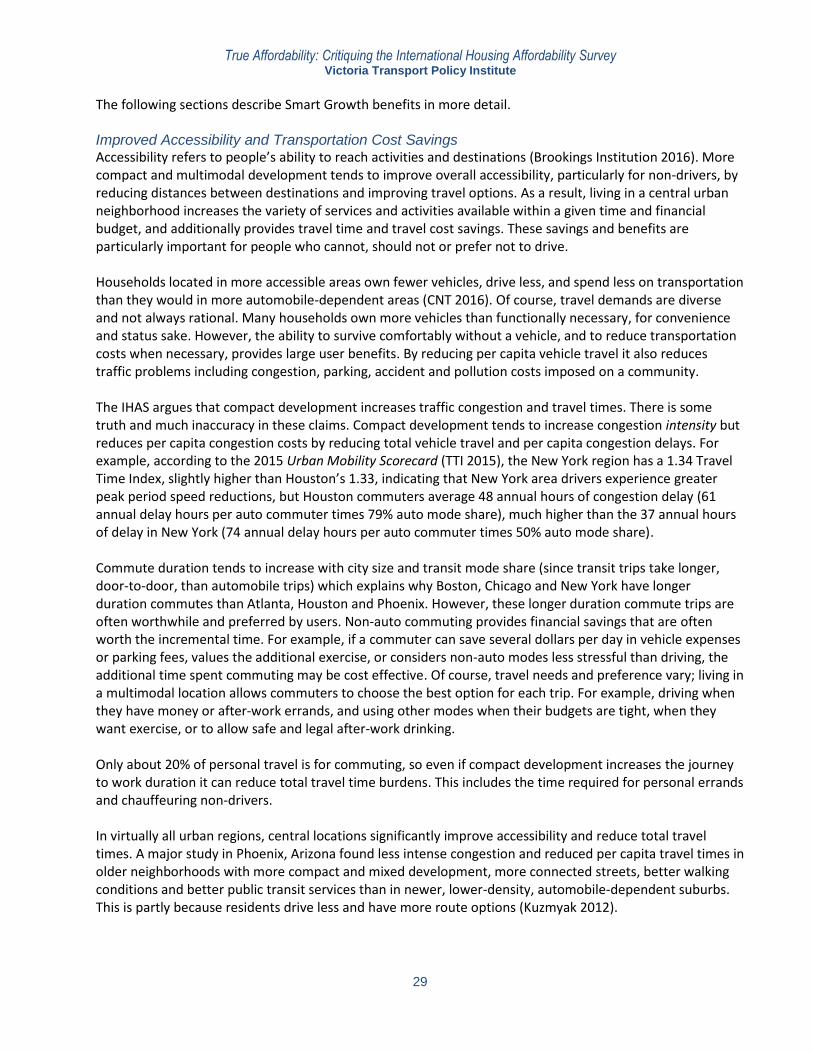
Exhibit 27 shows the Chicago regions’ 40-minute job access. Although driving can generally access more jobs than transit, central area transit users can access far more jobs than urban fringe motorists, and central areas jobs usually pay higher wages, indicating the large economic benefits of central location. Exhibit 27 Transit and Driving 40-minute Jobs Access (http://urbanaccessibility.com)

Although driving (left map) can access more regional jobs than transit (right map), central area transit commuters can access more jobs than urban fringe auto commuters, and city center jobs tend to pay better. This indicates central locations provide economic benefits, particularly for workers who cannot, should not, or prefer not to drive.

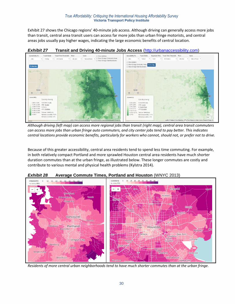
Because of this greater accessibility, central area residents tend to spend less time commuting. For example, in both relatively compact Portland and more sprawled Houston central area residents have much shorter duration commutes than at the urban fringe, as illustrated below. These longer commutes are costly and contribute to various mental and physical health problems (Kylstra 2014). Exhibit 28 Average Commute Times, Portland and Houston (WNYC 2013)

Residents of more central urban neighborhoods tend to have much shorter commutes than at the urban fringe.

http://urbanaccessibility.com/


31

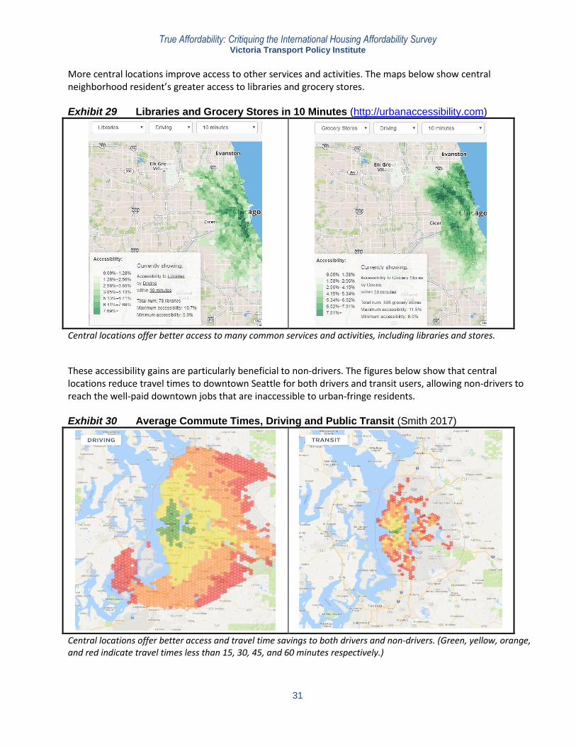
More central locations improve access to other services and activities. The maps below show central neighborhood resident’s greater access to libraries and grocery stores. Exhibit 29 Libraries and Grocery Stores in 10 Minutes (http://urbanaccessibility.com)

Central locations offer better access to many common services and activities, including libraries and stores.

These accessibility gains are particularly beneficial to non-drivers. The figures below show that central locations reduce travel times to downtown Seattle for both drivers and transit users, allowing non-drivers to reach the well-paid downtown jobs that are inaccessible to urban-fringe residents. Exhibit 30 Average Commute Times, Driving and Public Transit (Smith 2017)

Central locations offer better access and travel time savings to both drivers and non-drivers. (Green, yellow, orange, and red indicate travel times less than 15, 30, 45, and 60 minutes respectively.)

http://urbanaccessibility.com/


32

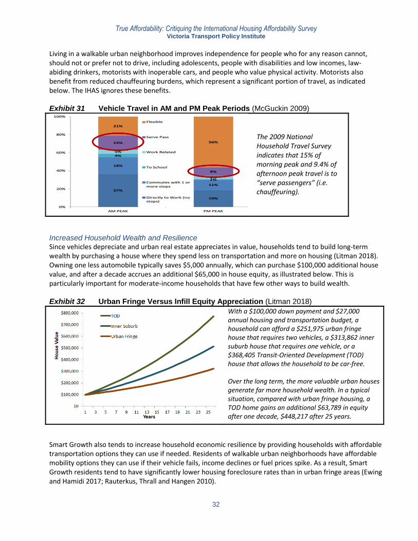
Living in a walkable urban neighborhood improves independence for people who for any reason cannot, should not or prefer not to drive, including adolescents, people with disabilities and low incomes, law-abiding drinkers, motorists with inoperable cars, and people who value physical activity. Motorists also benefit from reduced chauffeuring burdens, which represent a significant portion of travel, as indicated below. The IHAS ignores these benefits. Exhibit 31 Vehicle Travel in AM and PM Peak Periods (McGuckin 2009)

The 2009 National Household Travel Survey indicates that 15% of morning peak and 9.4% of afternoon peak travel is to “serve passengers” (i.e. chauffeuring).

Increased Household Wealth and Resilience Since vehicles depreciate and urban real estate appreciates in value, households tend to build long-term wealth by purchasing a house where they spend less on transportation and more on housing (Litman 2018). Owning one less automobile typically saves $5,000 annually, which can purchase $100,000 additional house value, and after a decade accrues an additional $65,000 in house equity, as illustrated below. This is particularly important for moderate-income households that have few other ways to build wealth. Exhibit 32 Urban Fringe Versus Infill Equity Appreciation (Litman 2018)

With a $100,000 down payment and $27,000 annual housing and transportation budget, a household can afford a $251,975 urban fringe house that requires two vehicles, a $313,862 inner suburb house that requires one vehicle, or a $368,405 Transit-Oriented Development (TOD) house that allows the household to be car-free. Over the long term, the more valuable urban houses generate far more household wealth. In a typical situation, compared with urban fringe housing, a TOD home gains an additional $63,789 in equity after one decade, $448,217 after 25 years.

Smart Growth also tends to increase household economic resilience by providing households with affordable transportation options they can use if needed. Residents of walkable urban neighborhoods have affordable mobility options they can use if their vehicle fails, income declines or fuel prices spike. As a result, Smart Growth residents tend to have significantly lower housing foreclosure rates than in urban fringe areas (Ewing and Hamidi 2017; Rauterkus, Thrall and Hangen 2010).


33

Traffic Safety Various studies indicate that more compact development significantly increases traffic safety, often reducing fatality rates by 50-75% (Welle, et al. 2018). Ewing and Hamidi (2014) found that a 10% reduction in their Sprawl Index reduces per capita crash fatality rates 13.8%. Garrick and Marshall (2011) found that more compact and multi-modal communities have a third the traffic fatality rates as automobile dependent areas, and that sprawl-inducing practices, such as separated land uses and higher roadway design speeds increase crash rates by increasing vehicle mileage and speeds. Exhibit 33 illustrates one study’s results. Exhibit 33 Annual Traffic Death Rate (Ewing, Schieber and Zegeer 2003)

Of 280 U.S. counties analyzed, the ten with the lowest sprawl rating have about a quarter the per capita annual traffic fatality rates of the most sprawled counties.

Public Fitness and Health Many studies find that Smart Growth tends to increase physical fitness and health (Ewing and Hamidi 2014). Although there are many ways to exercise, most require special time, expense and effort, which discourages their use, particularly by sedentary and overweight people. One of the most effective ways to increase physical fitness in a community is to improve walking and cycling conditions, and encourage use of these modes for both recreation and utilitarian purposes (CDC 2010). In a study of 14 international cities, Sallis, et al. (2016) found that, controlling other factors, residential and intersection density, public transport density and number of parks were significantly, positively related to physical activity. Compared with the least activity-friendly areas, residents in the most active neighborhoods gained 68-89 min/week, which represents 45–59% of recommended physical activity targets. Using sophisticated statistical analysis that accounts for various demographic and economic factors, Ewing, et al. (2014) found that Smart Growth is associated with reduced obesity and associated health problems. Ewing and Hamidi (2014) found that doubling their Sprawl Index increased life expectancy approximately 4%, which translates into a three-year average gain between the least and more compact counties. A major UK study found that, accounting for other demographic factors, incremental increases in neighborhood walkability are associated with significantly reduced blood pressure and hypertension risk (Sarkar, Webster and Gallacher 2018). Frederick, Riggs and Gilderbloom (2017), found that, accounting for various demographic factors, cities with lower automobile commuter mode share (an indicator of Smart Growth) have more positive public health outcomes including healthier behaviors reported in the Gallup/Healthway’s Well-Being Index, less sedentary living and obesity reported in the Center for Disease Control’s Diabetes Interactive Atlas, and higher birth weights (an indicator of infant health). Long duration automobile commutes contribute to mental and physical health problems (Kylstra 2014; MacMillian 2015).


34

Economic Productivity and Opportunity One of the IHAS’s most inaccurate claims is that sprawl increases economic productivity and opportunity (p. 29 & 34). Good research indicates the opposite. Extensive research shows that more compact and multi-modal development tends to increase economic productivity through economies of agglomeration (Melo, Graham and Noland 2009). Other research indicates that physically, economically and socially disadvantaged people have more independence, higher wages and greater economic opportunities if they live in more compact and multimodal neighborhoods because this improves their access to education, employment, positive role models, and money saving opportunities such affordable transport options and discount stores (Ewing, et al. 2016; Levy, McDade and Dumlao 2010). These benefits are particularly large for non-drivers (Kneebone and Holmes 2015). Economists Hsieh and Moretti (2017) estimate that allowing more affordable infill development in highly productive cities (Boston, New York, Seattle, San Francisco and Washington DC) would significantly increase total US productivity and economic opportunity for disadvantaged workers; the IHAS cites this research inaccurately as supporting sprawl; in fact, the authors specifically recommend more affordable infill and improve public transit services. Ewing and Hamidi (2014 and 2017) found that each 10% increase in their Smart Growth index is associated with a 4.1% increase in residents’ upward mobility (the probability a child born in the lowest income quintile will reach the top quintile by age 30). The IHAS argues that because most workers commute by automobile, and workers with automobiles tend to earn more money, disadvantaged people benefit from automobile-oriented planning and are harmed by multimodal planning. However, this misrepresents the issues. Many disadvantaged people cannot or should not drive due to disabilities, poverty or lack of a driver’s license, and so benefit significantly from improved transport options. Even those who drive benefit from having affordable options that they can use to save money or as a backup when their car is unavailable (Agrawal, et al. 2011). A sophisticated panel study by Smart and Klein (2015) found that, although automobile access increases disadvantaged workers’ hours and incomes, their additional vehicle expenses exceed their average income gains. Improving affordable modes (walking, bicycling and public transit) increases disadvantaged residents’ economic opportunity, with lower costs and therefore greater net benefits than automobile transport (CTS 2010; Sadler and Wampler 2013). Exhibit 34 indicates affordable housing and transportation budgets by income class, assuming that these goods should total no more than 45% of household spending, and urban fringe area motorists spend $5,000 annually per vehicle. By this standard, first- and second-income quintile households can only afford to own a motor vehicle if their total housing costs (rents or mortgages, maintenance, utilities and taxes) are less than $526 and $962 respectively, and owning two cars strains the budgets of households that spend more than $954 per month on housing. This indicates that urban-fringe housing is unaffordable to most low- and moderate-income households. Exhibit 34 Housing and Transportation Budget by Income Class (BLS 2016)

First Second Third Fourth Fifth

Monthly income $2,095 $3,064 $3,972 $5,409 $9,352

Monthly housing and transport budget $943 $1,379 $1,787 $2,434 $4,208

Maximum monthly rent with one car $526 $962 $1,371 $2,018 $3,792

Maximum monthly rent with two cars $109 $546 $954 $1,601 $3,375

First- and second-income quintile households can only afford a car if their total housing costs (including maintenance, utilities, taxes and insurance) are low, and even third income quintile households are often financially strained by the costs of two cars.


35

Consumer Preferences The IHAS argues that consumers demand urban-fringe housing, and so are harmed by policies that encourage compact infill. These arguments are largely incorrect and outdated. Given unlimited resources most people would probably prefer a detached home, or even a castle, but the National Association of Realtor’s National Community and Transportation Preference Survey (NAR 2017), indicates that a growing majority of home buyers prefer an attached house (townhouse or apartments) in a walkable urban neighborhood over a detached house that requires a longer commute and driving to shops, as illustrated below. Most respondents like walking (80%), driving (73%), about half like bicycling, more than a third (38%) like public transit travel, and nearly 60% report driving due to inadequate alternatives. Younger people are much more likely to prefer walkable neighborhoods, bicycling and transit travel, suggesting that their demand will increase. Walkable community residents are also more satisfied with their quality of life. Exhibit 35 Housing Preference Trends (NAR 2017)

The National Association of Realtors survey indicates a growing preference for living in walkable urban neighborhoods even if that requires attached housing (apartment or townhouse). The IHAS ignores this research, claiming that most households still prefer automobile-dependent sprawl.

The survey also investigated the types of new housing needed to serve unmet demands. Only 10% of attached home residents would prefer a detached house in an automobile-dependent neighborhood, but more than twice as many (21%) detached home residents would prefer an attached house in a walkable urban neighborhood, as indicated below. Since there are about five times as many detached as attached housing units in the U.S., this indicates about ten times more latent demand for compact housing in walkable neighborhoods than detached housing in sprawled, automobile-oriented areas. The IHAS is wrong to claim that significantly more urban fringe development is needed to serve future consumer demands. Rather, Smart Growth policies that allow more affordable infill in walkable neighborhoods best respond to demands. Exhibit 36 What Housing Type is Needed? (NAR 2017)

The survey found that only 10% of attached home residents would prefer a detached house in a conventional neighborhood, but 21% of detached home residents would prefer a townhouse or apartment in a walkable urban neighborhood. This indicates a significant shortage of Smart Growth housing.


36

Critiquing Specific Claims The following table critiques some of the IHAS’s specific claims. Exhibit 37 Claims and Responses

IHAS Claim Critique

“Virtually all the severely unaffordable major housing markets covered in the Demographia International Housing Affordability Survey have restrictive land use regulation, usually urban containment policy.” (p. 3, and similar claims on pages 7 and 30)

Regulations that discourage affordable urban infill, such as restrictions on attached housing and minimum parking requirements, are far more common than urban containment policies. (Pendall, Puentes and 2006)

“Urban containment are the most important of more restrictive land use regulation…and is an important strategy of “growth management” or "smart growth.” (Table 2)

Smart Growth involves many strategies, many of which involve reducing regulations and increase affordability. Urban containment is actually uncommon (Lewyn and Jackson, 2014).

“Urban containment policy has been associated with more expensive housing, which has lowered the standard of living, increased poverty and stunted economic growth.”

More compact development tends to increase productivity, incomes and economic opportunity, and reduces poverty (Ewing, et al. 2016; Hsieh and Moretti 2017).

“…the lower population densities typical of liberal markets are associated with less intense traffic congestion and shorter average work trip journey times.” (p. 7)

Urban fringe residents actually experience more congestion delay, longer duration commutes, and more total time travelling than central area residents (WNYC 2013).

“Some analysts claim that urban fringe development is impossible because of topographic barriers. The reality is that all of California's major metropolitan areas have sufficient adjacent land to accommodate a healthy expansion of suburban development.” (p. 27)

“Some analysts” are not identified (it may be me). The second sentence cites Cox’s blog which cites a 1997 report indicating that the greater San Francisco region has 1,500-4,300 square miles of developable land, but that is mostly in distant areas where residents would bear high travel costs.

“Worsening housing affordability and its adverse impact on the declining standard of living threaten one of the greatest human advances in history – the democratization of prosperity.” (p. 28)

Compact and multimodal development tends to increase disadvantaged people’s economic opportunities and resilience, resulting in improved economic outcomes (Ewing, et al. 2016)

Example comparing housing costs in San Francisco and Atlanta metropolitan areas (p. 28)

This example ignores the higher transportation costs and traffic risks in Atlanta. Considering transport as well as housing costs, Atlanta is actually less affordable than San Francisco.

“Contrary to expectations that higher densities would lower land costs and preserve housing affordability, house prices have skyrocketed inside the UGBs.” (p. 30)

This is a false example. The areas cited (the San Francisco region) continues to restrict infill in most urban neighborhoods, so densities have not significantly increased.

“A principal purpose of urban containment policy is to stop the spatial expansion (pejoratively called “urban sprawl”) of urban areas. This justified by various rationales, such as the cost of infrastructure for new development, preservation of agricultural land and providing mass transit service throughout the urban form.” (p. 31).

This is an incomplete description of sprawl costs and justifications for Smart Growth policies. As discussed in this report, more compact and multimodal development provides many direct and indirect benefits, and many households want to live in walkable urban neighborhoods but cannot due to inadequate supply (Ewing and Hamidi 2017; Litman 2017)

“The mass transit rationale for urban containment is based on an archaic, pre-automobile, early 20

th century perception of the city

as mono-centric, organized around a central business district (CBD) assumed to contain most of the employment.” (p. 32)

This ignores many benefits of high quality transit and transit-oriented development (TOD), which can improve access to jobs, and large savings and benefits, particularly for non-drivers. Many TOD residents have better job without a car than urban fringe residents have with a car.

“…even with torrid high-density building rates in urban cores, such as Vancouver, Toronto and Sydney, housing affordability has worsened.” (p. 33)

Yes, because that densification is only occurring in the core. Affordability requires more affordable infill in residential neighborhoods where land prices are lower.

“…a growing body of research associates strong land use regulation with diminished economic growth.”

This links to Cox’s blog which cites Hseih and Moretti, who actually conclude the opposite: that restriction on infill and inadequate public transit reduce economic development.

The IHAS makes many inaccurate claims.


37

The IHAS ignores evidence that more infill development can increase affordability. For example, in 2017, after the Seattle region developed approximately 20,000 new apartment units, vacancy rates increased and rents declined, ending a decade of price increases (Takeo 2018); with more than 60,000 more units currently under development prices should decline further (Richter 2018). Seattle’s Housing Affordability and Livability Agenda makes moderate-priced residential infill an official policy goal, which should further increase housing supply and reduce prices (CoS 2016; Seattle Weekly 2017). Similarly, Lewyn (2017, Table 3.3) found that Brooklyn, NY rents declined after rental apartment supply increased, in contrast to rent increases in other cities including Manhattan, Raleigh and Austin. Despite similar population growth rates, Montreal housing prices are about half those in Vancouver due to long-standing policies that allow mid-rise apartment development in most neighborhoods (Vallee 2015). Even if new units are initially too expensive for lower-income households, they increase affordability through filtering (occupants of lower-priced housing moving into new higher priced units), and as the new units depreciate, which typically averages about 1% annually if supply grows slowly and up to 3% where supply grows rapidly (Hertz 2015). The IHAS criticizes urban containment policies as “draconian,” although most of urban regions the IHAS criticizes actually experience significant expansion (Angel, et al. 2016). For example, 86% of Toronto’s 2001 to 2011 growth occurred on urban-fringe greenfields (Burchfield and Kramer 2015), indicating that these regulations are actually weak. This indicates bias: the IHAS calls even modest restrictions on expansion “draconian,” but ignores much more frequent and costly restrictions on affordable infill, such a density restrictions, prohibitions on multifamily housing, and costly parking requirements in walkable urban neighborhoods, which significantly reduce affordability. The IHAS is particularly wrong to imply that Smart Growth policies harm disadvantaged people. Compared with automobile-dependent sprawl, affordable infill development provides many advantages to physically, economically and socially disadvantaged people, as summarized below. Exhibit 38 Smart Growth Impacts on Disadvantaged People

Advantages Disadvantages More affordable housing options More affordable mobility options Reduced traffic risks Improved fitness and health Increased economic resilience

Travel time savings Improved mobility for non-drivers Reduced chauffeuring burdens Increased economic mobility Less concentrated poverty

Local disruptions Higher detached housing costs

Smart Growth policies can provide many advantages to physically, economically and socially disadvantaged people.

Quality Control Good research gives readers the information they need to make informed judgements about analysis. It should reflect professional principles including transparency, critical analysis and peer review. The IHAS fails to meet these standards. It includes no review of affordability analysis literature. The data are not transparent; the 2018 edition lists 62 housing price data sources but provides no details or access to the data for review. It references no literature on Smart Growth strategies and benefits. It cites but misrepresents Pendall, Puentes and Martin (which actually shows that urban containment is uncommon than regulations that discourage affordable infill), and Hsieh and Moretti (who actually favor Smart Growth and public transit investments). It contains no analysis of potential biases and alternative perspectives. The authors fail to respond to legitimate criticisms. Many of its citations are outdated (justifications for the Median Multiple are a quarter-century old, and so ignore more recent affordability analysis research), incomplete, inaccessible and self-referential (approximately half are the authors’ publications). It is not peer reviewed.


38

Optimizing Urban Development The IHAS frames this issue in terms of one goal, affordability, and one development factor, urban expansion versus infill. Good planning recognizes more diverse goals and variables. Rather than asking, “Should cities grow up or out?” planners ask, “How should cities develop?” This question is addressed by research concerning multi-objective urban planning (Ahlfeldt and Pietrostefani 2017; Angel 2011; Litman 2014 and 2016). Below are optimal urban development patterns for achieving eight planning goals, based on this and related research.

1. Accessibility and efficient mobility. More central, compact, mixed development, with well-connected road networks, and diverse travel options (walking, bicycling and public transit). For traffic efficiency, urban roads should be managed to favor space-efficient modes (Exhibit 39).

Exhibit 39 Optimal Automobile Mode Share (Litman 2016)

Automobiles are space-intensive and costly, so their optimal mode shares declines with urban density and poverty. Various demand management strategies can favour more efficient and affordable modes, including efficient road and parking pricing, road space allocation and complete streets designs. “Unconstrained” cities that can easily expand. “Constrained” cities are unable to expand due to physical or political barriers.

2. Affordability. Considering all costs, the most affordable housing option is generally townhouses and mid-rise apartments with unbundled parking located in walkable urban neighborhoods. Public policies should ensure that such housing is available to any household that demands it.

3. Consumer sovereignty. Planning should respond to consumer demands. Serving diverse demands requires diverse housing and transport options, including those of people with disabilities and low incomes.

4. Economic productivity. As described previously, more compact and multimodal urban development tends to increase economic productivity, due to economies of agglomeration, improved accessibility and cost savings.

5. Economic opportunity. As described previously, affordable infill in walkable urban neighborhoods tends to increase disadvantaged people’s economic opportunities by increasing their access to education, employment, cost savings, equity generation (if they purchase homes), and positive role models.

6. Environmental quality. More compact and multimodal development allows openspace (farmland, habitat and parkland) preservation, and reduces energy consumption and pollution emissions. Local environmental quality requires adequate parks, attractive streetscaping, and limited vehicle traffic speeds and volumes.

7. Public infrastructure and services. Public infrastructure and services tend to be most efficient with at least moderate densities, either infill or expansion along major utility corridors and roadways.

8. Public health and safety. As described previously, compact, multimodal urban design tend to increase health and safety by increasing physical activity and reducing traffic accidents. Communities should include parks and appropriate recreational facilities within convenient walking distance of most homes.

0%

10%

20%

30%

40%

50%

60%

70%

80%

90%

OuterSuburb

InnerSuburb

UrbanNeighborhood

City Center

Au

to M

od

e S

har

e

Unconstrained

Semi-Constrained

Constrained


39

Exhibit 40 summarizes optimal urban development and transport patterns for achieving these goals. Of course, there is room for debate concerning details, such as the exact densities and mode shares most suitable for particular situations, but these results should be reassuring to both Smart Growth supporters and critics. It indicates that growing cities can usually expand, provided development follows major utility lines and arterials, and has sufficient density. Except in highly constrained cities, 30-50% of housing can be detached. Similarly, although it is important to create multimodal transport systems and limit vehicle traffic to urban roadway capacity, most cities can accommodate 20-50% automobile mode shares. Exhibit 40 Optimal Urban Development and Transport Patterns

Factor Unconstrained Semi-constrained Constrained

Expansion rate Expand as needed Expand less than pop. growth Minimal expansion

Expansion pattern Develop along major utility lines and roadways at 15+ units/ha; 6+ units per acre

Neighborhood design Create complete communities with services within walking distance of homes

Gross density (residents) 20-60/ha; 8-25/acre 40-80/ha; 15-50/acre 80+/ha; 30+/acre

Net (parcel) density (residents) 40-120/ha; 15-50/acre 80-160/ha; 30-65 160+/ha; 65+/acre

Housing types ([D]etached; [A]ttached; [M]ulti-family) D≈50%; A≈25%; M≈25% D≈33%; A≈33%; M≈33% D≈20%; D≈30%; M≈50%

Vehicle ownership (per 1,000 res.) 300-400 200-300 < 200

Private auto mode share 20-50% 10-20% Less than 10%

Intersection density per sq. km. 40+/ha; 16+/acre 60+/ha; 24/acre 80+/ha; 30+/acre

Portion of land in road ROW 10-15% 15-20% 20-25%

Roadway design Complete streets. All streets are safe and attractive for walking and bicycling.

Recreational facilities Most households are within a ten-minute walk of local parks and recreational

facilities, and 20% or more of urban land is devoted to public parks

Creativity space Affordable studios and workshops, located in mixed-use arts districts

Examples Most African and American cities

Most European and Asian cities

Singapore, Hong Kong, Male

This table summarizes development and transport patterns optimized for multiple goals. Urban areas should include diverse housing and transport options, and favor those that are resource-efficient and affordable, but most cities can accommodate significant amounts of detached housing and auto travel.

Some people are unsuited to urban living, because they want large gardens or pets, or have noisy hobbies, and some trips are most efficiently made by automobile. Most regions can accommodate some large-lot housing, but sprawl should not be subsidized: residents should be charged the full incremental costs of providing public services to dispersed locations, and motorists should pay efficient road and parking fees. If fully applied these principles would result in more compact and multimodal development than is common in North America, comparable to most European and smaller Asian cities, but less dense than in highly constrained cities like Hong Kong and Singapore. These development patterns can be achieved largely through positive incentives that encourage infill, such as allowing compact housing type and reducing parking requirements, efficient road and parking pricing, and urban roadway management that favors space-efficient modes. If fully implemented, these non-regulatory Smart Growth strategies minimize the need for urban containment regulations, so critics, such as Cox and Pavletich, have good reasons to support them.


40

Conclusions Many households spend more than is affordable on housing and transportation. As a result, there is a need for reliable information to help understand unaffordability problems and identify potential solutions. The IHAS uses Median Multiples ratings to measure housing price affordability in selected urban regions, and advocates urban expansion. It is widely promoted and receives significant media attention. However, the Survey’s analysis has significant biases. It is important that users are aware of these problems. Analysis Methods The Median Multiple has the following problems.

It does not reflect the best affordability analysis methods. Experts recommend measuring affordability based on the portion of household budgets devoted to housing and transportation.

Input housing price and income data may vary in their definitions and collection methods. The 2018 IHAS lists 62 information sources but provides no details about these data, so it is impossible to evaluate their quality.

It ignores the substantial equity most home-buyers have for down payments, particularly in affluent regions.

It ignores utility, maintenance and transportation costs. This exaggerates detached urban-fringe housing affordability, and potential affordability gains provided by urban infill.

It overlooks or under-samples affordable housing types, such as secondary suites, subsidized housing and condominiums, which exaggerates housing unaffordability where such housing is common.

It only considers a limited set of regions. It includes large and expensive cities such as Hong Kong, Singapore and Tokyo, and many smaller and more affordable North American regions, but excludes smaller and more affordable cities in Asian, European and Latin American. This exaggerates U.S. and Canada affordability.

It fails to account for factors that affect affordability, resulting in unfair comparisons. Regions the IHAS ranks affordable tend to be small, lower-income, geographically unconstrained, with declining populations, while regions ranked unaffordable are large, attractive, affluent, geographically constrained, growing in population and economic activity, and building new high-priced units which raises Median Multiple values.

It considers entire urban regions, which ignores large within-region variations. This exaggerates unaffordability in regions that have some affordable neighborhoods.

Because it reflects ratios, it exaggerates affordability in lower-income regions, where “affordable” housing costs leave households with less money for other goods than “unaffordable” housing in higher-income areas.

These biases tend to skew in the same direction: they make detached, urban fringe housing seem more affordable, and compact, infill housing less affordable than households actually experience. A cheap house is not truly affordable if located in an isolated area with high transportation costs, and households can rationally spend more for a house in a walkable urban neighborhood with cheaper transport. This helps explain the large discrepancies between Median Multiple rankings and affordability ratings based on household expenditure data. Regions the IHAS ranks as affordable are actually unaffordable considering all costs because their cheaper housing is offset by high maintenance, utility and transport costs, and residents in high housing price areas respond in ways the IHAS ignores: they choose more compact housing types, save on utilities and transport, and add secondary suites. Since attached housing typically costs 30-50% less than detached housing, a region with an unaffordable 5.0 Median Multiple has an affordable 2.5-3.3 rating for households that choose townhouses or apartments, or that have secondary suites that pay 40-50% of mortgage payments, as is common in higher housing price regions (SOI 2015).


41

IHAS Conclusions and Recommendations

The IHAS makes several conclusions and recommendations that are not supported by research:

It claims that high housing prices are primarily caused by urban containment regulations, although restrictions on urban infill are actually more common and costly.

It overlooks important factors that contribute to high housing prices including population and economic growth, affluence and natural geographic constraints.

It claims incorrectly that Smart Growth consists primarily of urban containment policies. In fact, Smart Growth includes a much larger set of policies, and in growing urban regions it supports urban expansion, provided such development creates compact and multimodal communities.

It ignores many Smart Growth benefits including financial savings, travel time savings, improved safety and health, more independent mobility for non-drivers, and increased economic productivity and opportunity.

It misrepresents housing demands. Surveys indicate that a large and growing portion of households want to live in a walkable urban neighborhood, and unmet demand is much larger for affordable infill than for detached urban fringe housing. As a result, Smart Growth responds to future demands.

It claims incorrectly that sprawl benefits disadvantaged people. Good research indicates the opposite: physically, economically and socially disadvantaged people have better economic opportunities and outcomes if they live in more compact neighborhoods. It cites Hsieh and Moretti (2017), claiming that their research supports urban expansion, when in fact, they recommend more urban infill and public transit improvements.

This analysis indicates that housing unaffordability results from a combination of population and economic growth, plus constraints on urban expansion and infill. For the last half-century, most cities provided affordable housing by expanding into cheaper land. Many urban regions have now reached their practical limits: inexpensive land suitable for development is often far from major activity centers, so cheaper housing is offset by higher transportation costs. As a result, in attractive and geographically-constrained cities, obstacles to infill are now the primary cause of unaffordability. This is not to suggest that cities should never expand, but there are good economic, social and environmental reasons to favor affordable urban infill over expansion in order to ensure that any household, including those with low incomes, can find suitable housing in a walkable urban neighborhood. Although presented as objective research, the IHAS violates professional standards: it lacks a comprehensive literature review, is not transparent, misrepresents key issues and citations, fails to respond to legitimate criticism, and lacks peer review. Many of its references are outdated, inaccessible and self-referential. This critique indicates that the IHAS is propaganda, intended to advocate an ideological position rather than provide objective analysis. The authors have a political agenda: they support urban expansion and oppose policies that result in more compact and multimodal development. Median Multiple ratings can help identify excessive housing prices, but they only reflect a minor portion of total household costs and so are insufficient for diagnosing unaffordability problems or evaluating solutions. A high Median Multiple rating does not necessarily mean that most households experience excessive cost burdens, nor does a low rating indicate that an area is affordable. More comprehensive indicators give very different conclusions concerning affordability and economic opportunity; the devil is in the analysis details. Anybody who uses IHAS data should be warned about these omissions and biases.


42

References Asha Weinstein Agrawal, et al. (2011), Getting Around When You’re Just Getting By: The Travel Behavior and Transportation Expenditures of Low-Income Adults, Mineta Transportation Institute (www.transweb.sjsu.edu); at http://tinyurl.com/kdrbtmo. Gabriel Ahlfeldt and Elisabetta Pietrostefani (2017), Demystifying Compact Urban Growth: Evidence From 300 Studies From Across the World, Coalition for Urban Transitions (www.coalitionforurbantransitions.org), New Climate Economy (http://newclimateeconomy.report); at http://bit.ly/2w3mHZa. Shlomo Angel (2011), Making Room for a Planet of Cities, Lincoln Institute (www.lincolninst.edu); at www.lincolninst.edu/pubs/1880_Making-Room-for-a-Planet-of-Cities-urban-expansion. Shlomo Angel, Stephen Mayo and William Stephens (1993), “The Housing Indicators Program: A Report on Progress and Plans for the Future,” Netherland Journal of Housing and the Built Environment, Vol. 8, No. 1, pp. 13-48; at http://bit.ly/2Fcemqg. Afolabi Aribigbola (2011), “Housing Affordability as a Factor in the Creation of Sustainable Environment in Developing World,” Journal of Human Ecology, Vol. 35, No.2, pp. 121-131; at http://tinyurl.com/qcsj4lo. BLS (2016), Consumer Expenditure Surveys, Bureau of Labor Statistics (www.bls.gov); at www.bls.gov/cex/tables.htm. Brookings Institution (2016), Moving to Access Initiative, Brookings Institution (www.brookings.edu); at www.brookings.edu/research/reports2/2016/05/moving-to-access: Marcy Burchfield and Anna Kramer (2015), Growing Pains: Understanding the New Reality of Population and Dwelling Patterns in the Toronto and Vancouver Regions, Neptis (www.neptis.org); at http://bit.ly/2FiPYrk. Zi Cai (2017), Analyzing Measurements of Housing Affordability, Master’s Thesis, University of Washington; at http://bit.ly/2F952Hd. CDC (2010), CDC Transportation Recommendations, Center for Disease Control and Prevention (www.cdc.gov/transportation/default.htm). Alex Cecchini (2015), Barriers to Small Scale Infill Development, Streets MN (http://streets.mn); at http://bit.ly/1CsyjCR. CMHC (2018), Permitting Secondary Suites, Canadian Mortgage and Housing Corporation (www.cmhc-schl.gc.ca); at www.cmhc-schl.gc.ca/en/inpr/afhoce/afhoce/afhostcast/afhoid/pore/pesesu/pesesu_001.cfm. Joannah Connolly (2018), “Opinion: Let’s Get Real on Real Estate Affordability Studies,” Burnaby Now, www.burnabynow.com/real-estate/opinion-let-s-get-real-on-real-estate-affordability-studies-1.23152640. CoS (2016), Housing Affordability and Livability Agenda, City of Seattle (www.seattle.gov/hala). Wendell Cox (2017), Restrictive Land-Use Regulation Strategies, Effects and Solutions, Frontier Centre (https://fcpp.org); at https://fcpp.org/wp-content/uploads/FC197_RestrictiveLandUse_JN2817_F2.pdf.

http://www.transweb.sjsu.edu/

http://tinyurl.com/kdrbtmo

http://www.coalitionforurbantransitions.org/

http://newclimateeconomy.report/

http://bit.ly/2w3mHZa

http://www.lincolninst.edu/

http://www.lincolninst.edu/pubs/1880_Making-Room-for-a-Planet-of-Cities-urban-expansion

http://bit.ly/2Fcemqg

http://tinyurl.com/qcsj4lo

http://www.bls.gov/

http://www.bls.gov/cex/tables.htm

http://www.brookings.edu/

http://www.brookings.edu/research/reports2/2016/05/moving-to-access

http://www.neptis.org/

http://bit.ly/2FiPYrk

http://bit.ly/2F952Hd

http://www.cdc.gov/transportation/default.htm

http://streets.mn/

http://bit.ly/1CsyjCR

http://www.cmhc-schl.gc.ca/

http://www.cmhc-schl.gc.ca/

http://www.cmhc-schl.gc.ca/en/inpr/afhoce/afhoce/afhostcast/afhoid/pore/pesesu/pesesu_001.cfm

http://www.burnabynow.com/real-estate/opinion-let-s-get-real-on-real-estate-affordability-studies-1.23152640

http://www.seattle.gov/hala

https://fcpp.org/

https://fcpp.org/wp-content/uploads/FC197_RestrictiveLandUse_JN2817_F2.pdf


43

Wendell Cox and Hugh Pavletich (2018), Demographia International Housing Affordability Survey, Demographia (www.demographia.com); at www.demographia.com/dhi.pdf. CNT (2016), H+T Affordability Index, Center for Neighborhood Technology (www.cnt.org); at https://htaindex.cnt.org. CTS (2010), How Light-Rail Transit Improves Job Access for Low-Wage Workers, Center for Transportation Studies, University of Minnesota (www.cts.umn.edu); at http://bit.ly/2D8rawb. DHUD (2017), Location Affordability Portal, Department of Housing and Urban Development (www.hud.gov); at www.locationaffordability.info. Alan Durning (2017), Yes, You Can Build Your Way to Affordable Housing, Sightline Institute (www.sightline.org); at www.sightline.org/2017/09/21/yes-you-can-build-your-way-to-affordable-housing. Eurostat (2016), Household Consumption by Purpose, European Commission (http://ec.europa.eu); at http://ec.europa.eu/eurostat/statistics-explained/index.php/Household_consumption_by_purpose. Reid Ewing and Shima Hamidi (2014), Measuring Urban Sprawl and Validating Sprawl Measures, Metropolitan Research Center at the University of Utah (http://mrc.cap.utah.edu); at http://bit.ly/2HXlvN4. Reid Ewing, et al. (2016), “Does Urban Sprawl Hold Down Upward Mobility?,” Landscape and Urban Planning, Vol. 148, April, pp. 80-88; www.sciencedirect.com/science/article/pii/S016920461500242X. Reid Ewing and Shima Hamidi (2017), Costs of Sprawl, Routledge (www.routledge.com/Costs-of-Sprawl/Ewing-Hamidi/p/book/9781138645516). Eamonn Fingleton (2014), “In World's Best-Run Economy, House Prices Keep Falling -- Because That's What House Prices Are Supposed To Do,” Forbes Magazine; at http://bit.ly/2ElNOGe. Jonathan Ford (2009), Smart Growth & Conventional Suburban Development: Which Costs More? USEPA (www.epa.gov/smartgrowth/sg_business.htm); at http://bit.ly/1EN0Fud. Chad Frederick, William Riggs and John Hans Gilderbloom (2017), “Commute Mode Diversity and Public Health,” International Journal of Sustainable Transportation (http://bit.ly/2DtVmCh). Quan Gan and Robert Hill (2009), “Measuring Housing Affordability: Looking Beyond the Median,” Journal of Housing Economics, Vol. 18, No. 2, pp. 115-125 (https://doi.org/10.1016/j.jhe.2009.04.003). John I. Gilderbloom, William W. Riggs and Wesley L. Meares (2015), “Does Walkability Matter? An Examination of Walkability’s Impact on Housing Values, Foreclosures and Crime,” Cities, Vol. 42, pp. 13–24 (doi:10.1016/j.cities.2014.08.001). Edward L. Glaeser (2001), “Why the Anti-Urban Bias?” Boston Globe, 5 March 2010; at http://bit.ly/2oO1hNI. Robin Harding (2016), “Why Tokyo is the Land of Rising Home Construction but Not Prices,” Financial Times (www.ft.com); at www.ft.com/content/023562e2-54a6-11e6-befd-2fc0c26b3c60.

http://www.demographia.com/

http://www.demographia.com/dhi.pdf

http://www.cnt.org/

https://htaindex.cnt.org/

http://www.cts.umn.edu/

http://bit.ly/2D8rawb

http://www.hud.gove/

http://www.locationaffordability.info/

http://www.sightline.org/

http://www.sightline.org/2017/09/21/yes-you-can-build-your-way-to-affordable-housing

http://ec.europa.eu/

http://ec.europa.eu/eurostat/statistics-explained/index.php/Household_consumption_by_purpose

http://mrc.cap.utah.edu/

http://bit.ly/2HXlvN4

http://www.sciencedirect.com/science/article/pii/S016920461500242X

http://www.routledge.com/Costs-of-Sprawl/Ewing-Hamidi/p/book/9781138645516

http://www.routledge.com/Costs-of-Sprawl/Ewing-Hamidi/p/book/9781138645516

http://bit.ly/2ElNOGe

http://www.epa.gov/smartgrowth/sg_business.htm

http://bit.ly/1EN0Fud

http://bit.ly/2DtVmCh

https://doi.org/10.1016/j.jhe.2009.04.003

http://bit.ly/2oO1hNI

http://www.ft.com/

http://www.ft.com/content/023562e2-54a6-11e6-befd-2fc0c26b3c60


44

Ann M. Hartell (2017), “Evaluating the Concept of Location Affordability: Recent Data on the Relationship Between Transportation, Housing, and Urban Form,” Housing Policy Debate, pp. 356-371; (https://doi.org/10.1080/10511482.2016.1220402). Daniel Hertz (2015), What Filtering Can and Can’t Do, City Observatory (http://cityobservatory.org); at http://cityobservatory.org/what-filtering-can-and-cant-do. Daniel Hertz (2017), Affordability: The 30 Percent Standard’s Blinders, Shelterforce (https://shelterforce.org); at https://shelterforce.org/2017/04/25/30-percent-standards-blinders. Sonia A. Hirt (2014), Zoning in the USA, Cornell University Press (www.cornellpress.cornell.edu); at www.cornellpress.cornell.edu/book/?GCOI=80140100178220. Chang-Tai Hsieh and Enrico Moretti (2017), “Housing Constraints and Spatial Misallocation,” National Bureau of Economic Research National Bureau of Economic Research (www.nber.org); at http://bit.ly/2FlIQu4. ICC (2017), Building Valuation Data, International Code Council (https://cdn-web.iccsafe.org); at http://bit.ly/2Fqma7W. Paul Joice (2014), “Measuring Housing Affordability,” Cityscape, Vol. 16; at www.huduser.gov/portal/periodicals/cityscpe/vol16num1/article17.html. Elizabeth Kneebone and Natalie Holmes (2015), The Growing Distance Between People and Jobs in Metropolitan America, Brookings (www.brookings.edu); at http://brook.gs/1EOA8ei. J. Richard Kuzmyak (2012), Land Use and Traffic Congestion, Report 618, Arizona DOT (www.azdot.gov); at www.azdot.gov/docs/default-source/planning/az618.pdf?sfvrsn=2. Carolyn Kylstra (2014), “10 Things Your Commute Does to Your Body,” Time Magazine (http://time.com); at http://time.com/9912/10-things-your-commute-does-to-your-body. Nathanael Lauster (2016), The Death and Life of the Single-Family House, Temple University Press (www.temple.edu/tempress). Diane K. Levy, Zach McDade and Kassie Dumlao (2010), Effects from Living in Mixed-Income Communities for Low-Income Families: A Review of the Literature, Urban Institute (www.urban.org); at http://urbn.is/2FfddCs. Michael Lewyn (2017), Government Intervention and Suburban Sprawl: The Case for Market Urbanism, Palgrav Pivot (www.palgrave.com); at www.palgrave.com/de/book/9781349951482. Michael Lewyn and Kristoffer Jackson (2014), How Often Do Cities Mandate Smart Growth or Green Building? Mercatus Center (www.mercatus.org), George Mason University; at http://bit.ly/1E44vKc. Todd Litman (2014-2018), How Not to Measure Housing Affordability (2014), What is a ‘House’? Critiquing the Demographia International Housing Affordability Survey (2014), More Critique of Demographia’s International Housing Affordability Survey (2015), Smart Growth Policies for Urban Affordability and Fertility

https://doi.org/10.1080/10511482.2016.1220402

http://cityobservatory.org/

http://cityobservatory.org/what-filtering-can-and-cant-do/

https://shelterforce.org/

https://shelterforce.org/2017/04/25/30-percent-standards-blinders

http://www.cornellpress.cornell.edu/

http://www.cornellpress.cornell.edu/book/?GCOI=80140100178220

http://www.nber.org/

http://bit.ly/2FlIQu4

https://cdn-web.iccsafe.org/

http://bit.ly/2Fqma7W

http://www.huduser.gov/portal/periodicals/cityscpe/vol16num1/article17.html

http://www.brookings.edu/

http://brook.gs/1EOA8ei

http://www.azdot.gov/

http://www.azdot.gov/docs/default-source/planning/az618.pdf?sfvrsn=2

http://time.com/

http://time.com/9912/10-things-your-commute-does-to-your-body/

http://www.temple.edu/tempress

http://www.urban.org/

http://urbn.is/2FfddCs

http://www.palgrave.com/

http://www.palgrave.com/de/book/9781349951482

http://www.mercatus.org/

http://bit.ly/1E44vKc

http://www.planetizen.com/node/68305





https://www.planetizen.com/node/83847/smart-growth-policies-urban-affordability-and-fertility


45

(2016), Unaffordability is a Problem but Sprawl is a Terrible Solution (2017), and True Affordability: Critiquing the International Housing Affordability Survey (2018), Planetizen (www.planetizen.com) Todd Litman (2016), “Determining Optimal Urban Expansion, Population and Vehicle Density, and Housing Types for Rapidly Growing Cities,” Transportation Research Procedia; at www.vtpi.org/WCTR_OC.pdf. Todd Litman (2017), Understanding Smart Growth Savings, Victoria Transport Policy Institute (www.vtpi.org); at www.vtpi.org/sg_save.pdf. Todd Litman (2018), Selling Smart Growth, Victoria Transport Policy Institute (www.vtpi.org); at www.vtpi.org/ssg. Amanda MacMallian (2015), Why Your Commute is Bad for You, CNN (www.cnn.com); at www.cnn.com/2015/04/06/health/commute-bad-for-you/index.html. Jill Mahoney (2017), “Foreign Ownership Below 5 per cent in Toronto, Vancouver Housing Markets,” Globe and Mail (www.theglobeandmail.com); at https://tgam.ca/2oUVZA2. Wesley E. Marshall and Norman W. Garrick (2012), “Community Design and How Much We Drive, Journal of Transport and Land Use, Vol. 5, No. 2, pp. 5–21 (doi: 10.5198/jtlu.v5i2.301); at http://bit.ly/2oVEwXG. Nancy McGuckin (2009), Mandatory Travel During Peak Period, Travel Behavior (http://travelbehavior.us); at http://bit.ly/1JuspFK. Patricia C. Melo, Daniel J. Graham and Robert B. Noland (2009), “A Meta-Analysis Of Estimates of Urban Agglomeration Economies,” Regional Science and Urban Economics, Vol. 39/3, pp. 332-342; at www.sciencedirect.com/science/article/pii/S0166046208001269. Gerard C. S. Mildner (2014), Density At Any Cost, Center for Real Estate, Portland State University (www.pdx.edu); at www.pdx.edu/sba/sites/www.pdx.edu.sba/files/01%20UGR%20-%20Mildner.pdf. Drew Morrison (2014), Life on the Edge: Reforming Mexico City’s Housing Market, Yale University; at http://politicalscience.yale.edu/sites/default/files/files/Morrison_Drew.pdf. NAR (2017), National Community and Transportation Preferences Survey, National Association of Realtors (www.nar.realtor); at www.nar.realtor/reports/nar-2017-community-preference-survey. NRC (2007), Survey of Household Energy Use, Report SHEU-2007, Natural Resources Canada (http://nrcan.gc.ca); at http://oee.nrcan.gc.ca/publications/statistics/sheu07/factsheet/summary.cfm. Slomo Angel, et al. (2016), Atlas of Urban Expansion, NYU Marron Institute (http://marroninstitute.nyu.edu); at http://marroninstitute.nyu.edu/programs/urban-expansion. OECD (2017), Affordable Housing Database, Social Policy Division, OECD (http://oe.cd/ahd); at www.oecd.org/els/family/HC1-2-Housing-costs-over-income.pdf. Dan Parolek (2014), Missing Middle Housing: Responding to Demand for Walkable Urban Living, Opticos Design/Missing Middle (www.missingmiddlehousing.com); at http://bit.ly/1HB1C9Z.

https://www.planetizen.com/node/91299/unaffordability-problem-sprawl-terrible-solution

https://www.planetizen.com/blogs/97706-true-affordability-critiquing-international-housing-affordability-survey

https://www.planetizen.com/blogs/97706-true-affordability-critiquing-international-housing-affordability-survey

http://www.planetizen.com/

http://www.vtpi.org/WCTR_OC.pdf


http://www.vtpi.org/sg_save.pdf


http://www.vtpi.org/ssg

http://www.cnn.com/

http://www.cnn.com/2015/04/06/health/commute-bad-for-you/index.html

http://www.theglobeandmail.com/

https://tgam.ca/2oUVZA2

http://bit.ly/2oVEwXG

http://travelbehavior.us/

http://bit.ly/1JuspFK

http://www.sciencedirect.com/science/article/pii/S0166046208001269

http://www.pdx.edu/

http://www.pdx.edu/sba/sites/www.pdx.edu.sba/files/01%20UGR%20-%20Mildner.pdf

http://politicalscience.yale.edu/sites/default/files/files/Morrison_Drew.pdf

http://www.nar.realtor/

http://www.nar.realtor/reports/nar-2017-community-preference-survey

http://nrcan.gc.ca/

http://oee.nrcan.gc.ca/publications/statistics/sheu07/factsheet/summary.cfm

http://marroninstitute.nyu.edu/

http://marroninstitute.nyu.edu/programs/urban-expansion

http://oe.cd/ahd

http://www.oecd.org/els/family/HC1-2-Housing-costs-over-income.pdf

http://www.missingmiddlehousing.com/

http://bit.ly/1HB1C9Z


46

Rolf Pendall, Robert Puentes and Jonathan Martin (2006), From Traditional to Reformed: Review of the Land Use Regulations in the Nation’s 50 largest Metropolitan Areas, Brookings Inst.; at http://brook.gs/2pcZ5zU. Peter Phibbs and Nicole Gurran (2008), Demographia Housing Affordability Surveys: An Assessment of the Methodology, Shelter NSW (https://shelternsw.org.au); at http://bit.ly/2F6ZuxE. Alice Pittini (2012), Housing Affordability in the EU: Current Situation and Recent Trends, European Social Housing Observatory (www.housingeurope.eu); at www.housingeurope.eu/file/41/download. Theo Mackey Pollack (2018), “Time for a Left-Right Consensus on Zoning Reform,” The American Conservative (www.theamericanconservative.com); at http://bit.ly/2FpHwmf. Stephanie Rauterkus, Grant Thrall and Eric Hangen (2010), “Location Efficiency and Mortgage Default,” Journal of Sustainable Real Estate (www.costar.com/josre) Vol. 2/1, pp. 117-141; at http://bit.ly/2FGLKcu. Wolf Richter (2018), Once Hot Seattle Apartment Market Hit by Onslaught of Supply, Wolfstreet (https://wolfstreet.com); at http://bit.ly/2G4uRGo. Issi Romem (2016), Has The Expansion Of American Cities Slowed Down?, Turner Center for Housing Innovation (https://ternercenter.berkeley.edu); at http://bit.ly/2puFETe. Bill Sadler and Elizabeth Wampler (2013), Enhancing Economic Opportunity through Transit, Reconnecting America (www.reconnectingamerica.org); at http://bit.ly/1G6XopD. Albert Saiz (2010), “Geographic Determinants Of Housing Supply,” Quarterly Journal of Economics, pp. 1253-1296; at http://bit.ly/2DNRwnK. James F. Sallis, et al. (2016), “Physical Activity in Relation to Urban Environments in 14 Cities Worldwide: A Cross-Sectional Study,” The Lancet, Vol. 387, No. 10034, pp. 2207–2217; at http://bit.ly/1RSchnU. Chinmoy Sarkar, Chris Webster and John Gallacher (2017), “Association Between Adiposity Outcomes and Residential Density,” Lancet Planetary Health, Vol. 1/7, pp. e277-e288 (https://doi.org/10.1016/S2542-5196(17)30119-5); at http://bit.ly/2FpS0Ws. Robert J. Schneider, Susan L. Handy and Kevan Shafizadeh (2014), “Trip Generation for Smart Growth Projects,” ACCESS 45, pp. 10-15; at http://tinyurl.com/oye8aqj and http://bit.ly/1z2q5Dd. SGA (2014), Measuring Sprawl, Smart Growth America (www.smartgrowthamerica.org); at www.smartgrowthamerica.org/documents/measuring-sprawl-2014.pdf. SGN (2006), This is Smart Growth, Smart Growth Network (https://smartgrowth.org); at http://bit.ly/2tnujbX. Sightline Institute (2016), Legalizing Inexpensive Housing, Sightline Institute (www.sightline.org); at www.sightline.org/series/legalizing-inexpensive-housing. Jessica Silver-Greenberg and Michael Corkery (2017), “The Car Was Repossessed, but the Debt Remains,” New York Times (www.nytimes.com); at https://nyti.ms/2Ib3fPJ.

http://brook.gs/2pcZ5zU

https://shelternsw.org.au/

http://bit.ly/2F6ZuxE

http://www.housingeurope.eu/

http://www.housingeurope.eu/file/41/download

http://www.theamericanconservative.com/

http://bit.ly/2FpHwmf

http://www.costar.com/josre

http://bit.ly/2FGLKcu

https://wolfstreet.com/

http://bit.ly/2G4uRGo

https://ternercenter.berkeley.edu/

http://bit.ly/2puFETe

http://www.reconnectingamerica.org/

http://bit.ly/1G6XopD

http://bit.ly/2DNRwnK

http://bit.ly/1RSchnU

https://doi.org/10.1016/S2542-5196(17)30119-5)

https://doi.org/10.1016/S2542-5196(17)30119-5)

http://bit.ly/2FpS0Ws

http://tinyurl.com/oye8aqj

http://bit.ly/1z2q5Dd

http://www.smartgrowthamerica.org/

http://www.smartgrowthamerica.org/documents/measuring-sprawl-2014.pdf

https://smartgrowth.org/

http://bit.ly/2tnujbX

http://www.sightline.org/

http://www.sightline.org/series/legalizing-inexpensive-housing

https://www.nytimes.com/by/jessica-silver-greenberg

http://www.nytimes.com/

https://nyti.ms/2Ib3fPJ


47

Michael J. Smart and Nicholas J. Klein (2015), A Longitudinal Analysis of Cars, Transit, and Employment Outcomes, Mineta Transit Research Consortium (http://transweb.sjsu.edu); at http://bit.ly/2EFnkQ8. Forrest Smith (2017), Visualizing Commute Times, Forrest the Woods (https://blog.forrestthewoods.com); at http://bit.ly/2oq6DAZ. SOI (2015), Over One-quarter of BC House Owners Rent Out a Portion of their Home, Square One Insurance (www.squareoneinsurance.com); at www.squareoneinsurance.com/renting-out-your-home. Sarah Stillman (2014), “Get Out of Jail, Inc. Does the Alternatives-to-Incarceration Industry Profit from Injustice?” The New Yorker (www.newyorker.com); at https://bit.ly/1kagrap. SW (2017), “HALA Could Be Better. But That’s No Reason to Abandon It,” Seattle Weekly (www.seattleweekly.com); at http://bit.ly/2o7hLzz. Ryan Takeo (2018), Seattle Apartment Rents Decline for First Time in Years, King 5 New (www.king5.com); at http://kng5.tv/2HZR7BV. TTI (2015), Urban Mobility Scorecard, Texas Transportation Institute (http://mobility.tamu.edu/ums). Simon Vallee (2015), Why is Montréal so Much More Affordable than Toronto and Vancouver?, Urban Kchoze (http://urbankchoze.blogspot.ca); at http://bit.ly/2HYx3zL. WNYC (2013), Average Commute Times, WNYC Radio (www.wnyc.org); at http://bit.ly/2tt4ZkS. Jonathan Woetzel, et al. (2014), A Blueprint for Addressing the Global Affordable Housing Challenge, McKinsey Global Institute (www.mckinsey.com); at http://bit.ly/1tjfv6Y. www.vtpi.org/ihasc.pdf

http://transweb.sjsu.edu/

http://bit.ly/2EFnkQ8

https://blog.forrestthewoods.com/

http://bit.ly/2oq6DAZ

http://www.squareoneinsurance.com/

http://www.squareoneinsurance.com/renting-out-your-home

http://www.newyorker.com/

https://bit.ly/1kagrap

http://www.seattleweekly.com/

http://bit.ly/2o7hLzz

http://www.king5.com/

http://kng5.tv/2HZR7BV

http://mobility.tamu.edu/ums

http://urbankchoze.blogspot.ca/

http://bit.ly/2HYx3zL

http://www.wnyc.org/

http://bit.ly/2tt4ZkS

http://www.mckinsey.com/

http://bit.ly/1tjfv6Y

Date post:	04-Jun-2018
Category:	Documents
Upload:	phamkhue
View:	220 times
Download:	0 times

Critiquing the International Housing Affordability Survey · True Affordability: Critiquing the...

Documents