CROSS-PRODUCTS LASSO David Luengo , Javier Via , Sandra Monzon , Tom Trigano and Antonio Artes-Rodriguez Dep. of Circuits and Systems Engineering, Universidad Politecnica de Madrid, 28031 Madrid (Spain). Dep. of Communications Engineering, Universidad de Cantabria, 39005 Santander (Spain). Dep. of Signal Theory and Communic, Universidad Carlos III de Madrid, 28911 Leganes (Spain). Dep. of Electrical Engineering, Shamoon College of Engineering, Ashdod (Israel). ABSTRACT Negative co-occurrence is a common phenomenon in many signal processing applications. In some cases the signals involved are sparse, and this information can be exploited to recover them. In this paper, we present a sparse learn- ing approach that explicitly takes into account negative co- occurrence. This is achieved by adding a novel penalty term to the LASSO cost function based on the cross-products be- tween the reconstruction coefficients. Although the resulting optimization problem is non-convex, we develop a new and efficient method for solving it based on successive convex approximations. Results on synthetic data, for both complete and overcomplete dictionaries, are provided to validate the proposed approach. Index Terms— negative co-occurrence, sparsity-aware learning, LASSO, sparse coding 1. INTRODUCTION Co-ocurrence has been extensively exploited during the last forty years in areas such as computer vision at both low [1] and high [2] processing levels, but it has received much less attention by the signal processing community. However, co- occurrence is relatively common in signal processing appli- cations, especially negative co-occurrence. Focusing on the unidimensional case, a typical example can be found in the biomedical signal processing of intracardiac electrograms: af- ter a cardiac cell activation there exists a so called "refractory period" where the cell cannot be excited [3]. A second exam- ple can be found in the analysis of spectrometric data stem- ming from Type I counters, where a detector (e.g., Geiger) which records incoming particles has a specific associated dead time during which the system is not able to record an- other particle interaction [4]. This work has been partly supported by the Spanish government through projects COMONSENS (CSD2008-00010), DEIPRO (TEC2009- 14504-C02-01), COSIMA (TEC2010-19545-C04-03), ALCIT (TEC2012- 38800-C03-01), COMPREHENSION (TEC2012-38883-C02-01) and DIS- SECT (TEC2012-38058-C03-01). Both of the above mentioned applications share another common feature: the signals involved admit a sparse repre- sentation using overcomplete dictionaries, i.e., they can be analyzed using sparse coding techniques [5], [6]. In sparse coding or compressed sensing techniques, the use of addi- tional information to obtain a sparsity pattern in accordance with some physical/biological knowledge has already been investigated in [7]. Two additional examples are the fused LASSO [8], which imposes both sparsity and flatness of the obtained coefficients profile (making it valuable to describe mass spectroscopy data), and the elastic net, which favors sparsity obtained by correlated variables [9]. Recent contribu- tions have also investigated, both theoretically and practically, the use of algorithms which encourage sparsity by clusters of coefficients [10, 11]. However, to the best of our knowl- edge, encouraging sparsity by taking into account negative co-occurrence has not been considered yet. In this paper we introduce a novel sparse learning algo- rithm that explicitly enforces negative co-occurrence by in- corporating a new penalty term, based on the cross-products of the reconstruction coefficients, to the LASSO cost func- tion. Hence, we call our approach cross-products LASSO (CP-LASSO). Unfortunately, this leads to a non-convex op- timization problem, but we show that it can be solved effi- ciently in an approximate way using successive convex ap- proximations (SCA). Results on synthetic data, both for com- plete and overcomplete dictionaries, are provided to validate the proposed approach. The paper is organized as follows. Section 2 shows the problem formulation. The novel regularization function and its efficient minimization using SCA are described in detail in Section 3. Section 4 shows numerical results on several synthetic data sets. Finally, Section 5 concludes the paper. 2. PROBLEM FORMULATION 2.1. Signal Model In this paper we focus on discrete-time signals generated by an unknown latent sparse activation signal going through an
Transcript
CROSS-PRODUCTS LASSO
David Luengo , Javier Via , Sandra Monzon , Tom Trigano and Antonio Artes-Rodriguez
Dep. of Circuits and Systems Engineering, Universidad Politecnica de Madrid, 28031 Madrid (Spain). Dep. of Communications Engineering, Universidad de Cantabria, 39005 Santander (Spain).
Dep. of Signal Theory and Communic, Universidad Carlos III de Madrid, 28911 Leganes (Spain). Dep. of Electrical Engineering, Shamoon College of Engineering, Ashdod (Israel).
ABSTRACT
Negative co-occurrence is a common phenomenon in many signal processing applications. In some cases the signals involved are sparse, and this information can be exploited to recover them. In this paper, we present a sparse learning approach that explicitly takes into account negative cooccurrence. This is achieved by adding a novel penalty term to the LASSO cost function based on the cross-products between the reconstruction coefficients. Although the resulting optimization problem is non-convex, we develop a new and efficient method for solving it based on successive convex approximations. Results on synthetic data, for both complete and overcomplete dictionaries, are provided to validate the proposed approach.
Index Terms— negative co-occurrence, sparsity-aware learning, LASSO, sparse coding
1. INTRODUCTION
Co-ocurrence has been extensively exploited during the last forty years in areas such as computer vision at both low [1] and high [2] processing levels, but it has received much less attention by the signal processing community. However, cooccurrence is relatively common in signal processing applications, especially negative co-occurrence. Focusing on the unidimensional case, a typical example can be found in the biomedical signal processing of intracardiac electrograms: after a cardiac cell activation there exists a so called "refractory period" where the cell cannot be excited [3]. A second example can be found in the analysis of spectrometric data stemming from Type I counters, where a detector (e.g., Geiger) which records incoming particles has a specific associated dead time during which the system is not able to record another particle interaction [4].
This work has been partly supported by the Spanish government through projects COMONSENS (CSD2008-00010), DEIPRO (TEC2009-14504-C02-01), COSIMA (TEC2010-19545-C04-03), ALCIT (TEC2012-38800-C03-01), COMPREHENSION (TEC2012-38883-C02-01) and DISSECT (TEC2012-38058-C03-01).
Both of the above mentioned applications share another common feature: the signals involved admit a sparse representation using overcomplete dictionaries, i.e., they can be analyzed using sparse coding techniques [5], [6]. In sparse coding or compressed sensing techniques, the use of additional information to obtain a sparsity pattern in accordance with some physical/biological knowledge has already been investigated in [7]. Two additional examples are the fused LASSO [8], which imposes both sparsity and flatness of the obtained coefficients profile (making it valuable to describe mass spectroscopy data), and the elastic net, which favors sparsity obtained by correlated variables [9]. Recent contributions have also investigated, both theoretically and practically, the use of algorithms which encourage sparsity by clusters of coefficients [10, 11]. However, to the best of our knowledge, encouraging sparsity by taking into account negative co-occurrence has not been considered yet.
In this paper we introduce a novel sparse learning algorithm that explicitly enforces negative co-occurrence by incorporating a new penalty term, based on the cross-products of the reconstruction coefficients, to the LASSO cost function. Hence, we call our approach cross-products LASSO (CP-LASSO). Unfortunately, this leads to a non-convex optimization problem, but we show that it can be solved efficiently in an approximate way using successive convex approximations (SCA). Results on synthetic data, both for complete and overcomplete dictionaries, are provided to validate the proposed approach.
The paper is organized as follows. Section 2 shows the problem formulation. The novel regularization function and its efficient minimization using SCA are described in detail in Section 3. Section 4 shows numerical results on several synthetic data sets. Finally, Section 5 concludes the paper.
2. PROBLEM FORMULATION
2.1. Signal Model
In this paper we focus on discrete-time signals generated by an unknown latent sparse activation signal going through an
LTI system, and contaminated by noise,
y[n] = p[n] * h[n] + w[n], (1)
where w[n] is the discrete-time noise process, h[n] is the channel's impulse response (we assume a causal FIR channel of length L), * denotes the standard linear convolution operator, andp[n] is the sparse latent signal (also known as spike or activations train),
K-\
p[n] = Y, AkS[n - Nk], (2) fc=0
where S[n] denotes Kronecker's delta, K is the total number of spikes in p[n], Ak is the amplitude of the k-th spike and Nk its arrival time. We also assume that after each activation there is a negative co-occurrence period during which new activations cannot occur, i.e., Nk—Nk-\ > Nmin. Substituting (2) into (1), the signal model finally becomes
K-\
y[n] = Y, Akh[n - Nk] + w[n] (3) fc=0
This discrete-time model can be formulated more compactly in matrix form as
y = H a + w, (4)
wherew= [w[0], . . . , w[N— I]]1 is the Nx 1 noise vector; a = [a[0], . . . , a[N - 1]]T is the N x 1 sparse amplitudes vector (a[n] ̂ 0 <̂> n = Nk for some k); and H is the N x N channel matrix.
2.2. Reconstruction Model
If the channel's impulse response is known, then we can use (4) to recover the activations from the observations by imposing some of the sparse restrictions described in Section 3. Unfortunately, h[n] is often unknown, and estimating it directly from the observations can be problematic for low signal to noise ratios (SNRs). Besides, in many applications we are interested in the arrival times of the activations rather than in h[n]. In these cases, a common alternative is performing sparse learning on the following reconstruction model
Y = */3 + e, (5)
where <& = [<&i, <&2, , * M ] is the N x MN dictionary matrix, with M > 1 indicating the number of basis signals in the dictionary and <&m being the m-th N x N dictionary matrix (1 < m < M), constructed from the m-th discrete-time basis waveform, 4>m[n] ^ 0 <̂> 0 < n < Nm - 1; /3 = \f3~l, ..., f3~lj]T is the MN x 1 sparse coefficients vector,
1 This formulation can be easily extended to Q activation signals [12, 13]. However, here we focus on a single activation for the sake of simplicity.
with (3m = \pm[0], ..., pm[N - 1]]T for 1 < m < M; and e = [e[0], . . . , e[N - 1]]T is the N x 1 excess noise vector. On the one hand, when M = 1 we have a complete dictionary, and (5) has the same structure as (4), although the basis functions can be different. On the other hand, * is an overcomplete dictionary when M > 1.
3. RESTRICTED SPARSE LEARNING
3.1. Prior Work: LASSO plus post-processing
A first approach for minimizing the reconstruction error of the model, subject to a sparsity contraint and respecting the negative co-ocurrence period, was recently proposed in [12]. First of all, an initial estimate of /3 is obtained, using LASSO [14],
^ = a r g m i n { | | y - * / 3 | | 2 + A II/3H!}, (6) /3eRMJV
where ||x||2 denotes the L2 norm of x, ||/3||i is the L\ norm of /3, and A is the regularization parameter. Unfortunately, the reconstruction obtained using (6) is unlikely to respect the restriction between activation times imposed by the negative co-occurrence period, especially for unknown channels and low SNRs. Hence, after the computation of /3, [12] introduces a second step that estimates the samples associated to the arrival times of the spikes recursively as follows:
where /3[n] = [^i[n],..., ^M["-] ] T , !(•) is an indicator function, i.e., a function that takes a value equal to one if the logical condition is fulfilled, and zero otherwise; and r\ is a user-defined threshold, used to discard the /3[n] with a small L\ norm, which provide no information about spike localization.
3.2. Cross-Products LASSO (CP-LASSO)
A novel approach, based on introducing the restriction imposed by the negative co-occurrence period into the cost function, is proposed here. This can be done by incorporating an additional penalty term to the LASSO cost function which discourages the presence of non-null coefficients associated to nearby basis functions. The new cost function proposed is
Jone- S tep= | |y-*/3 | |^ + A II/3H!
N-l M ATmin
+ - ° E E E ll/Wn]/3[n + fc]||o, (8) n=0 m = l fc = -A r
m i n
fc^O
where ||x||0 denotes the L0 "norm" of x, p is an additional regularization parameter, and /3[n + k] = [Pi[n + k], . . . , (3M[n + k]]T is an M x 1 vector containing all the coefficients associated to the (n + k)-th sample.
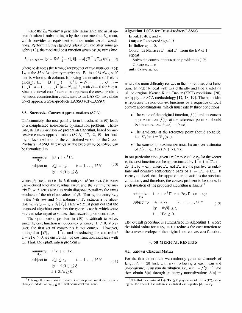
Since the L0 "norm" is generally intractable, the usual approach taken is substituting it by the more tractable L\ norm, which provides an equivalent solution under certain conditions. Performing this standard relaxation, and after some algebra [13], the modified cost function given by (8) turns into
Jt CP-LASSO \y-*P\\l + \\\p\\1+p\\(BT<S>IM)Ph, (9)
where <g> denotes the Kronecker product of two matrices [15]; I M is the M x M identity matrix; and B T is a 2MNmin x N matrix whose n-th column, following the notation of [16], is given by b„ = BT(: , n) = [/3T[n - JVmin], . . . , /3T[n -1], / 3 T [n+ l ] , . . . , /3T [n-JVm i n]]T , with/3 = 0 for*; < 0. Since the novel cost function incorporates the cross-products between reconstruction coefficients to the LASSO, we call the novel approach cross-products LASSO (CP-LASSO).
3.3. Successive Convex Approximations (SCA)
Unfortunately, the new penalty term introduced in (9) leads to a complicated non-convex optimization problem. Therefore, in this subsection we present an algorithm, based on successive convex approximations (SCA) [17, 18, 19], for finding a (local) solution of the constrained version of the Cross-Products LASSO. In particular, the problem to be solved can be formulated as
minimize | | /3 | | i+c Tc
subject to |/?fc| = cfc, k
l | y - * / 3 | | 2 < £ ,
,MN (10)
where (3k (resp. ck) is the A;-th entry of (3 (resp c), £ is some user-defined tolerable residual error, and the symmetric matrix T, with zeros along its main diagonal, penalizes the cross products of the absolute values of /3. That is, the entry ~/k,£ in the A;-th row and ^-th column of I \ induces a penalization "fk/CkCe = lk,APk\\PA- Here we must point out that the proposed algorithm considers the general case in which some 7^/ can take negative values, then rewarding co-ocurrence.
The optimization problem in (10) is difficult to solve, since the cost function is not convex whenever T ^ 0. Moreover, the first set of constraints is not convex. However, noting that ||/3||i = l c , and introducing the constraint2
1 + 2rc > 0, we ensure that the cost function increases with Cfc. Thus, the optimization problem is
Algorithm 1 SCA for Cross-Products LASSO Input: T, <&, £ andy. Output: Recovered signal /3. Initialize Co = 0. Obtain the Matrices T + and F from the EV of T repeat
Solve the convex optimization problem in (12) Update c0 = c
until Convergence
where the main difficulty resides in the non-convex cost function. In order to deal with this difficulty and find a solution of the original Karush-Kuhn-Tucker (KKT) conditions [20], we apply the SCA methodology [17, 18, 19]. The main idea is replacing the non-convex functions by a sequence of local convex approximations, which must satisfy three conditions:
• The value of the original function, /(•), and its convex approximation, /(•), at the reference point x0 should be the same, i.e., / (x 0 ) = / (x 0 ) .
• The gradients at the reference point should coincide, i.e., V / (x 0 ) = V^xo) .
• The convex approximation must be an over-estimator o f / ( - ) , i . e . , / ( x )> / (x ) ,Vx .
In our particular case, given a reference value c0 for the vector c, the cost function can be approximated by l T c + c T T + c + 2C([r_(c - c0), where T + and r _ are the positive semidef-inite and negative semidefinite parts of T = T + + r _ . It is easy to check that this approximation satisfies the previous conditions, and therefore, the convex problem to be solved in each iteration of the proposed algorithm is finally,3
minimize 1 c + c T+c /3,c
subject to |/?fc| < Cfc, k = 1
l | y - * / 3 | | < £ 1 + 2Tc > 0.
2 c T r _ ( c - c 0 )
,MN (12)
The overall procedure is summarized in Algorithm 1, where the initial value for c (c0 = 0), reduces the cost function to the convex envelope of the original non-convex cost function.
4. NUMERICAL RESULTS
minimize 1 c + c Tc
subject to |/?fc|<Cfc, k=l,...,MN Q ^ )
l | y - * / 3 | | 2 < £ l + 2 rc > o,
2Although this constraint is redundant at this point, and it can be completely avoided if all 7fc £ > 0, it will become relevant soon.
4.1. Known Channel Matrix
For the first experiment we randomly generate channels of length L = 20 first, with h[n] following a zero-mean and unit-variance Gaussian distribution, i.e., h[n] ~ 7V(0,1), and then obtain h[n] through an energy normalization: h[n] =
3Note that the constraint 1 + 2 r c > 0 plays a crucial role in (12), ensuring that the first set of constraints is satisfied with equality |/3j. | = ck.
Table 1. Results (averaged over 100 experiments) for unknown channel matrix using a Hanning window as basis element in the reconstruction dictionary when L = Nn 10.
LASSO CP-LASSO -̂ »min K Nr Nd Nfa Nr Nd Nfa
5 10 15 20 25
73.32 42.02 29.54 22.86 18.62
34.41 11.66 5.73 3.33 3.38
34.12 11.65 5.73 3.33 3.38
0.29 0.01 0.00 0.00 0.00
60.79 31.38 19.24 13.33 12.15
52.81 29.31 18.85 13.14 12.11
7.97 2.07 0.39 0.18 0.04
Table 2. Results (averaged over 100 experiments) for random known channel matrices when L = 20 and SNR = 10 dB.
M n ] / \ / r En=o |^M|2- The amplitudes of the arrivals also follow a Gaussian distribution, A& ~ A/"(0,1), and the number of zero samples between two consecutive spikes is equal to Wmin plus a discretized Poisson process with rate K (i.e., the expected inter-arrival time is A^min + {K + 1)/K). The channel matrix is assumed to be known, so we set $ = H.
Table 2 shows the results when K = 1 and N = 500 for LASSO (which corresponds to using (10) with V = 0) and CP-LASSO (p = 100). Since we are interested in recovering the latent spikes, this table shows the number of activations recovered (Nr\ the number of correctly located detections (Nd), and the number of false alarms (Nfa), altogether with the average number of spikes (K). CP-LASSO outperforms LASSO regarding Nd, although at the expense of a higher value of Nfa in this case.
4.2. Unknown Channel Matrix
For the second example we use activations that follow the shape given in [21] for electrograms with L = 11. The amplitude of the activations is again normally distributed, i.e., Ak ~ 7V(0,1), and the negative co-occurrence period is set to Nm[n = 10. The activations arrive periodically now, with a period equal to Nm[n + 1. We assume an unknown channel with a known length, and use a Hanning window of length L = 10 to generate the reconstruction dictionary. Table 1 shows the results for L = 10 in terms of the number of correct detections (Nd (k) is the number of detections within distance k of a true activation, i.e., Nd(0) = Nd in Table 2), number of violations of the negative co-occurrence period (Nv) and number of false alarms (Nfa). In this case CP-LASSO outperforms LASSO w.r.t. all performance measures.
0.12
0.1
0.08
0.06
0.04
0.02
0
•0.02
i "0 20 40 60 80 100
Fig. 1. Activations recovered using LASSO (dashed black line) and CP-LASSO (each colour corresponds to a different basis function).
Finally, we show an example of the activations recovered using an overcomplete dictionary with M = 3 in Figure 1. The synthetic data are generated using a random channel with L = 20, N = 100 and 7Vmin = 10. We build the reconstruction dictionary using the mexican hat wavelet with three different variances: a\ = 0.1, a\ = 1 and a\ = 10. The signal contains 8 activations. Using LASSO we recover 8 activations, not always significant, and we have two violations of the negative co-occurrence period. Using CP-LASSO we only detect 6 activations, but there are no violations of the co-occurrence period and all of them are relevant.
5. DISCUSSION
In this paper we have shown how to incorporate a negative co-occurrence restriction into a sparse learning problem. The proposed approach builds on LASSO, adding a novel penalty term. Although some authors have derived approaches to obtain sparse signals that respect some physical/biological restrictions in the past (see e.g. [7, 8, 9]), no approach based on the cross-products has been developed in the literature as far as we know. Finally, we also make use of the successive convex approximations (SCA) idea in order to optimize the resulting non-convex problem.
6. REFERENCES
[1] Robert M. Haralick, K. Shanmugam, and Its'Hak Din-stein, "Textural features for image classification," Sys-tems, Man and Cybernetics, IEEE Transactions on, vol. SMC-3, no. 6, pp. 610 -621, nov. 1973.
[2] Myung Jin Choi, J.J. Lim, A. Torralba, and A.S. Will-sky, "Exploiting hierarchical context on a large database of object categories," in Computer Vision and Pattern Recognition (CVPR), 2010 IEEE Conference on, June 2010, pp. 129 -136.
[3] J. Jalife, M. Delmar, J. Anumonwo, O. Berenfeld, and J. Kalifa, Basic Cardiac Electrophysiology for the Clinician, Wiley, 2 edition, 2011.
[4] G. F. Knoll, Radiation Detection and Measurement, Wiley, 3nd edition, 2000.
[5] Bruno A. Olshausen and David J. Fieldt, "Sparse coding with an overcomplete basis set: a strategy employed by vl," Vision Research, vol. 37, pp. 3311-3325, 1997.
[6] Julien Mairal, Francis Bach, Jean Ponce, and Guillermo Sapiro, "Online learning for matrix factorization and sparse coding," /. Mack Learn. Res., vol. 11, pp. I9 60, Mar. 2010.
[7] R.G. Baraniuk, V. Cevher, M.F. Duarte, and C. Hegde, "Model-based compressive sensing," IEEE Transactions on Information Theory, vol. 56, no. 4, pp. 1982 -2001, Apr. 2010.
[8] R. Tibshirani, M. Saunders, S. Rosset, J. Zhu, and K. Knight, "Sparsity and smoothness via the fused lasso," Journal of the Royal Statistical Society Series B, vol. 67, no. 1, pp. 91-108, 2005.
[9] H. Zou and T. Hastie, "Regularization and variable selection via the elastic net," Journal of the Royal Statistical Society. Series B, vol. 67, no. 2, pp. 301-320, Jan. 2005.
[10] L. Yu, H. Sun, J. P. Barbot, and G. Zheng, "Bayesian compressive sensing for cluster structured sparse signals," Signal Processing, vol. 92, no. 1, pp. 259-269, Jan. 2012.
[11] YC. Eldar, P. Kuppinger, and H. Bolcskei, "Block-sparse signals: Uncertainty relations and efficient recovery," IEEE Transactions on Signal Processing, vol. 58, no. 6, pp. 3042 -3054, June 2010.
[12] Sandra Monzon, Tom Trigano, David Luengo, and Antonio Artes-Rodriguez, "Sparse spectral analysis of atrial fibrillaion electrograms," in 2012 IEEE Machine Learning for Signal Processing Workshop (MLSP), San-tander (Spain), 23-26 Sep. 2012.
[13] David Luengo, Javier Via, Sandra Monzon, Tom Trigano, and Antonio Artes-Rodriguez, "Blind analysis of EGM signals: Sparsity-aware formulation," Tech. Rep., Die. 2012, arXiv.
[14] R. Tibshirani, "Regression shrinkage and selection via the LASSO," Journal of the Royal Statistical Society, vol. 58, no. 1, pp. 267-288, 1996.
[15] Charles F. Van Loan, "The ubiquitous Kronecker product," Journal of Computational and Applied Mathematics, vol. 123, pp. 85-100, 2000.
[16] Gene H. Golub and Charles F. Van Loan, Matrix Computations, The John Hopkins University Press, Baltimore, MA (USA), 3rd edition, 1996.
[17] M. Chiang, Chee Wei Tan, D.P Palomar, D. O'Neill, and D. Julian, "Power control by geometric programming," IEEE Transactions on Wireless Communications, vol. 6, no. 7, pp. 2640-2651, July 2007.
[18] Barry R. Marks and Gordon P. Wright, "A general inner approximation algorithm for nonconvex mathematical programs," Operations Research, vol. 26, no. 4, pp. 681-683, 1978.
[19] M. Avriel, Advances in geometric programming, Plenum Press, New York, 1980.
[20] Stephen Boyd and Lieven Vandenberghe, Convex Optimization, Cambridge University Press, March 2004.
[21] Gerald Fischer, Markus Ch. Stuhlinger, Claudia-N. Nowak, Leonard Wieser, Bernhard Tilg, and Florian Hintringer, "On computing dominant frequency from bipolar intracardiac electrograms," IEEE Transactions on Biomedical Engineering, vol. 54, no. 1, pp. 165-169, January 2007.