Computational Ecology and Software, 2019, 9(1): 19-36 IAEES www.iaees.org Article Crowding effects and depletion mechanisms for population regulation in prey-predator intraspecific competition model Kumar G. Ranjith 1 , Das Kalyan 2 , K. Lakshminarayan 3 , Reddy B. Ravindra 4 1 Department of Mathematics, Anurag Group of Institutions, Venkatapur, Hyderabad-500 088, India 2 Department of Basic and Applied Sciences, National Institute of Food Technology Entrepreneurship and Management, Kundli, Sonepat, Haryana -131028, India 3 Department of Mathematics, Vidya Jyothi Institute of Technology, Moinabad, Hyderabad-500075, India 4 Department of Mathematics, Jawaharlal Nehru Technological University, Kukatpally, Hyderabad-500085, India E-mail: [email protected], [email protected], [email protected], [email protected]Received 11 October 2018; Accepted 20 November 2018; Published 1 March 2019 Abstract The current investigation centres on the consequences of intra-specific rivalry involving predators in the predator-prey equation. A careful account of the investigation is offered mathematically of the model to offer insights into important outcomes that result from the interplay of deterministic and stochastic process. In particular, the steadiness and bifurcation investigation of this model find mention. Allowance is also made in this model for a stochastic environment impacted by white noise. While for this particular version, the global stability is predicated under conditions bordering on stochasticity close to environmental concerns. Rivalry among the predator population is without a doubt accommodating for a various predator-prey models by keeping population stable at a positive interior equilibrium. Numerical solutions obtained for the models support the assumptions governing the study. Keywords intraspecific competition; Hopf-bifurcation; stochasticity; Lyapunov function; discrete model; white noise. 1 Introduction Mathematical models of population dynamics find expression in terms of difference or differential equations that detail how populations change with time, space or particular stages of development (Zhang, 2015, 2016). Although research in the field of population dynamics, traditionally the preserve of mathematical ecology, can be found in accounts of 18 th century, a watershed of its arrival as a scientific discipline and its subsequent respectability may be attributed to the works of Alfred J.Lokta and Vito Volterra. To begin with, actual instances of individual behaviour accompany the concept of functional response, defined as the rate at which an individual predator consumes prey in terms of density of prey. Plenty of Computational Ecology and Software ISSN 2220721X URL: http://www.iaees.org/publications/journals/ces/onlineversion.asp RSS: http://www.iaees.org/publications/journals/ces/rss.xml Email: [email protected]EditorinChief: WenJun Zhang Publisher: International Academy of Ecology and Environmental Sciences
Transcript
Computational Ecology and Software, 2019, 9(1): 19-36
IAEES www.iaees.org
Article
Crowding effects and depletion mechanisms for population regulation
in prey-predator intraspecific competition model
Kumar G. Ranjith1, Das Kalyan2, K. Lakshminarayan3, Reddy B. Ravindra4 1Department of Mathematics, Anurag Group of Institutions, Venkatapur, Hyderabad-500 088, India 2Department of Basic and Applied Sciences, National Institute of Food Technology Entrepreneurship and Management, Kundli,
Sonepat, Haryana -131028, India 3Department of Mathematics, Vidya Jyothi Institute of Technology, Moinabad, Hyderabad-500075, India 4Department of Mathematics, Jawaharlal Nehru Technological University, Kukatpally, Hyderabad-500085, India
Mathematical models of population dynamics find expression in terms of difference or differential equations
that detail how populations change with time, space or particular stages of development (Zhang, 2015, 2016).
Although research in the field of population dynamics, traditionally the preserve of mathematical ecology, can
be found in accounts of 18thcentury, a watershed of its arrival as a scientific discipline and its subsequent
respectability may be attributed to the works of Alfred J.Lokta and Vito Volterra.
To begin with, actual instances of individual behaviour accompany the concept of functional response,
defined as the rate at which an individual predator consumes prey in terms of density of prey. Plenty of
Computational Ecology and Software ISSN 2220721X URL: http://www.iaees.org/publications/journals/ces/onlineversion.asp RSS: http://www.iaees.org/publications/journals/ces/rss.xml Email: [email protected] EditorinChief: WenJun Zhang Publisher: International Academy of Ecology and Environmental Sciences
Computational Ecology and Software, 2019, 9(1): 19-36
IAEES www.iaees.org
literature is available that has already discussed ecological systems (Arditi et al., 1989; Freedman et al., 1980;
Gatto et al., 1991; May et al., 1973), where the model systems are based on prey-dependent model systems. In
all the cases the functional response which is prey-dependent is modelled as
22 2 2, ,ax x ax x ax x x or some equivalent form. The Holling-Tanner model deals
with the Michaelis-Menten or Holling type –II functional response of the form cx m x . Where c is the
maximal predator, per capita utilization rate, i.e., the most extreme number of prey that can be devoured by a
predator in each time unit and m is the half catching immersion consistent i.e., the quantity of prey important
to accomplish one-half portion of the greatest rate c. Such functional responses go by the name of “prey-
dependent”, named as such by Arditi and Ginzburg, in view of the fact that it depends on prey density only. It
was realised early on that the predator density could directly impact functional response. Plenty of such
predator-dependent models (Akcakaya et al., 1995; Cosner et al., 1999; Gutierrez et al., 1992; Hanski et al.,
1991; Arditi et al., 1992; Gutirrez et al., 1992; Blaine et al., 1997; Poggiale et al., 1998; Cosner et al., 1999]
have been in the offing, the most well - known being Hassell and Varley, 1969; Detngeles et al., 1975. Arditi
and Ginzburg 1989, 1991; presented a Michaelis-Menten type ratio dependent functional response of the form
cx my x , where x, y stand for densities of prey and predator respectively.
This article intends to propose a model with intraspecific competition between predators with half
saturation constant, before this so many authors investigated prey-predator models with intraspecific
competition without saturation constant. Intraspecific competition among predators for prey starts the minute
the ratio of predators to prey is sufficiently large, leading to individuals among the predator population
undergoing reduced fitness from absence of sustenance (Purves et al., 2001). This extreme competition
happens in blue crab populations where they express brutal behaviour, leading to bloodied wounds due to
scarcity (Clark et al., 1999). More extreme intra specific competition has been known to happen in intra
specific predation in a variety of predator populations due to limited availability of alternative food source
(Fox, 1975). Finally, it is surmised that competition within the predator population might be advantageous for
predator species under specified circumstances in deterministic environment.
However, the deterministic environment rarely occurs in reality since most natural environments display
randomness. Most of what shows up in the models proposed and explored in the ecological literature operate is
in the framework of an unchanging, deterministic ambience. That is, real environments tend to be uncertain
and stochastic.
Frankly, randomness or stochasticity majorly impacts the structure and function of biological systems
(May, 1974; Renshaw, 1995; Nisbet and Gurney, 1982; Samanta, 1996). The environmental factors are usually
time-dependent, randomly changing and are to be treated as stochastic. Renshaw (1995) maintain that natural
phenomena of whatever persuasion defy purely deterministic laws and toggle randomly around some average,
so much so as to enable the deterministic equilibrium to suffer the loss of an absolutely fixed state; instead it
pans out towards a “fuzzy” value, surrounding the biological system it is concerned with. A primary hurdle in
the stochastic modelling of an ecosystem is the lack of reliable mathematical wherewithal at hand to analyze
Samanta and Maiti, 2003, 2004; Bandyopadhyay and Chakrabarti, 2003; Bandyopadhyay and Chattopadhyay,
2005; Maiti and Samanta, 2005, 2006; Maiti et al., 2007) found out the comparison between deterministic and
stochastic models with good accuracy.
We also considered discrete version of the considered continuous population model. Generally, discrete
20
Computational Ecology and Software, 2019, 9(1): 19-36
IAEES www.iaees.org
model shows richer dynamics than continuous models. Based on this many researchers (Liu et al., 2007;
Lopez-Ruiz et al., 2004; Elsadany et al., 2012) have considered these models to discuss the population
dynamics of prey- predator models. Usually discrete models are described with difference equations. Also, we
can easily obtain numerical simulations for discrete models.
This paper is organized as follows: Section 3 discusses the boundedness of the system; Section 4
permanence of the system, Section 5 throws equilibrium points, existence, and stability and bifurcation
analysis of the model. Section 6 defined discrete version of the mathematical models, Section 7 and 8 throws
equilibrium points, their stability and bifurcation analysis, Section 9 throws light on stochastic stability of the
system by using Lyapunov function. Section 10 explores numerical simulation of the system which supports
analytical results arrived at.
2 Formulation of Deterministic Mathematical Model
In this section we have constructed a mathematical model of Prey-predator with intraspecific competition
between predators. The model can be presented by the following set of ordinary differential equations
2
1
dx x xyrx
dt k x
dy e xy ydy
dt x L y
(2.1)
with initial conditions 0 0, 0 0x y , where x(t), y(t) represents prey and predator population biomass,
r stands for intrinsic growth rate of prey, k carrying capacity, conversion rate , saturation constant, e
another conversion rate, d represents death coefficient of predator, rate of predator inter competition, L
saturation constant. All the model parameters are positive constants.
This model involves certain assumptions which consist of the followings:
(i) Prey individuals are assumed to have the logistic growth rate with carrying capacity K.
(ii) The Prey- dependent functional response is assumed in the interaction between prey and
predator Population.
(iii) We assumed intraspecific competition among the predators.
3 Behaviour of the Solutions of Deterministic Model
Theorem 1. The solutions of the system (1) are invariant under 2R .
Proof: we can easily verify that 1 20,0 0,0 0F F , then from this we can say that 1 ,F x y and
2 ,F x y are continuous on 2R and also Lipschizian on 2R . Hence solution of (1) exists and it is unique.
These solutions are exist for all 0t and stay non-negative. Hence, the interior of 2R is invariant under
model system (1).
Theorem 2. The solutions of the system (1) are bounded.
Proof: Let W x y
21
Computational Ecology and Software, 2019, 9(1): 19-36
IAEES www.iaees.org
dW dx dy
dt dt dt
(3.1)
( 1) min 1,dW
x r mW where m ddt
and also 1dx x
rxdt K
then by a standard comparison
theorem we have lim ( ) (0),t
Supx t M where M x K
.
Therefore ( 1)dW
mW M rdt
(3.2)
Applying the theorem in differential inequalities (Birkhoff et al., 1962), we obtain
10 , (0), (0) / mtM r
W x y W x y em
and for
1,0
M rt W
m
.
Therefore all solutions of system (2.1) enter into the region
2 1, : , 0
M rB x y R W for any
m
.
(3.3)
4 Permanency of the System
Theorem 3. If ( , ) 0 x y then the solution of the system (2.1) is permanent.
Proof: Consider the Lyapunov function 1 2( , ) p ph x y x y , where 1 2,p p are positive constants.
In positive octant.
1 1 2 2( , ) / / / x y h h p F x p F y . To show the system has permanence of the solution
we required to show ( , ) 0 x y at axial equilibrium point (E2). Here it is clearly exist without any condition.
Hence the system has a permanent solution with unconditionally.
5 Existences of the Equilibrium Points and Their Stability Analysis
In this section we will study the existence and stability behaviour of the system (2.1) at various equilibrium
points. The equilibrium points of the system (2.1) are
(i) Trivial equilibrium : 1(0,0)E
22
Computational Ecology and Software, 2019, 9(1): 19-36
IAEES www.iaees.org
(ii) Persistent equilibrium : 2 ( ,0)E k
(iii) Interior equilibrium : 3 2 2( , )E x y
where 2
22 2( ) ( )
dL d yx
L y e dL d y and 2y is the root of the following equation.
3 21 2 3 4 0 y y y (5.1)
where
21
2 2 22
2 2 2 2 2 2 2 23
2 2 2 2 2 24
( ) ;
( ) 2 ( )( );
( ) (2 1) ;
;
e d
e rk d e r e rk L e d e d
L e d e rd L e Lr e rdkL e rkL e Lrkd e Lrk
L e rd e Lrk e L rkd e L rk
The first two equilibrium points always exist and (5.1) has one and only positive root if 2 34 0 , if
2 34 0 then (5.1) has two equal roots and if 2 34 0 then it has three distinct real roots, where
2 3 21 4 1 2 3 2 1 3 23 2 , . By Cardan’s method, the roots of the equation (5.1) is
21
1( )
AA
, where A denotes the value of 1
32 31
42
. We obtain the remaining roots
of the equation (5.1) by Cardan’s method in a similar manner. Now, for positive root of 2y , one positive
interior equilibrium point is attained provided that 2 2( ) ( ) 0 L y e dL d y .
5.1 Stability and bifurcation analysis of each fixed point
The stability analysis of each equilibrium point finds discussion along with bifurcation analysis of the system
(2.1). In this process, the following notations have been employed.
1 2( , ) ( , ), ( , ) , where ( , )
T TX F X m F x y F x y X x y , and the Jacobian matrix of the system
( , )J AF X m .
5.1.1 Stability analysis at E0
The Jacobian at this equilibrium point is denoted by J0, and is defined as 0
0
0
rJ
d
The Latent values are r,-d. Hence the system (2.1) at equilibrium point E0 is unstable.
5.1.2 Stability analysis at E1
23
Computational Ecology and Software, 2019, 9(1): 19-36
IAEES www.iaees.org
The Jacobian matrix of the system (2.1) at equilibrium point E1 is denoted by J1 and is defined as
The Latent values are ,
e k
r dk
. Therefore the system (2.1) is stable if where( )
d k
ek.
If then one Eigen value of 1J is zero and the other eigen value isr . Let the Eigen vectors of 1J
and 1TJ corresponding to the Latent value ‘0’ are M and N respectively. M and N are defined as
2
2
( )
M
M
kM
r k and 2
2
0
NN
respectively. Here 2 2,M N are two non zero real numbers. Now
, 0 TN F X , where 1 ,0X k . Hence by Sotomayor theorem (Sotomayor, 1973) the system
does not attain any saddle-node bifurcation around E1. Again 2 21, 0
T ekM NN AF X M
k and
21, , 0
TN A F X M M , where
,
AFFF AF . Therefore, by the same theorem
[25] the system experiences a transcritical bifurcation at around the axial equilibrium E1.
5.1.3 Stability analysis at E2
The Jacobian matrix of the system around the equilibrium point E2 (x2, y2) is defined as
2 2 2 22
22
22 2
2 2
2 2
rx x y x
k xxJ
e y Ly
x L y
In above matrix
2 2 2 211
2 2
/0,if <
/ 1 1 /
srx y rx y
ak x x k
2 2 2
12 21 222 22 2 2
0, 0& 0
x e y Lya a a
x x L y
11 22 2 11 22 12 22 10&det( )( ) 0 if < str J a a J a a a a Where 2
2
s r x
ky
1
0
kr
kJe k
dk
24
Computational Ecology and Software, 2019, 9(1): 19-36
IAEES www.iaees.org
Therefore, the system (2.1) is locally asymptotically stable at positive equilibrium point 2 2 2( , )E x y if < s .
5.1.4 Bifurcation analysis
i) Saddle-node bifurcation: To account for the saddle node bifurcation we have to consider 2det( ) 0J
which gives SN and one eigen value of 2J will be zero. Here SN is the solution of the equation
2 2 3 2 3( ) ( ) ( )( ) ( ) ( )k exy L y k xy x k xy x L y r xy x L y .
Let 1 2and be the eigen vectors of 2J and 2TJ corresponding to the eigen value zero. The first eigen
vector 1 is defined as 1 2
Tz and z and 2 1 2,
Th h , where
12 22 21 221 2 2 1 2 2
11 21 11 12
,a a a a
z z z h h ha a a a
, and 2 2,z h are any two non-zero real numbers.
By simple calculation we can verify easily that 2 2 , 0T SNF X and
22 2 1 1, ( , ) 0T SNA F X . Therefore, by Sotomayor theorem [25] the system has saddle -node
bifurcation at positive equilibrium 2 2 2( , )E x y and also the system has neither transcritical nor any pitch-fork
bifurcation at 2 2 2( , )E x y since 2 2 , 0T SNF X .
ii) Hopf-bifurcation: If 2( ) 0tr J which gives HB
where
2 2
2HB rx L y Ly x
xyk L y
and
2 2 3 22 3 2
3
1det( ) [ ( ) ( ) ( )( )
( ) ( )
( ) ( )]
J k exy L y k xy x k xy x L yk x L y
r xy x L y
If 2 2( ) 0&det( ) 0tr J J then the Latent values of 2J will be purely imaginary and by implicit function
theorem, the system undergoes Hopf bifurcation at positive equilibrium 2E .
6 Formulation of the Discrete Mathematical Model
In this section we study the dynamics of discrete predator-prey model with intraspecific competition between
predators, which has the following difference equations
25
Computational Ecology and Software, 2019, 9(1): 19-36
IAEES www.iaees.org
n
nn
n
nnnn
n
nnnnnn
yL
ydy
x
yxyy
x
yx
k
xrxxx
2
1
1 1
(6.1)
where x and y are the population biomasses of the predator and prey generations n and n+1 respectively. In
system (6.1), all the parameters are same as in system (2.1). The map given by equation (6.1) is a noninvertible
map of the plane. The study of the dynamical properties of the above map allows us to have information
about long-run behaviour of the predator–prey populations. Starting from the initial condition 00 , yx , the
interaction of (6.1) uniquely determines a trajectory of the states of population output in the following form:
00 ,, yxTnynx n where ,.........2,1,0n
7 Fixed Points and Stability Analysis
The system (6.1) has two fixed points 1 2E and E and these are exactly same as the fixed points of continuous
model (2.1). Next we have to study the stability of these fixed points.
To discuss the local stability of each fixed point, first we have to compute Jacobian matrix of the system
(6.1) at each fixed point.
2
2 2
1
1
rx xy x
K xxJ
e y Ly
x L y
To study the stability of the fixed points of the system (6.1) we recall the following lemma.
Lemma 1. Let 21 2L L and 1 0
Let 1 2, are two roots of 0 . Then:
i). 1 1 and 2 1 if and only if 1 0 and 0 1
ii). 1 1 and 2 1 if and only if 1 0
iii). 1 1 and 2 1 if and only if 1 0 and 0 1
iv). 1 1 and 2 1 if and only if 1 0 and 1 0,2;L
v). 1 2, are complex and 1 21, 1 if and only if 21 24 0L L and 0 1
A fixed point * *,x y is called a sink if 1 1 and 2 1 , so it is locally asymptotically stable. * *,x y
26
Computational Ecology and Software, 2019, 9(1): 19-36
IAEES www.iaees.org
is called a source if 1 1 and 2 1 , so it is locally unstable. If * *,x y is called a saddle if 1 1 and
2 1 and * *,x y is called a non-hyperbolic if 1 21, 1 .
Theorem 4. Suppose that the fixed point 1E
i).is a sink if 0r and
ii).is a source if 0r and
iii).is a saddle if 0r and
iv).is non-hyperbolic if 1r and where d K
eK
.
Proof: To prove all these results first we have to compute the variation matrix of the system (6.1) at 1E is
1
1
0 1E
Kr
KJe K
dK
The eigen values of above Jacobian matrix are 1 21 , 1e K
r dK
.
By using Lemma1 we can easily verify that 1E is a sink if 1 . ., 0r i e r and
1 1 . .,
d Ke Kd i e
K eK
; 1E is a source if 0r and ; 1E is a saddle if 0r
and and is non-hyperbolic 1r and .
8 Local Stability and Hopf-bifurcation around Interior Point
We now investigate the local stability of positive equilibrium * *,x y . The variation matrix at the positive
equilibrium * *,x y is
2
* **
*1
1E
rx xMx
J K xe M LN
where
* *
2 2* *,
y yM N
x L y
The characterstic equation of this Jacobian matrix is 2 0B C
27
Computational Ecology and Software, 2019, 9(1): 19-36
IAEES www.iaees.org
Where * * * *
* * **
2 , 1rx rx rx e M x
B Mx LN C Mx LN LN LMNxK K K x
Theorem 5: If * * * *
* * **
22 2 3
rx rx e M x rxLMNx LN Mx LN LMNx LN
K K x K
then the
fixed point 2E is locally asymptotically stable.
Proof: In order to prove 2E is locally stable by using Lemma1 we have to verify
1 0, 1 0 1and C .
* *
**
1rx e M x
LN LMNxK x
If * *
**
rx e M xLN LMNx
K x
then 1 0
* * *
* **
21 3 2 2
rx rx e M xMx LN LN LMNx
K K x
If * * *
* **
22 3
rx e M x rxMx LN LN LMNx
K x K
then 1 0
* * ** *
*1 0
rx rx e M xC Mx LN LN LMNx
K K x
Which is true if * * *
* **
rx rx e M xLN LMNx Mx LN
K K x
From above results 2E is locally asymptotically stable if () is exist.
Corollary 1: The fixed point 2E is unstable if and only if the following conditions holds
* * ** *
*
rx rx e M xLMNx LN Mx LN
K K x
, or
* * ** *
*
22 2 3
rx e M x rxMx LN LMNx LN
K x K
.
Corollary 2: Suppose that * * *
* **
22 2 3
rx e M x rxMx LN LMNx LN
K x K
then the system (6.1)
undergoes a Hopf-bifurcation when passes through a critical value c where det 1 cj at .
28
Computational Ecology and Software, 2019, 9(1): 19-36
IAEES www.iaees.org
9 Stochastic Stability of The Deterministic System at Positive Equilibrium Point
To investigate the environmental fluctuations on model (2.1), it is understood that the stochastic perturbations
are of white noise type and that they are proportional to the distances of ( )x t and ( )y t respectively. So
system (2.1) results
11 2
22 2
2
1 t
t
dx x xyrx
dt k x
d
x x d
y y dy e xy y
dydt x L y
(9.1)
where 1 2, are real constants, , 1, 2it i t i are independent of each other standard Wiener
processes. The system (9.1) has the same equilibrium as the system (2.1).
The stochastic differential system (9.1) may then centred at its positive equilibrium 2E by the change of
variables
1 2 2 2,u x x u y y (9.2)
The linearized Stochastic Differential Equations around 2E take the form
du t f u t dt g u t d t (9.3)
where 1 2,T
u t u t u t , 2f u t J , which defined in section (5.1.3) and
1 1 2 2( ) ( , )g u t diag u u .
Let 1,2 20, ,
C be the family of nonnegative functions. ,W t u defined on
20, is a continuously differentiable function with respect to t and twice with respect to u .
We define the differential operator L for a function ,W t u by
2
2
, , ,1( , )
2T TW t u W t u W t u
LW t u f u Tr g u g ut u u
(9.4)
1 2 3
, ,W W W W
colu u u u
, 2 2
2
,, 1, 2
j i
W t u Wi j
u u u
and ‘T ’ means transposition.
With reference to the book by Afanas’ev et al. 1996; the following theorem holds.
Theorem 6. Suppose there exist a function 1,2 2( , ) 0, ,
W t u C satisfying the following
29
Computational Ecology and Software, 2019, 9(1): 19-36
IAEES www.iaees.org
inequalities
1 2,p p
K u W t u K u ; 3, ,p
LW t u K u (9.5)
where 1 2 3, ,K K K and p are positive constants.
Then the trivial solution of (9.3) is exponentially p - stable for 0t Moreover, if in (9.5), 2p the
trivial solution of (9.3) is globally asymptotically stable in probability.
Theorem 7. Suppose that
2 2 2 22
2 21 2 2
2 2
2 , 2rx x y Ly
k x L y
hold. Then, the trivial solution
of (9.3) is asymptotically mean square stable.
Proof: Let us consider the Lyapunov function
2 21 1 2 2
1
2W u w u w u (9.6)
where 1 2,w w are nonnegative constants to be chosen in the following . It is easy to check that inequalities
(9.5) hold true with 2p .
2 2 2 2 2 22 2 2
22
1 1 2 1 2 1 2 2
2
2
2 2
,1
2T
LW u w u u u w u u u
W t uT
rx x y x e y Ly
k xx x L
uu
y
r g u g
(9.7)
with 2
2 2 2 21 1 1 2 2 22
,1 1
2 2T W t u
Tr g u g u w u w uu
If in (9.7) we choose 1
2 222
2 2
x e y
xw w
x
, then
2 2 2 22 2
2 2
2 2 2 21 1 1 2 2 2
1 1
2 2LW u w
rx x y Ly
k x L yu w u
According to Theorem (1), we conclude that the trivial solution of system (9.3) is globally asymptotically
stable.
10 Numerical and Computer Simulation
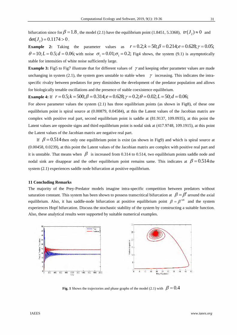
Example1. For the fixed parameter values 0.8, 50, 0.628, 10, 5, 0.06, 0.225r k e L d and varying values, the system moves from stable to unstable or unstable to stable. If varies from 0.4 to
0.66 the system is stable, from 0.67 to 1.8 the system is unstable and the system is stable when greater than 1.8
(Illustrated in Fig. 1, Fig. 2 & Fig. 3). Also, we observed when 1.8HB the system will go under Hopf
30
Computational Ecology and Software, 2019, 9(1): 19-36
IAEES www.iaees.org
bifurcation since for 1.8 , the model (2.1) have the equilibrium point (1.8451, 5.3368), 2( ) 0tr J and
2 0.det 11 4( 0) 7J .
Example 2: Taking the parameter values as 0.2140.2; 50; 0.628; 0.; 05;r k e
10; 0.5; 0.06;L d with noise 1 10.01; 0.2; Fig4 shows, the system (9.1) is asymptotically
stable for intensities of white noise sufficiently large.
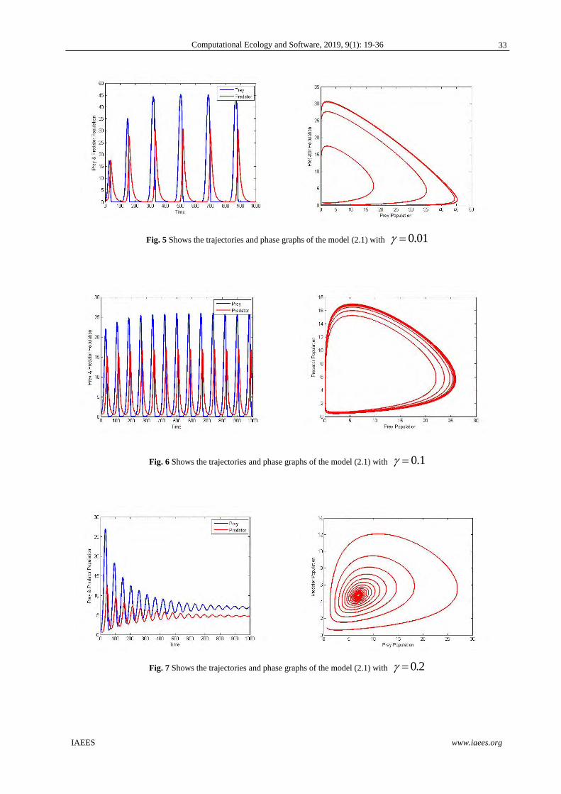
Example 3: Fig5 to Fig7 illustrate that for different values of and keeping other parameter values are made
unchanging in system (2.1), the system goes unstable to stable when increasing. This indicates the intra-
specific rivalry between predators for prey diminishes the development of the predator population and allows
for biologically tenable oscillations and the presence of stable coexistence equilibrium.
Example 4: If 0.5; 500; 0.628; 0.2; 0.02; 50; 0.06;0.314;r k e L d
For above parameter values the system (2.1) has three equilibrium points (as shown in Fig8), of these one
equilibrium point is spiral source at (0.00879, 0.04584), at this the Latent values of the Jacobian matrix are
complex with positive real part, second equilibrium point is saddle at (81.9137, 109.0935), at this point the
Latent values are opposite signs and third equilibrium point is nodal sink at (417.9748, 109.1915), at this point
the Latent values of the Jacobian matrix are negative real part.
If 0.514 then only one equilibrium point is exist (as shown in Fig9) and which is spiral source at
(0.00458, 0.0239), at this point the Latent values of the Jacobian matrix are complex with positive real part and
it is unstable. That means when is increased from 0.314 to 0.514, two equilibrium points saddle node and
nodal sink are disappear and the other equilibrium point remains same. This indicates at 0.514 the
system (2.1) experiences saddle node bifurcation at positive equilibrium.
11 Concluding Remarks
The majority of the Prey-Predator models imagine intra-specific competition between predators without
saturation constant. This system has been shown to possess transcritical bifurcation at around the axial
equilibrium. Also, it has saddle-node bifurcation at positive equilibrium point SN and the system
experiences Hopf bifurcation. Discuss the stochastic stability of the system by constructing a suitable function.
Also, these analytical results were supported by suitable numerical examples.
Fig. 1 Shows the trajectories and phase graphs of the model (2.1) with 0.4
31
Computational Ecology and Software, 2019, 9(1): 19-36
IAEES www.iaees.org
Fig. 2 Shows the trajectories and phase graphs of the model (2.1) with 0.67
Fig. 3 Shows the trajectories and phase graphs of the model (2.1) with 1.8
Fig. 4 Shows the trajectories of the model (9.1) with noise.
32
Computational Ecology and Software, 2019, 9(1): 19-36
IAEES www.iaees.org
Fig. 5 Shows the trajectories and phase graphs of the model (2.1) with 0.01
Fig. 6 Shows the trajectories and phase graphs of the model (2.1) with 0.1
Fig. 7 Shows the trajectories and phase graphs of the model (2.1) with 0.2
33
Computational Ecology and Software, 2019, 9(1): 19-36
IAEES www.iaees.org
0 100 200 300 400 500
0
100
200
300
400
500
x
y
Fig. 8 Illustrates the three equilibrium points of the system (2.1)
Fig. 9 The equilibrium point 3E
References
Afanasev VN, Kolmanowski VB, Nosov VR. 1996. Mathematical Theory of Control System Design. Kluwer
Academic, Dordrecht, Netherlands
Akcakaya H, Arditi R, Ginzburg L. 1995. Ratio-dependent predation: an abstraction that works. Ecology,
76(3): 995
Arditi R, Ginzburg LR, 1989. Coupling in predator-prey dynamics: ratio-dependence. Journal of Theoretical
Biology, 139: 311-326
Arditi R, Ginzburg LR, Akcakaya HR. 1991. Variation in plankton densities among lakes:a case for ratio-
dependent models. American Naturalist, 138: 1287-1296
Arditi R, Saiah H. 1992. Empirical evidence of the role of heterogeneity in ratio-dependent consumption,
Ecology, 73: 1544-1551
Bandyopadhyay M, Chakrabarti CG. 2003. Deterministic and stochastic analysis of a non-linear prey-predator
system. Journal of Biological Systems, 11: 161-172
Bandyopadhyay M, Chattopadhyay J. 2005. Ratio-dependent predator-prey model: effect of environmental
0 100 200 300 400 500
0
100
200
300
400
500
x
y
34
Computational Ecology and Software, 2019, 9(1): 19-36
IAEES www.iaees.org
fluctuation and stability. Nonlinearity, 18: 913-936
Birkhoff G, Rota GC. 1962. Ordinary Differential Equations. Ginn Boston, USA
Blaine TW, DeAngelis DL. 1997. The effects of spatial scale on predator-prey functional response. Ecological
Modelling, 95: 319-328
Clark ME,Wolcott TG, Wolcott DL, Hines AH. 1999. Intraspecific interference among foraging blue crabs
Callinectes sapidus: Interactive effects of predator density and prey patch distribution. Marine Ecology
Progress Series, 178: 69-78
Cosner C, DeAngelis DL, Ault JS, Olson DB. 1999. Effects of spatial grouping on the functional response of
predators. Theoretical Population Biology, 56: 65-75
DeAngelis DL, Goldstein RA, O’Neill RV. 1975. A model for trophic interaction. Ecology, 56: 881-892
Dimentberg MF. 1988. Statistical Dynamics of Non-linear and Time-varying Systems. John Wiley and Sons,
New York, USA
Dimentberg MF. 2002. Lotka-Volterra system in a random environment. Physics Review E, 65(3): 036204-1–
6
Elsadany Abd-Elalim A, El-Metawally HA, Elabbasy EM, Agiza HN, 2012. Chaos and bifurcation of a