* OTIC FILE COPY

Winter Environment of theOhio River ValleySteven F. Daly, Michael A. Bilello and Roy E. Bates December 1990

cl)

-a

ain a o w

ha

CRREL Report 90-12

U.S. Army Corpsof EngineersCold Regions Research &Engineering Laboratory

Winter Environment of theOhio River ValleySteven F. Daly, Michael A. Blello and Roy E. Bates December 1990

Acsion ForINTIS CRAWIDTIC lTAB 0

~Ua ;;o!Acd 0J .t ikCdtiof

D i. t lb -tio,- -----------1 1+ "b'jify Codes

Prepared for

OFFICE OF THE CHIEF OF ENGINEERS

ApProved for public release; distribution Is unlimited.

PREFACE

This report was prepared by Steven F. Daly, Research Hydraulic Engineer, Ice Engineering Re-search Branch, U.S. Army Cold Regions Research and Engineering Laboratory, Michael A. Bilello,Meteorologist, Science and Technology Corporation, Hampton, Virginia, and Roy E. Bates, Meteor-ologist, Geophysical Sciences Branch, U.S. Army Cold Regions Research and Engineering Labora-tory.

This report was funded by the Office of the Chief of Engineers, Directorate of Civil Works, underthe River Ice Management Program, Work Unit CWIS 32227, Forecasting Ice Conditions on InlandWaterways. Larry Gatto and Kevin Carey of CRREL provided technical revicws of this report.

The authors thank Guenther Frankenstein, Chief, Ice Engineering Research Branch, for his supportduring this project; Joyce Putnam, mathematics aid with the CRREL Geophysical Sciences Branch,for extracting and tabulating climatic dataduring the initial phase of the study; the computer specialistsof the Engineering and Measurement Services Branch at CRREL for their programming; PamelaBosworth of the CRREL Word Processing Center for her contribution; and the CRREL TechnicalCommunication Branch for drafting the figures and preparing the report for publication. The U.S. AirForce Environmental Technical Application Center's section located at the National Climatic Center,Asheville, North Carolina, also merits special recognition and thanks for providing CRREL thenecessary NOAA publications.

The contents of this report are not to be used for advertising or promotional purposes. The citationof brand names does not constitute an official endorsement or approval of the use of such commercialproducts.

CONTENTSPage

Preface ........................................................................................................................................ iiMetric conversion factors ........................................................................................................... vIntroduction ................................................................................................................................ 1Physical setting and hydrology .................................................................................................. 1

Geographic setting ................................................................................................................ IPhysiographic setting .......................................................................................................... 5Hydrology .............................................................................................................................. 5River ice ................................................................................................................................ 9

Winter climate ............................................................................................................................ 22Air temperature regime for November through March ....................................................... 22Precipitation regime for November through March ........................................................... 23

Conclusions ................................................................................................................................ 32Literature cited ........................................................................................................................... 43Appendix A: Daily air temperatures, water temperatures and discharges at two locations on

the Ohio River ....................................................................................................................... 45

ILLUSTRATIONS

Figure1. Ohio River and its tributaries ............................................................................................ 22. Average annual total precipitation .................................................................................... 43. Location of U.S. Geological Survey river gauging stations ............................................... 64. Long-term average discharges for various basin drainage areas ....................................... 75. Average monthly discharges ............................................................................................. 86. Location of the Ohio River Valley Water SanitationCommission water temperature sites 107. Long-term water temperatures along the Ohio River ....................................................... 118. Annual distribution of mean daily minimum, average and maximum water temperatures

at the Ohio River Valley Water Sanitation Commission water temperature sites ..... 119. Periods when ice was observed on the Ohio River at Cincinnati during each winter ........ 19

10. Total number of days when ice was observed on the Ohio River at Cincinnati duringeach winter ............................................................................................................. 20

11. Total seasonal freezing degree-days at Cincinnati during each winter ............................ 2012. Ratio of total number of days of ice on the Ohio River divided by the total seasonal

freezing degree-days for each winter ...................................................................... 2113. Relationship between ratio values and population trends at Cincinnati, Ohio, since 1900.. 2114. Climatic station number and location map for station names ......................................... 2415. Average air temperatures ................................................................................................. 2616. Approximate topographic contour map .......................................................................... 3117. Relationship between station elevation and average January air temperature ................. 3218. Mean minimum air temperatures .................................................................................... 3319. Total seasonal mean freezing degree-days ..................................................................... 3820. Total water-equivalent precipitation ............................................................................... 3921. Relationship between average January air temperature and total 5-month water equiva-

lent precipitation ...................................................................................................... 4122. Average total annual and maximum monthly snowfall amounts .................................... 42

iii

TABLES

Table Page1. U.S. Army Corps of Engineers lock and dam sites on the Ohio River ............................. 32. U.S. Geological Survey gauging stations along the Ohio River ....................................... 53. Mean daily average water temperatures on the Ohio River, and amplitude and phase

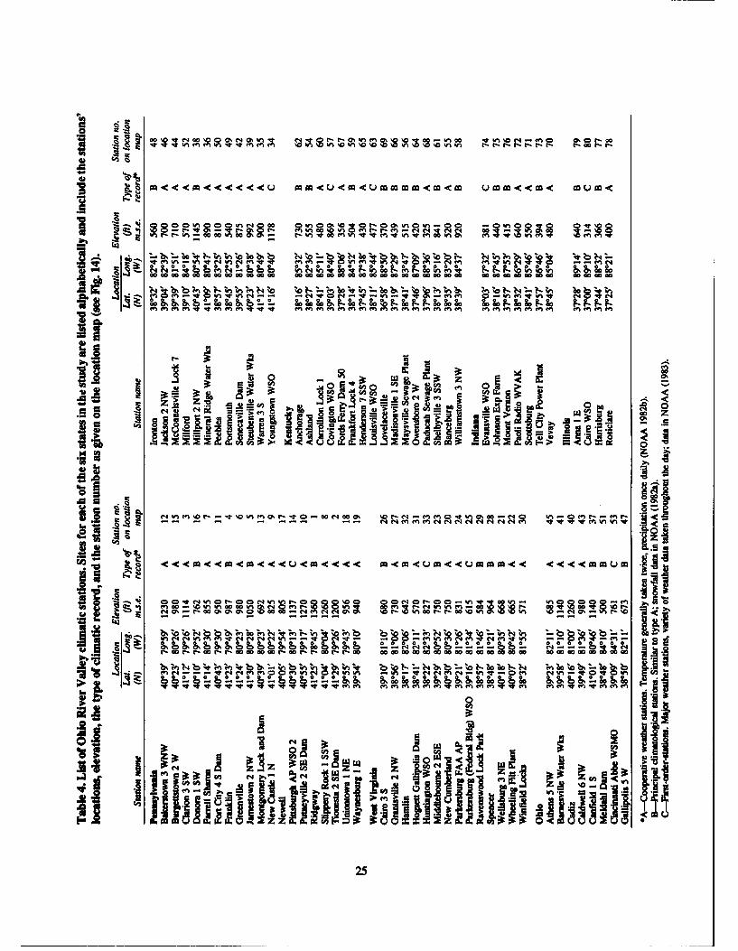
angle values ............................................................................................................. 94. List of Ohio River Valley climatic stations .................................................................. 255. Station summaries of total mean freezing degree-days for the winter season, total water-

equivalent precipitation for the 5-month period November through March, andmean annual and maximum monthly snowfall amounts for type B stations only ..... 40

iv

CONVERSION FACTORS: U.S. CUSTOMARY TO METRIC(SD) UNITS OF MEASUREMENT

These conversion factors include all the significant digits given inthe conversion tables in the ASTM Metric Practice Guide (E 380),which has been approved for use by the Department of Defense.Converted values should be rounded to have the same precision asthe original (see E 380).

Multiply By To obtain

inch 25.4 millimeterfoot 0.3048 metermile (U.S. statute) 1609.347 metermile2 (U.S. statute) 2589669.0 meter2

foot3/second 0.02831685 meter3/seconddegrees Fahrenheit tc = (tF - 32)/1.8 degrees Celsius

V

Winter Environment of the Ohio River Valley

STEVEN F. DALY, MICHAEL A. BILELLO AND ROY E. BATES

INTRODUCTION empties into the Mississippi River (Fig. 1). Except forthe first 40-mile section, which lies entirely in Pennsyl-

One of the major objectives of the River Ice Man- vania, the Ohio River serves as the state boundary be-agement (RIM) Program was to develop a method of tween Ohio, Indiana and Illinois on the north, and Westforecasting river ice conditions that can be used as a Virginia and Kentucky on the south. Major tributariesnavigation aid. The initial focus of the RIM program include the Beaver River in Pennsylvania; the Musk-was on the Ohio River, where ice has severely impeded ingum, Scioto and Great Miami rivers in Ohio; thenavigation in the past. The formation of ice on any river Kanawha River in West Virginia; the Big Sandy Riveris governed by the geographic, hydrologic, hydraulic in West Virginia and Kentucky; the Licking, Green,and climatic conditions of a region. These conditions Cumberland and Tennessee rivers in Kentucky; and thecontrol the heat transfer from river water to the atmo- Wabash River in Indiana and Illinois.sphere, which in turn determines the water temperature Major population centers along the Ohio includeand ultimately controls the formation of ice. In addition, Pittsburgh, Pennsylvania; Wheeling, Parkersburg andsince these conditions can very along a river, the distri- Huntington, West Virginia; Covington-Newpoit andbution of ice along it can vary. Louisville, Kentucky; Portsmouth andCincinnati, Ohio;

As a first step in developing an ice forecast method- and Evansville, Indiana. The river is the primary sourceology for the Ohio River, we compiled data on the of potable water for over three million people, servingphysical setting, hydrology, river ice conditions and the needs of51 private and public water supply utilities.climatology for its region. This report provides a gener- Over 100 industries also take water from the river foral survey of these data--describing the physical setting process use, including cooling water for power plants.and hydrology of the Ohio River Valley and reviewing Hydropower facilities are either in place or planned atpast ice conditions observed on the river-and analyzes each of the 20 Corps of Engineers navigational lock-the winter climate for the region. The report is also and-dam projects along the river.intended to increase our understanding of ice processes The Ohio River is considered a vital link in the inlandon the Ohio River, and to provide information useful for navigation system ofthe United States. Majorcommod-further studies. ities transported include coal, refined and crude oil,

chemicals, fertilizers, steel and grain. Approximately170 million tons of goods were transported on the river

PHYSICAL SETlING AND HYDROLOGY in 1979 (U.S. Army Corps of Engineers 1981).The Corps of Engineers operates 20 locks and dams

Geographic setting on the Ohio River (Table 1), which allow navigation onThe Ohio River is 981 miles long and drains an area the river to proceed throughout the year. A navigation

of approximately 203,900 mi2 , including parts of New channel of 9-ft depth is maintained on the Ohio and onYork, Pennsylvania, West Virginia, Ohio, Indiana, severaltributaries, including the Allegheny, Mononga-Kentucky, Illinois, Tennessee, Mississippi, Alabama, hela, Kanawha, Kentucky, Green, Cumberland andGeorgia, North Carolina, Virginia and Maryland. The Tennessee rivers.river begins at Pittsburgh, Pennsylvania, at the conflu- The lock and dam system along the Ohio River isence of the Allegheny and Monongahela rivers, and exclusively operated to maintain the 9-ft minimumflows generally westward to Cairo, Illinois, where it depth required for navigation. River discharges are not

16-

z

E0=

C, /

_ _ _2 00_

zz

0 _ _ _ _ _ _ a.LI

CO0

S~ sf lbs

-c -0e-$e- - - - - -0- -0---

eqw om n 00 e e

J2 --

r ~0o

N en tNOt er M% 0 00000000000000I 0

ad e4 4 n I- a

4~ 0 0 0 I'-XrXXX 0 "IXXX* XSXm beG--Vm-0 0000aooo e 40%

- - ---- -

m.0 1-- e O N

3

>'c(

-U' C"'x

SO

regulated at the dams to store water in their upstream predominant. Areas of rolling terrain support farming,pools, butonly to maintain navigation depths. Thedams while areas of rugged relief are forested with thin soils.therefore are not for flood control. In fact, during high Groundwater supplies are variable.flows, after the gates at a dam are opened as much aspossible, the river is said to be "out of control" and is Hydrologyessentially a free flowing, alluvial river (Stoker 1957).

DischargePhysiographic setting The discharge from any watershed is dependent

There are essentially three major physiographic upon the climate, especially the precipitation and evap-provinces in the Ohio River watershed (Thornbury oration rates, the physical characteristics andvegetation1965): Appalachian Plateau, Central Lowlands and of the watershed, and the influences of any hydraulicInterior Low Plateau. The Appalachian Plateau extends structures. Average annual precipitation (U.S. Depart-from the eastern edge of the watershed to about 30 miles ment of Commerce 1968) over the Ohio River water-downstream of the confluence of the Ohio River and the shed increases from aminimum of 36 in. in the northeastScioto River and extends south and west following the to 48 in. in the southwest. (Fig. 2). Average annual dis-heights of the Appalachian Mountains. This area is charges of the Ohio (Table 2) also increase graduallycharacterized by rugged topography resulting from the downstream. The gauging stations used in this surveyerosion of flat-lying rocks. Moderate groundwater sup- were taken from U.S. Geological Survey (1982) andplies are available from the permeable sand and gravel their locations are shown in Figure 3.deposits in the valleys. It has extensive forest cover, The long-term average discharge Q (ft3/s) for apoor quality soils, narrow valleys, steep stream gradi- number of sub-watersheds in the three physiographicents and experiences flash floods during the rainy sea- regions of the Ohio River watershed shows a consistentson and low stream flows during dry seasons (Ohio relationship with drainage area (Fig. 4). The relation-River Basin Commission 1979). ship can be described simply by

In the northwestern third of the Ohio River Valley,several glaciations have produced the Central Low- Q = 1.211 (DA) 1"0 19 (1)lands Province, which extends west from the Appala-chian Plateau with the Ohio River as its approximate where (DA) is the drainage area in square miles. Thesouthern border. The characteristic features of this correlation coefficient is r = 0.992. The long-termregion, which result from the geologically recent gla- average discharge for the Ohio River at specific loca-ciation, are a flat to slightly rolling landscape, a sig- tions follows aboutthe sametrendas the sub-watershedsnificantly altered drainage system, and some of the and can be related to the upstream drainage area by therichest agricultural soils within the basin. Groundwater equationis plentiful from buried preglacial streams.

The Interior Low Plateau covers the southwestern Q = 4.233 (DA)°"9°3 (2)third of the Ohio River Valley. Its approximate northernboundary is the Ohio River, although an arm of the with a correlation coefficient of r = 0.996.Plateau extends into Indiana. Limestone bedrock is

Table 2. U.S. Geological Survey gauging stations along the Ohio River(USGS 1982).

AveragePeriod of discharge

Station Location record (ft31s) Remarks

0308600 Sewickley, Pennsylvania 1934-1983 32,62003111534 Martins Ferry, Ohio 1978-1983 37,90203150800 Marietta, Ohio 1968-1983 - Gauge height only03159530 Belleville Dam, West Virginia 1974-1983 62,37003201500 Point Pleasant, West Virginia 1977-1983 - Gauge height only03206000 Huntington, West Virginia 1934-1983 75,24003216600 Greenup Dam, Kentucky 1968-1983 94,18003277200 Marldand Dam, Kentucky 1970-1983 124,80003294500 Louisville, Kentucky 1928-1983 115,900

03303280 Cannelton Dam, Indiana 1975-1983 135,60003611500 Metropolis, Illinois 1928-1983 269,600

5

4

4

'o z

t~ 17

to o0 CD

0 0

0

00

u~ 0c0(

. 000 ON r x

W) i; ti

0 ;;cr O

20

zX -ee!K0:

*0

40

0

0 ~"0O- 1- L

z N0

0 o0 0

04

472

N6F

(ft 3/s) (m3 /s)

l01r- o' , , 1,I,, I, , 111,, I , , 1111,,, I , ' , I,, j , , ,, ,4

Ohio R.-0 Monongahela R. Basin

Allegheny R. Basin .0

10 _- Beaver R. Basino A Muskingum R. Basin

I0 3 "" a Big Sandy R. Basin

o A00 v Licking R. Basin 0-

o 2 Cumberland R. Basin10 Tennessee R. Basin , v

1 102 Q&I'-

100 A

10, II i l o

Io 100. 2 10 104

61 106 (km2

)

L1h II ,fI,,h1 l l I hl I1 11 h 11111 I il l i,10, 102 iO 10

4 10

5 (mile

2)

Drainage Area

Figure 4. Long-term average discharges for various basin drainage areas.

Average monthly discharges for four selected sta- six times; the trend in the base flow, however, is to in-tions with long records (Fig. 5) show that discharge crease throughout the winter.varies considerably throughout the year. The highest Third, generally, a discharge peak is preceded by anmaximum monthly average discharges occur from Jan- air temperature peak one to ten days before. This corre-uary to May because of rainfall on frozen or fully sat- lation is more striking in the Sewickley data, and at bothur.ted ground, snowmelt, and low rates of transpiration locations it probably is attributable to the arrival ofand evaporation. The maximum monthly values for this warm fronts. This influx of thawing temperatures wouldperiod are two to three times the recorded maximums cause snow to melt, contributing to increased river dis-during the rest of the year and the mean monthly average charges.discharge values from January to May, too. The lowest At this point, we can look at the effects of dischargemean monthly average discharges occur from July variations on river ice conditions. We have observedthrough October, a period with high transpiration and that the flow in the Ohio River, as shown by the long-evaporation rates. term averages, tends to increase throughout the winter

Daily average discharges for Sewickley, Pennsylva- season. We have also seen (by inspection of the dailynia, and Louisville, Kentucky, and air temperatures re- records of discharges for 13 winters) that, in the shortcorded at Pittsburgh International Airport (3 miles from term, the flow tends to be quite flashy. The large vari-Sewickley) and Covington (about 90 miles from Louis- ability of discharge in the Ohio River probably con-ville) from October to April 1972-73 through 1984-85, tributes to a corresponding variability in river ice con-are shown inAppendix A. These sites are representative ditions.of the upstream and downstream conditions along the A river ice cover must have sufficient strength to re-river. The graphs show several interesting points. First, sist the forces that act on it, otherwise the ice cover willthey depict the "flashiness" of the river, with several start to break up. The forces that act on the ice cover arepeak discharges each winter from precipitation or principally associated with the river's discharge. Low,snowmelt events. The relationship among timing of the stable discharges during cold periods promote the for-discharge peaks reflects the areal distribution of these mation of ice covers. At low discharges, static iceevents. Most often the peak at Sewickley precedes that covers and ice bridges can form, and it is easier for theat Louisville by several days. ice cover to progress upstream by floe juxtaposition. If

Second, Appendix A shows that the peaks are at least these ice covers are then subjected to large discharges,twice the low flow magnitude, and more often four to especially if the changes in discharge are rapid and

associated with warm air, the covers are likely to break

7

4C)0

0 0>

o000 0 0

0Sp; Bl04S0 0 0 0 0

cli 2

MIIIU 0

a, >

r C

.0

0 0(s/~) OBOIJOIO (S/J) 81J0105!

8D

Table 3. Mean daily average water temperatures ("F) on the Ohio River, and amplitude and phase angle values(for eq 3).

Mean daily avg. PhasePeriod of termed T. in Lowest mean Highest mean Amplitude angle

Station Location record eq 3 daily average daily average a/ a

OR 015.2 South Heights, Pennsylvania 7 Mar 63-31 Oct 82 57.9 35.2 81.5 22.3 -2.0407OR 040.2 East Liverpool. Ohio 2 Apr 75-31 Oct 82 56.7 33.1 82.6 22.7 -2.0371OR 102.4 Shadyside, Ohio 22 Apr 75-31 Oct 82 59.9 37.2 84.2 21.0 -2.0274OR 260.0 Addison, Ohio 12 May 75-31 Oct 82 58.3 34.2 82.4 22.7 -2.0551OR 279.2 Gallipolis Lock and Dam, Ohio 3 Sept 75-31 Oct 82 58.5 33.4 80.8 22.1 -2.0540OR 306.9 Huntington, West Virginia 16 Sept 75-31 Oct 82 59.9 36.5 82.2 22.5 -2.0679OR 462.8 Cincinnati Water Works, Ohio 16 Sept 61-31 Oct 82 59.4 36.9 81.5 22.1 -2.1072OR 490.0 North Bend, Ohio 8 June 64-31 Oct 82 60.6 37.9 82.6 22.1 -2.0869OR531.1 Markland Lock and Dam. Kentucky 16 May 69-31 Oct 82 60.4 37.8 81.7 21.6 -2.1089OR 600.6 Louisville Water Co., Kentucky 15 Mar 62-31 Oct 82 60.3 37.2 82.0 22.1 -2.0878OR 625.9 West Point, Kentucky 8 Apr 75-31 Oct 82 60.4 36.3 83.9 22.7 -2.0661OR 720.7 Cannelton, Lock and Dam, Indiana 9 Oct 75-30 Oct 82 59.9 34.2 83.5 23.2 -2.0633OR 791.5 Evansville Water Works. Illinois 10 Oct 68-31 Oct 82 60.6 37.4 82.9 22.7 -2.0735OR 952.3 Joppa, Illinois 2 July 75-31 Oct 82 61.2 36.9 85.3 22.9 -2.0175

up. A likely pattern for the Ohio River is that during a, = amplitude (fF)periods when low discharges and low temperatures T = number of days in the year (365 or 366)coincide, a stable ice cover forms on the river. During t = Julian date (starting on 1 January), and 0 isperiods of high discharge, ice sheets are broken up and a phase angle (Table 3).the ice floes move downstream. Warmer air duringthese high flow periods would help melt the moving ice We have discovered that the longer the period of recordfloes, causing them to disappear. for a station, the better the above equation can describe

the average daily temperature. This can also be seen byWater temperatures comparing those stations with long periods of record

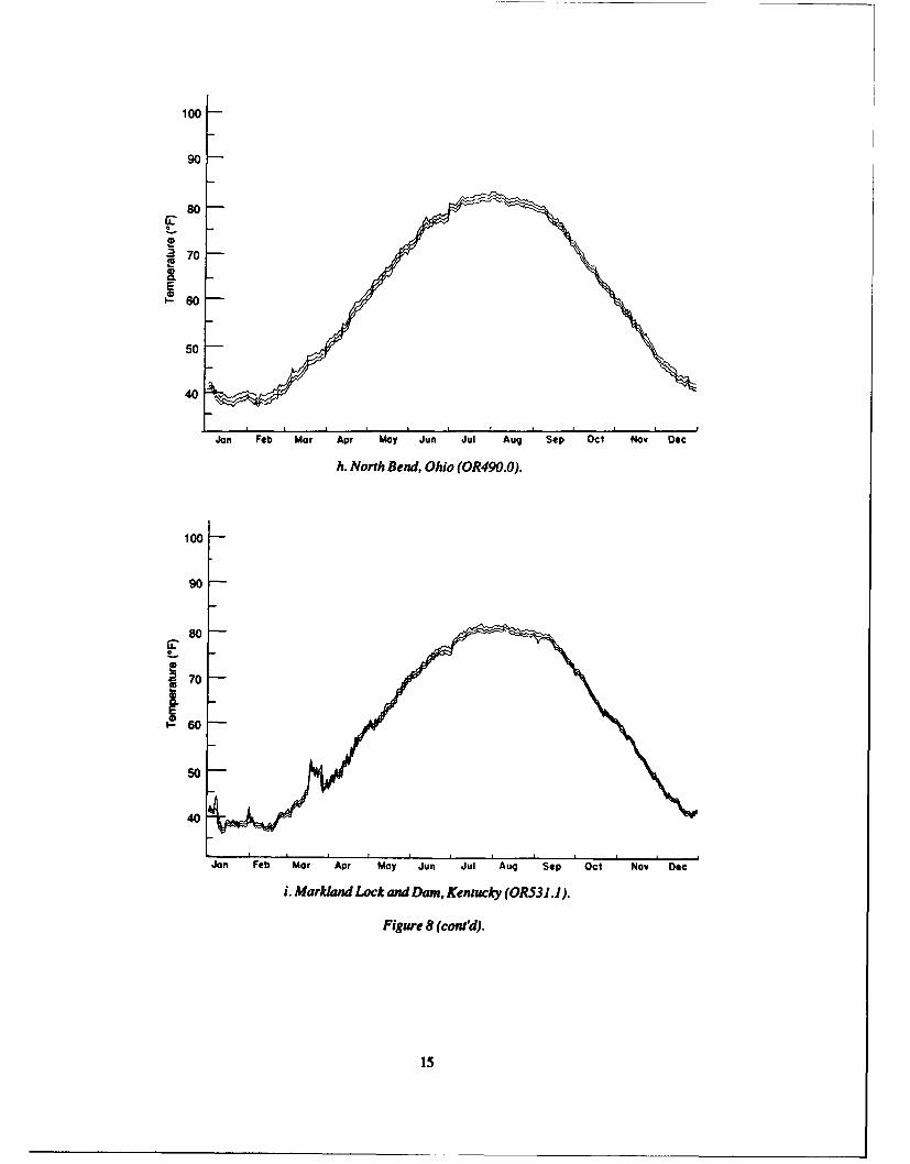
The mean daily average water temperatures (Ohio with those having relatively short records. The longRiver Valley WaterSanitationCommission 1982)mea- period records provide smoother curves and smallersured at 14 sites along the Ohio River (Fig. 6) range daily temperature fluctuations.narrowly from about 56.7°F near the upstream end to Third, although the water temperature records for all61.2*F at Joppa, Illinois (Table 3). The lowest and 14 locations show a minimum during January, they alsohighest mean daily average water temperatures record- indicate a slight rise, which may be the result of theed in the upstream portions of the river (Fig. 7) are occasional "January thaw." There is a second minimumslightly less than those observed downstream, although watertemperature during mid-February, after which thethe difference is less than 50F in both cases. The lowest temperature in the river tends to increase steadily. Thismean daily average is 33.1*F, and the highest mean slight warming in January is not well described by thedaily average is 85.3°F. sinusoidal equation above, and would require higher

The mean daily minimum, average and maximum order harmonics to reproduce.temperatures plotted for the 14 sites (Fig. 8) show sev-eral features. First, the annual temperature curves fol- River icelow a sinusoidal pattern, with the lowest temperatures in Ice cover on the Ohio River can be quite dynamic,January and February and the highest in July and Aug- forming and breaking up very quickly. It is generatedust. These high and low periods reveal the slight time principally by the extraction of heat from the river itself,lag experienced between air and water temperature but additional ice also. enters the Ohio from its tributar-peaks. ies. Ice can cause many navigation problems, especially

Second, the water temperature (T.) variations for the at locks and dams, where the ice impedes lockages andOhio River Valley Sanitation Commission sites can be the operation of gates, and in general causes hardshipsdescribed by to personnel and equipment (Zufelt and Calkins 1985).

If the ice becomes excessive or sufficiently thick, it canTa Tm + alsin -2-t + 0) (3) impede ship passage nearly everywhere during severe

T winters, especially at river bends and at lock and damwhere Tm = long-term average temperature (°F) sites.

9

40

22

0, 0

211 0

2 C

0 -CY OCt

0 U r

*1z -e -M

0 0

3- CD -i2

zU0-

0 8..

-, 0

100

(T) (C)

S I I I I ' I90-

_30 HgeoMen Daily Average

80 - 3

Z70-i 20-

E

60 - Mean Daily Average

50- 10-

40- Lowest Mean Daily Average

0 200 400 600 800 1000

Distance (miles)

Figure 7. Long-term water temperatures along the Ohio River (distance scaleshows miles from Pittsburgh, Pennsylvania).

Descriptions of ice conditions throughout the Ohio especially during severe flooding, and from unpub-River are available from Gatto (1988). Ice information lished data (e.g., Gatto and Daly 1986).for selected locations is available from daily navigation The following review of past ice conditions ob-reports for each lock and dan prepared by the Corps of served at Cincinnati is based on data from the Corps ofEngineers (analyzed by Bilello et al. [1988]), from an Engineers (1978) report, and detailed by Daly and Bil-Ohio RiverDivision summaryreport (U.S. ArmyCorps ello (1986).of Engineers 1978) for the Cincinnati area, from news- The longest periods of ice on the river each winterpaper and magazine articles addressing ice conditions, (i.e., 40 days or more of observed ice per season) were

100

90

80

0

60

50

40

Jan Feb Mar Apr May Jun Jul Aug Sep Oct Nov Dee

a. South Heights, Pennsylvania (CR015.2).

Figure 8. Annual distribution of mean daily minimum, average and maximum water temperaturesat the Ohio River Valley Water Sanitation Commission water temperature sites.

11

100

90

80

0

a70CL

60

50

40

Jon Feb Mar Apr May Jun Jul Aug Sep Oct Nov Doec

b. East Liverpool, Ohio (CR040.2).

100

90

80

0a 70 BC-P60

50

40

Jan Feb Mar Apr May Jun Jul Aug Sep Oct Nov Dec

c. Shadyside, Ohio (CR102.4).

Figure 8 (cont'd). Annual distribution of mean daily minimum, average and maximum watertemperatures at the Ohio River Valley Water Sanitation Commission water temperature sites.

12

100

90

80LL

70

EI-60

50

40

Jan Feb Mar Apr May Jun Jul Aug Sep Oct Nov Dc

d. Addison, Ohio (CR260.0).

100

90

80

0

E1! 60

50

40

Jan Feb Mar Apr May Jun Jul Aug Sep Oct Nov Doc

e. Gallipolis Lock and Damn, Ohio (CR279.2).

Figure 8 (cont'd).

13

100

90

80

70

a -,1E2 60

50

40

Jan Feb Mar Apr May Jun Jul Aug Sep Oct Nov Dec

f. Huntington, West Virginia (CR306.9).

100

90

80

70

1! 60

50

40

Jon Feb Mar Apt May Jun Jul Aug Sep Oct Nov Dec

g. Cincinnati Water Works, Ohio (CR462.8).

Figure 8 (cont'd). Annual distribution of mean daily minimum, average and maximum watertemperatures at the Ohio River Valley Water Sanitation Commission water temperature sites.

14

100

90

80

'~70

I-60

50

40

Jan Feb Mar Apr May Jun Jul Aug Sep Oct Nov Dec

h. North Bend, Ohio (0R490.O).

100

90

so

0

160

50

40

Jan Feb Mar Apr May Jun Jul Aug Sep Oct Nov- Dec

i. Markiand Lock and Dam, Kentucky (0R531.)).

Figure 8 (cont'd).

15

100i

90

80

0-- 70

Ei- 60

50

40

Jon Feb Mar Apr May Jun Jul Aug Sep Oct Nov Dec

j. Louisville, Kentucky (CR600.6).

100

90

80

0

0

40

Jon Feb Mar Apr May Jun Jul Aug Sep Oct Nov Dec

k. West Point, Kentucky (CR625.9).Figure 8 (cont'd). Annual distribution of mean daily minimum, average and maximum watertemperatures at the Ohio River Valley Water Sanitation Commission water temperature sites.

16

100

90

80

0

2.

EI- 60

50

40

Jon Feb Mar Apr May Jun Jul Aug Sep Oct Nov Dec

I. Cannelton, Indiana (CR720.7).

100

90

80

70

0

50

40

Jon Feb Mar Apr May Jun Jul Aug Sep Oct No Dec

m. Evansville, Indiana (0R791.5).

Figure 8 (contd).

17

100

90

80

70 70-

12 60

500

Jon Feb Mor Apr Moy Jun Jul Aug Sep Oct Nov Dec

n. Joppa, Illinois (CR952.3).

Figure 8 (contd). Annual distribution of mean daily minimum, average and maximum watertemperatures at the Ohio River Valley Water Sanitation Commission water temperature sites.

observed during 13 winters prior to 1940-41, with only 112 years of record (Fig 11). Average monthly temper-two other such events (during the very cold winters of ature values greater than or equal to 32°F (i.e., zero1976-77 and 1977-78) since that time (Fig. 9 and 10). FDDs) were recorded during 31 of the 112 winters, asNo ice was observed on the river during 17 of the 66 compared to the 15 winters when the total seasonalyears of record prior to 1940-41 (or 26% of the time), FDDs exceeded 300 (shown by specific months, D-whereas no ice was noted during 20 of the following 46 December, J-January, F-February). During these 15winter seasons (or 43% of the time). winters, January most often saw the greatest accumula-

A gradual, erratic decrease in ice on the Ohio River tion of FDDs.at Cincinnati from about 1902 to 1975 is shown by the Overlongerconsecutiveperiods(i.e.,thetrendshownsequential five-year average ice values (Fig. 10). This by the five-year average increments), the FDDs re-general reduction in ice coincides somewhat withwarmer vealedearliercold winters between 1874and 1920 (Fig.winters. Minorvariations in the time of thehighandlow 11). Then, except for three or four abnormally coldvalues were noted when the starting point for the five- winters (e.g., December 1935-February 1936), thisyear averages was shifted two or three seasons forward, cold period was followed by a warmer trend that lastedbut the overalltrend forthe fullrecordremainedsimilar. until about 1956. Between 1957 and 1986, the area ex-When ten-year averages were used, the high and low perienced two significant intervals of cold winters. Thevalues became less distinct, first interval extended mostly from 1957 to 1971, and

In an investigation ofthe effect of the winter temper- the second from 1976 to the winter of 1985-86. Theseature regimes on the river ice, Daly and Bilello (1986) two cold periods were separated by four consecutivecomputed a freezing degree-day (FDD)* index for warm winters, 1971-72 to 1974-75.Cincinnati. This value provides arealistic account of the The relationship between the number of days withlength or intensity of the freezing regime for an area. ice each winter and the concurrent total seasonal FDDsThe various periods of warmer and colder winters were was determinedby computing their ratios. For example,found to be randomly distributed throughout the entire during the winter of 1874-75, ice on the Ohio River at

Cincinnati was observed on 43 days, and the total of the

71e hug degree-a for my. owday e de FDDs for that winter was 311; 43 dividedby 311 resultsbetweem the avenge daily air temperutm and 32OF (U.S. Army nd in a ratio of 0.138. Similar ratios were computed for allAir FArce 1966). For example: 32F-(-3F) - 35 fheezing degree 112 winters. Included in Figure 12 are 1) those wintersdays- when ice was reported but the total FDDs was zero

18

40

U

0 YD

U.U

00

0 0C .11 I Jr

'iiu~II~

- Iz

0n fa 0 in 0I-

019

80. No ice observed.

o---o Trace of 5-winter averages

UH

'a 60-

0

40--

0

0 --0

E

1875 '85 '95 1905 '15 25'55 '65 '75 '85Winter Periods

Figure 10. Total number of days when ice was observed on the Ohio River at Cincinnatiduring each winter.

80 C No overage monthly temperature less than 32*F,

o Average of 5 winters.D. J, F: Month of lowest temperatures.

.

6 -o

" -,

40

I. / 0

875 '85 '95 9 D '15 '25 '35 '45 '55 '65 '75 '85Winter Periods

Figure 11. Total seasonalfreezing degree-days at Cincinnati during each winter.

(indicated as solid squares), 2) three winters when the observed ice and no FDDs (indicated as solid circles),

ratio value exceeded 0.6 (indicated as open triangles; and 5) a dashed line showing the average ratio of all theowing to apparent observation errors, these three values values for each consecutive 10-year interval (i.e., start-were considered unrepresentative and therefore were ing with 1874-75 through 1883-84).not used in the study), 3) those winters with some The winter-to-winter ratios shown in Figure 12 re-

recorded FDDs but no days with observed ice (indicated veal considerable variance. Omitting those winters with

as inverted solid triangles), 4) those winters with no symbols, we see that the ratios range from greater than

20

0.6

0.4

02

0-

1875 '815 95 1905 15 '25 35 45 55 6 5 8

Winter Periods

Figure 12. Ratio of total number of days of ice on the Ohio Riverdivided by the total seasonal

freezing degree-days for each winter.

S I I I r I i I0.8-

0.6

0

.0 0.40

0.20~~Trand

0 100 200 300 400 500xlO3

Population of Cincinnoti

Figure 13. Relationship between ratio values (of observed ice versus

freezing degree-days) and population trends at Cincinnati, Ohio, since

1900.

0.4 during the early part of the record to less than 0. 1 and 0.04. Of greater significance, though, is the marked

during the later. The dashed line joining the sequential decrease in the value, as well as the increase of the

10-year average ratios, however, included six consecu- number of years with FDDs but no observed ice (indi-

tive average values of between 0.1 and 0.2 for the win- cated by the inverted solid triangles) after the winter of

ters extending from 1884-85 to 1943-44. Incidentally, 1941-42. We attribute these reductions in ice on the

an investigationofaverage five-yearratiovalues showed river in part to the construction of high-lift locks and

a more erratic overall trend. The average value for the dams, the increase of navigation on the river, and the

33 winters during which ratios were computed in this general development of the Ohio River valley.

period was 0.17, with highest and lowest ratios of 0.46 A good index of watershed development can be

21

determined from the region's increase in population. In metropolitan areas are reflections of the well document-fact, population can be correlated with several hydro- ed"heat island" phenomenon (Terjung 1970). Freezinglogic parameters (Daly and Peters 1979). As arepresen- air temperatures along the river normally occur intative population of the Ohio River Valley, the census December (Fig. 15b) at many Pennsylvania and Ohiorecords for Cincinnati, Ohio, were examined. The pop- locations. In January (Fig. 15c), freezing temperaturesulation of Cincinnati has increased more orless linearly occur over most of the region, except for the extremesince 1900, from about 4000 to 400,000. The decrease southwest and isolated areas further upstream. In Feb-in the computed ratios of observed ice to freezing ruary (Fig. 15d), the average freezing isoline is locateddegree-days during this period paralleled this general slightly northeast of its January location, and meltingincrease in population (Fig. 13). It is not possible to commences along areas south of the line. The reportedprove direct cause and effect, other than what we have air temperatures for Burgettstown and Waynesburg,suggested above. However, the decrease in the ratio of Pennsylvania (station numbers 15 and 19), appear lowobserved ice to the number of freezing degree-days has and were considered unrepresentative. For example, intaken place during the period of watershed de- January (Fig. 15c) Burgettstown's reported averagevelopment. temperature of 24.80 F is about 2 to 4.5*F lower than

Navigation in the Ohio River has increased substan- nearby stations. Although similar differences in tem-tially over the period of record. In 1930, slightly over 20 perature were found during the other winter months, wemillion tons of freight were shipped over the Ohio made no attempt to explain such anomalies, since thisRiver. In 1974, the amount was nearly 140 million tons would be beyond the scope of this report. Thom'sand was made up largely of coal and coke, with lesser (1968) isolinemapsofthestandarddeviationsofmonthlyamounts ofothercommodities such as petroleum, stone, average temperature for the Ohio River Valley regionsand, gravel, chemicals, iron and steel (U.S. Army range from approximately ±0 to ±3.5°F in November,Engineer Institute for Water Resources 1979). Cargo and from ±0 to ±5.5°F for December through March.carriers travel the Ohio River during the winter, except Examination of the average midwinter air tempera-during the few times of severe ice conditions. Naviga- tures along the valley (Fig. 15c) indicated the existencetion can influence the ice conditions in a navigable of the well-documented association between decreas-waterway such as the Ohio River (Ettema and Huang ing temperatures and increasing elevation. The numer-1985). It has generally been reported that navigation ical relationship, however, for the Ohio River Valleytends to increase ice production by repeatedly creating data appeared to differ from the standard atmosphericopen water areas in which new ice can grow (Sandhurst adiabatic lapse rate of 0.330F decrease in temperature1981). Therefore, it is not likely that the increase in for every 100-ft increase in height. Consequently, anavigation itself has caused the decrease in observed simplified contour map (Fig. 16) using each stationice at Cincinnati. elevation was drawn, which confirmed the generally

uniform increase in elevation upriver with decreasingtemperatures. The numerical relationship between the

WINTER CLIMATE 30-year average January air temperature and the eleva-tions for the 80 stations is presented in Figure 17 and

Air temperature regime for November shows a decrease of about I*F in air temperature forthrough March every 100-ft increase in elevation. The correlation coef-

ficient ris 0.835, and the standard deviation is ±1.7 1*F.30-year average air temperatures The calculated line of best fit is

We used data for 30-year normals (1951-80) from80 weather stations along the Ohio River Valley adja- y = -0.0095x + 36.6 (4)cent to or within 50 miles of the river (Fig. 14, Table 4)in a survey ofthe winterclimate forthe region. Analysis where x = station elevation (in feet) and y = averageof the monthly average air temperatures (Fig. 15) pro- January air temperature (degrees Fahrenheit) (i.e., 30-vided the following observations. As expected, during year normal value). The average January air tempera-November through March the temperatures are highest ture was used because it statistically approximates thein southern Illinois and lowest in southwestern Pennsyl- duration and intensity of an average freezing season forvania, ranging from approximately 48 to 400F in No- each location (see Bilello and Appel 1978).vember, 34 to 240 F in January and 48 to 34 0F in March.The increase in average air temperatures down the val- Mean minimum air temperaturesley, except for isolated locations (such as at major cities) As previously noted, the temperatures for Burgetts-is quite uniform. The higher temperatures reported in town and Waynesburg were consistently low in com-

22

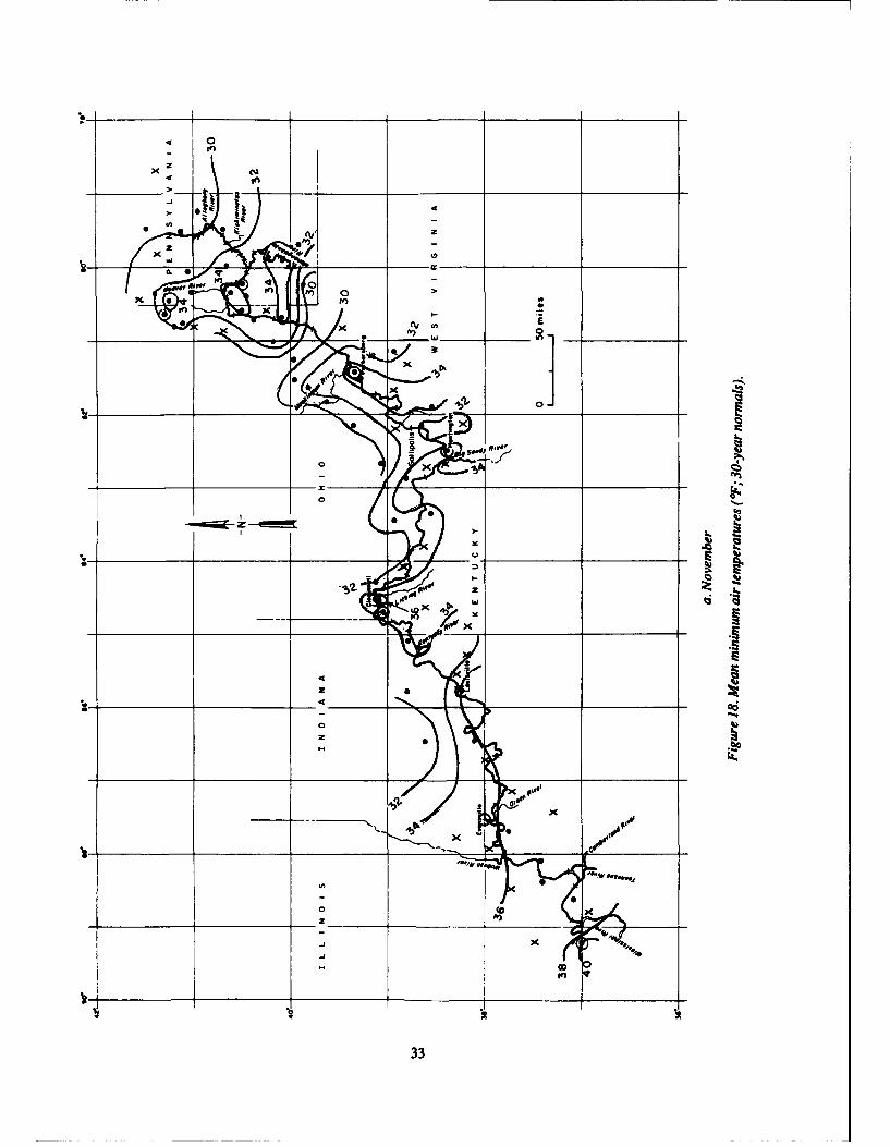
parison with surrounding stations, and therefore, were ated with major rainstorms or rain-on-snow events thatagain ignored. Meanminimumair temperature patterns lead to flooding. Total winter precipitation decreases(Fig. 18) were similar to those for the average monthly from over 20 in. at the southwestern end of the Ohiotemperatures. The highest values occur at the Mississip- River to less than 13 in. in parts of the northeast sectionpiRiverjunctureandthelowest in the headwaters. They of the river valley (Fig. 20).range from approximately 40 to 30OF in November, 26 A visual comparison of the distributions of precipi-to 14OF in January, and 38 to 22°F in March. The entire tation (Fig. 20) and average January air temperaturesarea experiences mean minimum air temperatures be- (Fig, 15c) shows they are similarexcept forfive stationslow freezing during December, January and February, (with mean temperature values below 240 F) locatedsuggesting that ice will form on the river annually. northeast of the Ohio River and in Pennsylvania. ThisThese data by themselves, however, will not provide association make sense physically in that lower-air-reliable predictions of when, where and how much ice temperature regimes contain less atmospheric mois-can be. expected along specific sections of the Ohio ture, and have reduced total precipitation.River for any particular winter. A linear correlation between the average January air

temperature and total winter precipitation for the 75Freezing degree-days stations showed an approximate increase of 0.6 in. of

A combined measure of the duration and magnitude precipitation for every 1 F increase in temperature (Fig.of below-freezing temperatures occurring during any 21). The correlation coefficient r is 0.75, and the stan-given freezing season is defined as the freezing index, dard deviation for the water-equivalent precipitation isand is derived from anaccumulationoffreezingdegree- ±1.44 in. The calculated line of best fit isdays for the season. A freezing degree-day was definedearlier in the Physical Setting and Hydrology section, y = 0.602x - 2.04 (5)and since the index provides an evaluation of both thelength and intensity of the freezing regime, it is worth- where x = average January air temperature (degreeswhile to include it here. Fahrenheit) (i.e., 30-year normal value) andy = average

The mean freezing index, based on the 30-year total water equivalent precipitation (inches) for No-monthly normal air temperatures, was computed for 59 vember through March.of the 80 stations (Table 5, Fig. 19). Three other stations The correlation coefficient for the relationship be-recorded 32.00 F or higher monthly mean normal air tween elevation and decreasing amounts of the totaltemperatures during the winter months. The remaining water-equivalent precipitation recorded from Novem-18 locations did not record any monthly mean normal ber through March was less than that for the relationshipair temperatures of 32°F or lower. The 0 and 50 mean shown in eq 5.freezing index lines (Fig. 19) roughly follow the rivervalley from Evansville, Indiana, to Parkersburg, West Mean annual and monthly maximum snowfallsVirginia. The values then increase rapidly from 100 to Much of the monthly precipitation amounts for No-over 600 mean total freezing degree-days up the valley. vember through March discussed in the previous sec-

This distribution clearly shows that the valley can be tion include the water-equivalent portions of measuredclassified into three general winter temperature re- snowfalls. An examination of the distribution of thegimes. The most severe region lies upstream of thf; con- mean total annual snowfalls and the distributions offluence of the Ohio and Muskingum rivers, where the monthly maximum snowfalls is therefore of interest.mean freezing index values begins to increase rapidly. The mean total annual snowfall amounts increaseA moderate zone extends from that confluence to the from approximately 10 in. at the southwest end of themouth of the Wabash River. The least severe zone is Ohio River Valley to between 25 and 30 in. in thelocated downstream of the Wabash, where no mean vicinity of the Ohio, West Virginia and Pennsylvaniafreezing degree-days are recorded. Although the last borders (Fig. 22). Annual snowfall amounts then in-region is the mildest, river ice could form there or drift crease very rapidly from 35 in. to as high as 60 in. overin from upstream during particularly cold winters. a distance of about 60 miles north of the headwaters of

the Ohio River.Precipitation regime for November The monthly maximum snowfall amounts exhibit anthrough March interesting reverse distribution along the Ohio River

Valley. The 20 in. monthly maximum isoline in theAverage total precipitation southwestern Ohio River region, for example, is 11/2 to

Data on precipitation are extremely important in 2 times greater than the mean annual total value of l0tostudies of winter floods, river stages, ice levels and ice 15 in. An explanation for this is that particular winterjams because ice runs in the winter are usually associ- storms in the warmer (southern) region often contain

23

-x z

-h--i

X N%

)c or- a

ini

-- ii 1-49m!ML

P.-I

LN 4

24

000 In =0m~00 r"M e m e n9

ao 000 G cc ccac0000 0000o00000000000 00 0000 00 000000

;VIA~~ ~ ~ ~ zcnI. Z oo Z obeq V 0 o-

I' SE9 F13.r 1,1

.5en m m m~~uo m -M

I ~ ~=T.g ~ .

C4 3: en~

en 4e4C4 r3.. V 0W 1we.2C -( ne n

a! 0 00-

II00 C 10 - %C IR 4 000 "1 Ii, c"1 0r n0

b, b4 b b

in E 025

0

x 4

0(0

400

V,

414

ax

00

2x

0-0

26

xz

x z

x 40)

3*1

X-

Po -rg

2x

-Ju

27

xz

4L4.

0

Ix.

x~

II.

0

-I-

-JX

28

xzx

x

0 X3

31

__________4 ______e x

\N

zX

22

S ________________ ________________

4

X A~(O4

-4-I

4

x

S

0

1~

a

__________ ___________ ___________ ___________ I3..

____ ____ ____ ____ - ~

____________ ____________ ____________ ____________ 3-

-. 4

40

02

30

00a______ _______ _______ ______________________

400

IL

00 J

00

000

0.

o 00

000

5- 0

a0 0

00_ _ _ _ _ \ . _ _ _ _ _ _%_

31_ _ _ _ __ _ _ - 0

I I I I I I

36-

000 0

00

24 o oo 0

0 00

4000 0 02 00 0 0

0 000 ( y-0.0095x+36.600 8) 0r -0.835

0

~28- % 00 %-, 00

00 000 0

6)0

24 -0 00

10 ? 0

400 800 1200 1600x = Elevation (ft)

Figure 17. Relationship between station elevation (ft) and averageJanuary air temperature (F).

sufficient atmospheric water vapor to produce substan- ample, Bates and Brown 1982). It would be particularlytial snow on a storm-by-storm basis, resulting in occa- pertinent in those areas with "ripe" (near thaw) high-sional high monthly maximum values. But over long density snow packs, and when rapid above-freezingperiods (i.e., on a seasonal basis), the higher air temper- temperature rises and rain occur simultaneously.atures in this area bring rain instead of snow, thus totalannual snowfall amounts are lower. As described in thefollowing discussion, these climatic conditions are re- CONCLUSIONSversed in the northeast region of the river valley.

Both mean annual and monthly maximum snowfall The Ohio River Valley has three physiographicamounts of about 15 to 20 in. are recorded near Louis- regions: the Appalachian Plateau, the Central Lowlandsville, Kentucky, and extend northeastward to Parkers- and the Interior Low Plateau. Long-term average waterburg, West Virginia (Fig. 22). However, upstream in discharge values from aparticularsub-watershed, how-southwestern Pennsylvania, the ratio of average annual ever, follows a fairly consistent relationship regardlessto monthly maximum snowfall amounts is the reverse of the region it is in. This relationship also holds for theof that observed at the southwestern end. In this region Ohio River itself.the monthly maximum values of about 25 to 30 in. are Average discharges forthe Ohio Riverwere found toabout 11/2 to 2 times less than the annual amounts of 50 vary considerably during the year. Maximum discharg-to 60 in. This reversal occurs because of the longer and es and minimum water temperatures normally occur incolder winters experienced in the northeast section of the winter. Frequent and random peak discharges usu-the Ohio River. The numerous individual snowstorms ally come in association with concurrent precipitationin this area produce greater total amounts of snowfall or snowmelt, or both. Major changes in ice conditionsannually than what is generally recorded during any one on the Ohio River, such as ice breakup and rapid move-month. ment, occur during these high discharges.

This snowfall information is useful in the calcula- Although the mean minimum and mean maximumtions of probable river stages and resultant ice jam for- daily water temperatures on the Ohio River are as lowmations caused by runoff from snowmelt (see, for ex- as 33*F and as high as 85°F, respectively, the long-term

32

xz

-4..4

J. rfh

- I

a0

xa

333

C-I-

a Co

C2

-Z-

00

x-------- V4

x z49 i (0

> t~i

0 > *

xx______ _____

0

bl

3c5

x -

0n 0

2*(NJ.2

0C _________ _______ ______________ ______________

* ~ 0

, a,..to,' mfI

x 4,1

0

-Ol

36.

4G

44

C ________ _____ _____ ____________________37_

soo 0

4x E

WI 4

)'o'p

380

4

xzz

0 >

E

I.

p3- -

13

19a

ir-

39a

m ~ F.4 0% C

_e C.- eni q.-:O% C40~ :4~r 0CJ M *(n 00 1-%

I a - cp r - -R I t: - Wt i t-

Ck.

§.q-S-4

04 (4

[-; %nn In00

IfV~~IOC..n' ~~In( IC.0II0 0'C

co V~O C Ie~ICOvC~ C4 gg O 'I

x3w w

40

' I I I

24

0

20 0 00000 0 0

"0. y = 0.602x-2.04 00.75 o o-~~ ~ ~ o8o ° °o 6

0.0CL #>, 0 0 0

a 0 00 0-- 00 O0 0

00

12 -. - - 0 1 1 I24 28 32 36

x = January Air Temperature (OF)

Figure 21. Relationship between average January air temper-ature and total 5-month (Nov through Mar) water equivalentprecipitation.

average value across its entire length only ranges from into the relative importance of each factor with respectabout 56.7 to 61.2 0F. The lower temperatures naturally to the chronological and areal distribution of ice on theexist on the upstream portion of the river, river. The results would give us an improved capability

Analyses of river ice conditions at Cincinnati, Ohio, for predicting ice behavior at specific times and loca-revealed a decline in the amount of ice during the win- tions on the river.ters from 1902 to 1985. The number of days of observed Future research should also consider investigationsice relative to the number of freezing-degree-days has of the most severe winters on record, observed short-also declined during this period, with the most dramatic term periods of extreme cold, and the frequency, inten-decline starting in the 1930s. Reduction in ice amounts sity and distribution of winter air and water tempera-corresponds with the basin development. This relation- turesthroughouttheareaofinterest. Forexample, anothership may result from the changes in the thermal balance form of freezing index that is used in engineering plan-in the river brought about by the increase in heated ning and construction work is the "design freezingdischarges from new power plants along the riverbanks index." For this index, the average value of the air tern-as population increased, and from changes in the stage peratures for the three coldest winters in 10 years, or theand flow regime caused by the construction oflocks and 10 coldest in 30 years, is used. This approach woulddams. Further research is required to quantify the effect account for the extremely cold winters, such as 1976-77of these changes on river ice formation, however, and 1977-78, that were experienced recently in the

Additional detailed studies of the winter climate in eastern half of the U.S. (Kerr 1985). Such records thendirect association with records of ice formation, growth could be compared with historical navigation or lockand decay and river ice levels, ice jams and blockages and dam records, or compared with recent aircraft orare also required. For example, it would be worthwhile satellite imagery data of concurrent ice observations onto select a particular winter with severe ice conditions the Ohio River. The ultimate objective would be toon the Ohio River, and gather all available hydrologic, develop an accurate river ice forecast model using realphysiographic and environmental data recorded during time observed weather patterns and the associated riverthe entire period. An integrated analysis of all of the ice conditions.contributing parameters could provide some insight

41

16-C

.j g4 ~0

E4

11 -

IZI

kI-

04%

42

LITERATURE CITED(1983) Local climatological data, annual summary with

Bates, R. and M. Brown (1982) Meteorological con- comparative data 1982. Asheville, North Carolina: Na-ditionscausingmajoricejam formation and flooding on tional Environmental Data, and Information Service,the Ottauquechee River, Vermont. USA Cold Regions National Climatic Data Center.Research and Engineering Laboratory, Special Report Ohio River Basin Commission (1979) The Ohio River82-6. Basin, the Regional Water and Land Resources Plan.Bielo, N. J. Gagnon and S. Daly (1988) Computer- Cincinnati: Ohio River Basin Commission.generated graphics of river ice conditions. In The Sev- Ohio River Valley Water Sanitation CommissionenthNorthernResearchBasinsSymposiumlWorkshop, (1982) Water Quality Monitoring Strategyfor the Ohio25 May-I June, Iluissat, Greenland. Copenhagen: River and Lower Reaches of Major Tributaries. Cin-Danish Society for Arctic Technology, p. 2 1 1-220. cinnati, Ohio.Bilello, M.A. and G.C. Appel (1978) Analysis of the Sandhurst, J. (1981) Conditions in brash ice-coveredmid-wintertemperature regime and snow occurrence in channels with repeated passages. In Proceedings, 6thGermany. USA Cold Regions Research and Engineer- International Conference on Port and Ocean Engineer-ing Laboratory, CRREL Report 78-21. ing under Arctic Conditions (POAC '81), 27-31 July,Daly, S. and M. Bilello (1986) Analysis of 112 years of Quebec, Canada. Universit6Laval, vol. 1, p. 244-252.ice conditionsobservedontheOhioRiver atCincianati. Stoker, JJ. (1957) Water Waves. New York: Intersci-In Proceedings of the 1986 Annual Meeting, Eastern ence Publishers.Snow Conference, 5-6 June, Hanover, New Hamp- Terjung, W.H. (1970) Urban energy balance climatol-shire, p. 70-79. ogy. The Geographical Review, LX(1), January.Daly, S.F. and J. Peters (1979) Determining peak- Thorn, H.C.S. (1968) Standard deviation of monthlydischarge frequencies in an urbanizing watershed-A average temperature. Silver Springs, Maryland: U.S.case study. In Proceedings of the International Sym- DepartmentofCommerce, Environmental Science Ser-posiumon Urban Storm Runoff, July 23-26,Lexington, vice Administration, ESSA Technical Report EDS-3.Kentucky. University of Kentucky, p. 183-195. Thornbury, W.D. (1965)RegionalGeomorphology ofEttema, R. and H.P. Huang (1985) Ice regrowth and the U.S. New York: J. Wiley and Sons, Inc.brash-ice accumulation in navigation channels--A lit- US. Army and U.S. Air Force (1966) Arctic and sub-erature review. Progress Report for the USA Cold Re- arctic construction, general provisions. U.S. Armygions Research and Engineering Laboratory (unpub- Technical Manual No. 5-8532-1 and U.S. Air Forcelished). Manual No. 88-19, Chapter 1.Gatto, L. (1988) Ice conditions along the Ohio River as U.S. Army Corps of Engineers (1978) Ohio River Di-observed on Landsat images, 1972-1985. USA Cold vision Ice Committee summary report. Cincinnati, Ohio:Regions Research andEngineering Laboratory, Special U.S. Army Engineer Division, Ohio River.Report 88-1. US. Army Corps of Engineers (1981) National wa-Gatto, L. and S. Daly (1986) Ice conditions along the terways study. Fort Belvoir, Virginia: U.S. Army Engi-Allegheny, Monongahela and Ohio rivers, 1983-1984. neer Water Resources Support Center. Institute forUSA Cold Regions Research and Engineering Labo- Water Resources.ratory, Internal Report 930 (unpublished). U.S. Army Corps of Engineers (1979) NationalKerr, ILA. (1985) Wild string of winters confirmed. waterways study, waterways system and commodityScience, 227(1 February): 4686. movement maps.Fort Belvoir, Virginia: U.S. Army En-National Oceanic and Atmospheric Administration gineer Water Resources Support Center. Institute for(1982a) Climatography of the United States No. 60. Water Resources.Climate of Pennsylvania, West Virginia, Ohio, Ken- U.S. Department ofCommerce (1968) Climatic Atlastucky, Indiana and Illinois. Asheville, North Carolina: ofthe United States. Asheville, North Carolina: Nation-Environmental Data Service, National Climatic Center. al Climatic Center.National Oceank and Atmospheric Administration U.S. Geological Survey (1982) Water resources data,(1982b) Climatography of the United States No. 81 (by by states andcontinuous foranumberofyearsofrecord.state). Monthly normals of temperature, precipitation, USGS Water-data report series, prepared in coopera-andheatingandcoolingdegreedays 195 1--80.Asheville, tion with individual states and other agencies.North Carolina: Environmental Data and Information Zufelt, J. and D. Calkins (1985) Survey of ice problemService, National Climatic Center. areas in navigable waterways. USA Cold Regions Re-National Oceanic and Atmopheric Administration search and EngineeringLaboratory, Special Report 85-2.

43

APPENDIX A: DAILY AIR TEMPERATURES, WATER TEMPERATURESAND DISCHARGES AT TWO LOCATIONS ON THE OHIO RIVER

z z

00

U0

-U,4

aijid oLAlo(4) i~id oLAla'A

0 0 0 0

00

o 0

610

0 4

o 0 0 T .

(3.)~~~ ~ ~ ~ ~ siIisue AIo'A 45(. Ijide lo'A

0 00 0§

00

CO

- jii

00No

s4. *Jl4ojidwSL AIlonI O (1 SOfl4Oiedwo. AIIDoa AV

460

1z

00

"00

8 0 o 50As(

0 0

A,

00

000

1 Al02z

siiUdii AUo'~ igidu.

040

00

C', P

CDC

Id 00

0

a 0%

N C

cm I(a. *noJsdwel A IIoo'BAV (3.) eisjOdwos AliICOAV

48

I f

t I-

0 0 0

0 0

o

0 0

U.A

0(

0 0 0 0

(0.) sijfloiedwo±L £1100BAV (3.) sJiDJiedwo± 11 lcaBAV

49

0

t 0

0

2 0

v --

0 0 0 0

00

CD co;Z'

0 0

(3,~) s*jfloiedwog AII00BOAV co) iniciodwel AIlo0BDAV

50

0 0

U)-

0IZ0

z z

00

0~ 0S~J 0Boog~(45 BOO~

00

(,I.) *JflIojodwo. AIIDO3 OAv (.40) sin4Oiedwel AIIo O AV

0 0 0 0 0 0co to 00

II

tC

II-

0,

0 0

gin)sojflDdwoj. AlloaOCAV (3.) siniciedwo. A I foaoAV

51

0 00V W.

00(S/t 95J43SII 0IS/ J;)96100st

ODC

o a

00

o0

zz

00

CY 0

(j)siniOJedwJ.L A I Ia -5A (j* o~fiedwo.L AIIoC 5A

o o 0 0 02

OD.

a

C-i

caa

UJD 0

0 0 0

C L

(s. Sn~o~dej jj 0 ev j* *JIIJ~d.J AIoaOo

( S) il&oJdwej Alloa -OAV (0)sfinpiedwisjA loo0 SDAW

53

'Cc

0 00C-C

sin~iedol AicK (Zi) *n~ojd~u.L Aloo-OA

0 0 0oCD N w z

cyU

0@

( ) inioidwj.L Ajgvo OAV (3.) *Jfl4ojodwoj AIloa*5B,

454

00

00

00

00 8

0S(6/0l) 8JO406SIQ 0 (t 1 weOqSIa]

(j.) gJflieJdwoij £1100 -DAV 0j* 0~ aJ~wJ A0 o0

o U*

- IC

55

0 0

( @~ Jn4Dj~dw. Alloo OAV C.) vjnojojdw9sj AIpoU 5Aj N

00 00 0 0%I I~

0

(~ Joijoadws±L £IIo(]OAV (3.) *jfiividWe.I AIIoabAv'

56

(,I.) sifl4ciedwo. AlIoo BOAV

00

AA

CSC

to cu

(.4.. sifl&oJsduIse. A110a BOAy

0 0 0 0-

woo

0 0

In ri

OD c

57

Form Approved

REPORT DOCUMENTATION PAGE OMB No. 0704-o1WIIJIRPOVNJ IJMI'rairso eOm -- Iv"OI18 W%ss~nsI0 oaoIfht rW R .w~cuf Oti o W"6161110" Ohl, Ineret"amr am~fl dMURK 9@1~os 1" am

Ma~le""nl"0 me dft -~xmd, md a-mo-kdeVWsnmb fthe cbmotkdlon ftL~w wn~malen. Seed oy lnrabure - fsw a coisCin I .,S go for fts bum. to WaWiton0 Nmfatm Sa DiroaMl orkminon operato" eWRoh 1215J&son Daft IHW. 8ub 12D4Alngbn.

VA 2=9430. ad o ft Ofm of Mnmet an &49t. Prwoerk R0on Proi (07040188). Wasngo. DO 20W&

1. AGENCY USE ONLY (Leave blank) 2. REPORT DATE 3. REPORT TYPE AND DATES COVEREDI December 1990

4. TITLE AND SUBTITLE 5. FUNDING NUMBERS

Winter Environment of the Ohio River Valley River !,e i2vianigement ProgramWU: CWIS 32227

6. AUTHORS

Steven F. Daly, Michael A. Bilello and Roy E. Bates

7. PERFORMING ORGANIZATION NAME(S) AND ADDRESS(ES) 8. PERFORMING ORGANIZATIONREPORT NUMBER

U.S. Army Cold Regions Research and Engineering Laboratory72 Lyme Road CRREL Report 90-12Hanover, New Hampshire 03755-1290

9. SPONSORINGIMONITORING AGENCY NAME(S) AND ADDRESS(ES) 10. SPONSORING/MONITORINGAGENCY REPORT NUMBER

Office of the Chief of EngineersWashington, D.C. 20314-1000

11. SUPPLEMENTARY NOTES

12a. DISTRIBUTIONIAVAILABILITY STATEMENT 12. DISTRIBUTION CODE

Approved for public release; distiibution is unlimited.

Available from NTIS, Springfield, Virginia 22161.

13. ABSTRACT (Maxwmum 200 wmo

A general survey of the winter environment of the Ohio River Valley that is relevant to river ice formation is described. Includedare hydrologic, hydraulic and climatic conditions. The long-term monthly discharges steadily increase on the Ohio Riverthroughout the winter season. Inspection of the discharges for each day shows that it has a large short-term variability duringthe winter, with peaks being four to six times the base flow, and generally coinciding with higher air temperatures. River watertemperatures follow a yearly cycle that is can be closely described by a sinusoidal curve. The river water temperatures have theirminimum in January, and also exhibit January "thaws." Ice conditions on the Ohio River are quite variable. The number of dayswith ice each winter has gradually and erratically decreased from 1902 to 1975.The cause of this decrease cannot be determined,but there is a direct correlation with watershed development, as indicated by watershed population. Average air temperaturesshow a good correlation with elevation. Other points discussed are mean minimum air temperatures, freezing-degree days andprecipitation.

14. SUBJECT TERMS 15. NUMEgFS PAGES

Climate Ohio River Winter environment I& PRICE CODEIce River ice

17. SECURFITY CLASSIFICATION IS. SECURITY CLASSIFICATION 19. SECURITY CLASSIFICATION 20. LIMITATION OF ABSTRACTOF REPORT OF THIS PAGE OF ABSTRACT

UNCLASSIFIED UNCLASSIFIED UNCLASSIFIED UL

MON 754010-2.6 Stndard Form 2M (Rev. 2.69)U. S. GOVERNMENT PRINTING OFFICE: 1991--500-063--22058 Pft bl AND VDS.Z

se102