1 Crustal and uppermost mantle structure in the central US 1 encompassing the Midcontinental Rift 2 Weisen Shen 1 , Michael H. Ritzwoller 1 , and Vera Schulte-Pelkum 2 3 1- Department of Physics, University of Colorado at Boulder, Boulder, CO 80309-0390 4 2 - Cooperative Institute for Research in Environmental Sciences and Department of Geological 5 Sciences, University of Colorado at Boulder, Boulder, CO 80309-0390 6 Abstract 7 Rayleigh wave phase velocities across the western arm of the Midcontinent Rift (MCR) 8 and surrounding regions are mapped by ambient noise eikonal tomography (8-40 sec) and 9 teleseismic Helmholtz tomography (25 – 80 sec) applied to data from more than 120 10 Earthscope/USArray stations across the central US. Back-azimuth independent receiver 11 functions also are computed for those stations using a harmonic stripping technique. A 12 joint Bayesian Monte-Carlo inversion method is applied to generate 3-D posterior 13 distributions of shear wave speeds (Vs) in the crust and uppermost mantle to a depth of 14 about 150 km, providing a synoptic view of the seismic structure of the MCR and its 15 adjacent tectonic blocks. Three major structural attributes are identified: (1) There is a 16 high correlation between the long wavelength gravity field and shallow Vs structure, 17 although the MCR gravity high is obscured by clastic sediments in the shallow crust. (2) 18 Thick crust (>47 km) underlies the MCR, but structure near the Moho varies along the 19 rift. (3) Crustal shear wave speeds vary across the Precambrian sutures (e.g., Great Lakes 20 Tectonic Zone, Spirit Lakes Tectonic Zone). The first observation is consistent with an 21 upper crustal origin to the MCR gravity anomaly as well as other anomalies in the region. 22 The thickened crust beneath the MCR is evidence for post-rifting compression with 23 pure-shear deformation of the crust. The third observation reveals the importance of 24 Precambrian sutures in the subsequent tectonic evolution of the central US and in 25 contemporary seismic structure. 26
Transcript
1
Crustal and uppermost mantle structure in the central US 1
encompassing the Midcontinental Rift 2
Weisen Shen1, Michael H. Ritzwoller
1, and Vera Schulte-Pelkum
2 3
1- Department of Physics, University of Colorado at Boulder, Boulder, CO 80309-0390 4
2 - Cooperative Institute for Research in Environmental Sciences and Department of Geological 5
Sciences, University of Colorado at Boulder, Boulder, CO 80309-0390 6
Abstract 7
Rayleigh wave phase velocities across the western arm of the Midcontinent Rift (MCR) 8
and surrounding regions are mapped by ambient noise eikonal tomography (8-40 sec) and 9
teleseismic Helmholtz tomography (25 – 80 sec) applied to data from more than 120 10
Earthscope/USArray stations across the central US. Back-azimuth independent receiver 11
functions also are computed for those stations using a harmonic stripping technique. A 12
joint Bayesian Monte-Carlo inversion method is applied to generate 3-D posterior 13
distributions of shear wave speeds (Vs) in the crust and uppermost mantle to a depth of 14
about 150 km, providing a synoptic view of the seismic structure of the MCR and its 15
adjacent tectonic blocks. Three major structural attributes are identified: (1) There is a 16
high correlation between the long wavelength gravity field and shallow Vs structure, 17
although the MCR gravity high is obscured by clastic sediments in the shallow crust. (2) 18
Thick crust (>47 km) underlies the MCR, but structure near the Moho varies along the 19
rift. (3) Crustal shear wave speeds vary across the Precambrian sutures (e.g., Great Lakes 20
Tectonic Zone, Spirit Lakes Tectonic Zone). The first observation is consistent with an 21
upper crustal origin to the MCR gravity anomaly as well as other anomalies in the region. 22
The thickened crust beneath the MCR is evidence for post-rifting compression with 23
pure-shear deformation of the crust. The third observation reveals the importance of 24
Precambrian sutures in the subsequent tectonic evolution of the central US and in 25
contemporary seismic structure. 26
2
1. Introduction 27
The most prominent gravity anomaly in the central US [Woollard and Joesting, 1964] is a 28
2000-km-long gravity high with two arms merging at Lake Superior and extending 29
southwest to Kansas and southeast into Michigan. This anomaly has been determined to 30
mark a late Proterozoic tectonic zone [Whitmeyer and Karlstrom, 2007]. Because of the 31
existence of mantle-source magmatism and normal faults found along the anomaly, it has 32
been generally accepted that this anomaly resulted from a continental rifting episode and 33
as a consequence is known as the Midcontinent Rift system (MCR) [Schmus, 1992] or 34
Keweenawan Rift system. Geochronological evidence shows that the rift initiated at 35
about 1.1 Ga and cut through several crustal provinces [Hinze et al., 1997]. Although 36
various geological and seismic studies have focused on the rift [Hinze et al., 1992; 37
Mariano and Hinze, 1994; Woelk and Hinze, 1991; Cannon et al., 1989; Vervoort et al., 38
2007; Hollings et al., 2010; Hammer et al., 2010; Zartman et al., 2013], the mechanisms 39
behind the opening and rapid shut down of the rift are still under debate due to lack of 40
information. Fundamental questions, therefore, remain as to the nature and origin of the 41
rift system [Stein el al., 2011]. 42
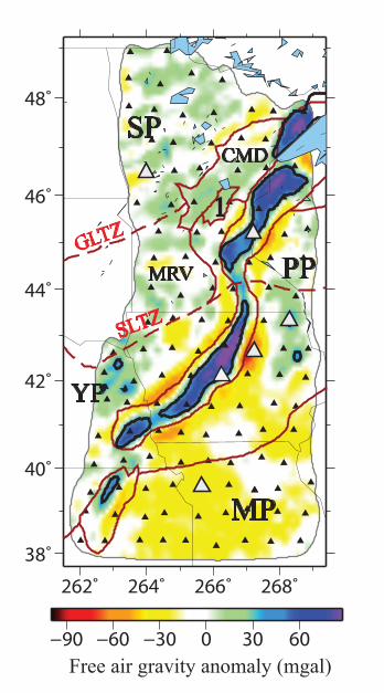
Figure 1 outlines the location of the western arm of the MCR and its neighboring 43
geological provinces. The MCR can be thought of as being composed of three large-scale 44
components: the western arm through Minnesota, Iowa, and Kansas; the Lake Superior 45
arm; and the eastern arm through Michigan. Our focus here is on the western arm. A free 46
air gravity high defines its location (see 40 mgal anomaly contour in Fig. 1), but divides it 47
further into three segments: a northern one extending from near the south shore of Lake 48
Superior along the Wisconsin-Minnesota boundary, a southern one extending from 49
northeastern to southeastern Iowa, and a small segment in Nebraska and Kansas. 50
Marginal gravity minima flank the MCR and have been interpreted as a signature of 51
flanking sedimentary basins [Hinze et al., 1992]. Gravity decreases broadly from 0 - 30 52
3
mgal in the north to -30 mgal in the south. Whether and how these gravity features relate 53
to the structure of the crust and uppermost mantle is poorly understood. 54
The western arm of the MCR remains somewhat more poorly characterized than the Lake 55
Superior component of the MCR due to a veneer of Phanerozoic sediments [Hinze et al., 56
1997]. About two decades ago active seismic studies were performed from northeastern 57
Wisconsin to northeastern Kansas [Chandler et al., 1989; Woelk and Hinze, 1991] that 58
revealed a structure similar to the Lake Superior component [Hinze et al. 1992]. These 59
similarities include crustal thickening to more than 48 km and high-angle thrust faults 60
that appear to be reactivated from earlier normal faults. Cannon [1994] attributed these 61
features to a post-rifting compressional episode during the Grenville orogeny. 62
The MCR cuts across a broad section of geological provinces of much greater age. The 63
Superior segment of the MCR is embedded in the Archean Superior Province (SP, 2.6-3.6 64
Ga), which continues into Canada. In Minnesota, this province is subdivided by the Great 65
Lakes Tectonic Zone (GLTZ) west of the MCR into the 2.6-2.75 Ga Greenstone-Granite 66
Terrane in the north, and the 3.4-3.6 Ga Gneiss Terrane or “Minnesota River Valley 67
Sub-Province” (MRV) in the south [Sims and Petermar, 1986]. During the 68
Paleoproterozoic (1.8-1.9 Ga), the Penokean Province (PP) is believed to have been 69
accreted to the southern edge of the Superior Province, adding vast foreland basin rocks 70
and continental rocks along its margin. This is marked as a “craton margin domain 71
(CMD)” [Holm et al., 2007] in Figure 1. From 1.7-1.8 Ga, the Yavapai province was 72
added to the southern Minnesota River Valley and the Penokean provinces, which drove 73
overprinting metamorphism and magmatism along the continental margin to the north. 74
The East-Central Minnesota Batholith (“1” in Fig. 1) is believed to have been created 75
during this time [Holm et al., 2007] and this accretion produced the continental suture 76
known as the Spirit Lake Tectonic Zone (SLTZ). Later (1.65-1.69 Ga), the Mazatzal 77
Province (MP) was accreted to the Yavapai Province, producing another metamorphic 78
episode south of the Spirit Lake Tectonic Zone. Overall, the 1.1 Ga rift initiated and 79
4
terminated in a context provided by geological provinces ranging in age from 1.6 to 3.6 80
Ga. During the Phanerozoic, this region suffered little tectonic alteration. 81
In this paper, we aim to produce an improved, uniformly processed 3D image of the crust 82
and uppermost mantle underlying the western arm of the MCR and surrounding 83
Precambrian geological provinces and sutures. The purpose is to determine the state of 84
the lithosphere beneath the region using a unified, well-understood set of observational 85
methods. We are motivated by a long list of unanswered questions concerning the 86
structure of the MCR, including the following. (1) How are observed gravity anomalies 87
related to the crustal and uppermost mantle structure of the region, particularly the 88
gravity high associated with the MCR? (2) Is the crust thickened (or thinned) beneath the 89
MCR, and how does it vary along the strike of the feature? (3) Is the MCR structurally a 90
crustal feature alone or do remnants of its creation and evolution extend into the upper 91
mantle? (4) Are the structures of the crust and uppermost mantle continuous across 92
sutures between geological provinces or are they distinct and correlated with such 93
provinces? 94
Since 2010, the Earthscope/USArray Transportable Array (TA) left the tectonic western 95
US and rolled over the region encompassing the western arm of the MCR, making it 96
possible to obtain new information about the subsurface structure of this feature. The 97
earlier deployment of USArray stimulated the development of new seismic imaging 98
methods. This includes ambient noise tomography [e.g., Shapiro et al., 2005; Lin et al. 99
2008; Ritzwoller et al., 2011] performed with new imaging methods such as eikonal 100
tomography [Lin et al., 2009] as well as new methods of earthquake tomography such as 101
Helmholtz tomography [Lin and Ritzwoller, 2011] and related methods [e.g., Pollitz, 102
2008; Pollitz and Snoke, 2010]. New methods of inference have also been developed 103
based on Bayesian Monte Carlo joint inversion of surface wave dispersion and receiver 104
function data [Shen et al., 2013a] that yield refined constraints on crustal structure with 105
realistic estimates of uncertainties. The application of these methods together have 106
5
produced a higher-resolution 3-D shear velocity (Vs) model of the western US [Shen et 107
al., 2013b] with attendant uncertainties and have also been applied on other continents 108
[e.g., Zhou et al., 2011; Zheng et al., 2011; Yang et al., 2012; Xie et al., 2013]. In this 109
paper, we utilize more than 120 TA stations that cover the MCR region to produce 110
high-resolution Rayleigh wave phase velocity maps from 8 to 80 sec period by using 111
ambient noise eikonal and teleseismic Helmholtz tomography. We then jointly invert 112
these phase velocity dispersion curves locally with radial component receiver functions to 113
produce a 3-D Vsv model for the crust and uppermost mantle beneath the western MCR 114
and the surrounding region. 115
2. Data Processing 116
The 122 stations used in this study are shown in Figure 1 as black triangles, which evenly 117
cover the study area with an average inter-station distance of about 70 km. (Stations at 118
which we present example results are identified with larger white triangles in Figure 1, 119
and their names and locations are presented in Table 1.) Based on this station set, we 120
construct surface wave dispersion curves from ambient noise and earthquake data as well 121
as receiver functions. Rayleigh wave phase velocity curves from 8 to 80 sec period are 122
taken from surface wave dispersion maps generated by eikonal tomography based on 123
ambient noise and Helmholtz tomography based on teleseismic earthquakes. We also 124
construct a back-azimuth independent receiver function at each station by the harmonic 125
stripping technique. Details of these methods have been documented in several papers 126
[eikonal tomography: Lin et. al., 2009; Helmholtz tomography: Lin and Ritzwoller et al., 127
2011; harmonic stripping: Shen et al., 2013a] and are only briefly summarized here. 128
2.1. Rayleigh wave dispersion curves 129
We measured Rayleigh wave phase velocities from 8 to 40 sec period from the ambient 130
noise cross-correlations based on the USArray TA stations available from 2010 to May 131
2012. We combined the 122 stations in the study area with the TA stations to the west of 132
6
the area [Shen et al. 2013b] in order to increase the path density. The ambient noise data 133
processing procedures are those described by Bensen et al. [2007] and Lin et al. [2008], 134
and produce more than 10,000 dispersion curves in the region of study. At short periods 135
(8 to 40 sec), eikonal tomography [Lin et al., 2009] produces Rayleigh wave phase 136
velocity maps with uncertainties based on ambient noise (e.g., Fig. 2a-c). For longer 137
periods (25 to 80 sec), Rayleigh wave phase velocity measurements are obtained from 138
earthquakes using the Helmholtz tomography method [Lin and Ritzwoller, 2011]. A total 139
of 875 earthquakes between 2010 and 2012 with Ms > 5.0 are used, and on average each 140
station records acceptable measurements (based on a SNR criterion) from about 200 141
earthquakes for surface wave analysis. Example maps are presented in Figure 2d,e. In the 142
period band of overlap between the ambient noise and earthquake measurements (25 to 143
40 sec), there is strong agreement between the resulting Rayleigh wave maps (Fig. 2f). 144
The average difference is ~ 0.001 km/sec, and the standard deviation of the difference is 145
~ 0.012 km/sec, which is within the uncertainties estimated for this period (~0.015 146
km/sec). 147
At 10 sec period, at which Rayleigh waves are primarily sensitive to sedimentary layer 148
thickness and the uppermost crystalline crust, a slow anomaly is seen in the gap between 149
the northern and southern MCR, and runs along the flanks of the MCR, particularly in the 150
south. Wave speeds are high north of the Great Lakes Tectonic Zone (GLTZ) and average 151
in the Mazatzal Province. Between 20 and 40 sec, the most prominent feature is the low 152
speed anomaly that runs along the MCR, as was also seen by Pollitz and Mooney [2013]. 153
This indicates low shear wave speeds in the lower crust/uppermost mantle and/or a 154
thickened crust beneath the MCR. Higher wave speeds at these periods appear mostly 155
north of the Great Lakes Tectonic Zone. At longer periods, the anomaly underlying the 156
MCR breaks into northern and southern parts and the lowest wave speeds shift off the rift 157
axis near the southern MCR. With these Rayleigh wave phase speed dispersion maps at 158
periods between 8 and 80 sec, we produce a local dispersion curve at each station 159
7
location. For example, the local Rayleigh wave phase velocity curve with uncertainties at 160
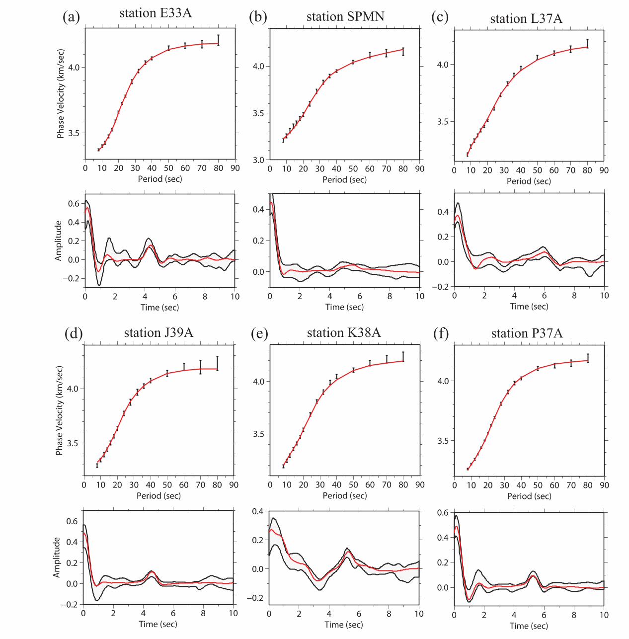
station E33A in the southern Superior Province is shown in Figure 3a with black error 161
bars. Other example Rayleigh wave curves are presented in Figure 3b-f. 162
2.2 Receiver function processing 163
The method we use to process receiver functions for each station is described in detail in 164
Shen et al. [2013b]. For each station, we pick earthquakes from the years 2010, 2011 and 165
2012 in the distance range from 30° to 90° with mb > 5.0. We apply a time domain 166
deconvolution method [Ligorria and Ammon, 1999] to each seismogram windowed 167
between 20 sec before and 30 sec after the P-wave arrival to calculate radial component 168
receiver functions with a low-pass Gaussian filter with a width of 2.5 s (pulse width ~ 1 169
sec), and high-quality receiver functions are selected via an automated procedure. 170
Corrections are made both to the time and amplitude of each receiver function, 171
normalizing to a reference slowness of 0.06 sec/km [Jones and Phinney, 1998]. Finally, 172
only the first 10 sec after the direct P arrival is retained for further analysis. We compute 173
the azimuthally independent receiver function, R0(t), for each station by fitting a 174
truncated Fourier Series at each time over azimuth and stripping the azimuthally variable 175
terms using a method called “harmonic stripping” by Shen et al. [2013b]. This method 176
exploits the azimuthal harmonic behavior in receiver functions (e.g., Girardin and Farra, 177
1998; Bianchi et al., 2010). After removing the azimuthally variable terms at each time, 178
the RMS residual over azimuth is taken as the 1σ uncertainty at that time. 179
On average, about 72 earthquakes satisfy the quality control provisions for each station 180
across the region of study, which is about half of the average number of similarly high 181
quality recordings at the stations in the western US [Shen et al., 2013b]. This reduction in 182
the number of accepted receiver functions results primarily from the distance range for 183
teleseismic P (30o to 90
o), which discards many events from the southwest Pacific (e.g., 184
Tonga). The number of retained earthquakes varies across the region of study, being 185
highest towards the southern and western parts of the study region and lowest towards the 186
8
north and east. At some stations there are as few as 21 earthquake records retained and 187
receiver functions at 15 stations display a large gap in back-azimuth, which prohibits 188
estimating stable, azimuthally-independent receiver functions. For these stations, we use 189
a simple, directly-stacked receiver function to represent the local average. Overall, the 190
quality of the resulting azimuthally independent receiver functions is significantly lower 191
than observed across the western US by Shen et al. [2013a,b] where more than 100 192
earthquakes are typically retained for receiver function analysis. 193
Examples of receiver functions at six stations in the MCR region are shown in Figure 3 194
as parallel black lines that delineate the one standard deviation uncertainty at each time. 195
At station E33A (Fig. 3a) in the southern Superior Province, a clear Moho conversion 196
appears at ~ 4.3 sec after the direct P arrival, which indicates a distinct, shallow (~ 35 km) 197
Moho discontinuity. In contrast, at station SPMN in the northern MCR (Fig. 3b) only a 198
subtle Moho Ps conversion is apparent, which suggests a gradient Moho beneath the 199
station. In the southern MCR, the receiver function at station L37A (Fig. 3c) has a strong 200
Moho Ps signal at ~ 6 sec, implying the Moho discontinuity is at over 45 km depth. At 201
station J39A to the east of the MCR (Fig. 3d), a Ps conversion at ~4.5 sec is observed, 202
indicating a much thinner crust. At K38A, which is located in the gravity low of the 203
eastern flank of the southern MCR (Fig. 3e), a sediment reverberation appears after the P 204
arrival. In the Mazatzal Province at station P37A (Fig. 3f) a relatively simple receiver 205
function is observed with a Ps conversion at ~ 5.3 sec, indicative of crust of intermediate 206
thickness in this region. 207
3. Construction of the 3-D model from Bayesian Monte Carlo joint inversion 208
Here we briefly summarize the joint Bayesian Monte Carlo inversion of surface wave 209
dispersion curves and receiver functions generated in the steps described in section 2. A 210
1-D joint inversion of the station receiver function and dispersion curve is performed on 211
the unevenly distributed station grid and then the resulting models from all stations are 212
interpolated into the 3-D model using a simple kriging method, as described by Shen et al. 213
9
[2013b]. 214
3.1 Model space and prior information 215
We currently only measure Rayleigh wave dispersion, which is primarily sensitive to Vsv, 216
so we assume the model is isotropic: Vsv=Vsh=Vs. The Vs model beneath each station is 217
divided into three principal layers. The top layer is the sedimentary layer defined by three 218
unknowns: layer thickness and Vs at the top and bottom of the layer with Vs increasing 219
linearly with depth. The second layer is the crystalline crust, parameterized with five 220
unknowns: four cubic B-splines and crustal thickness. Finally, there is the uppermost 221
mantle layer, which is given by five cubic B-splines, yielding a total of 13 free 222
parameters at each location. The thickness of the uppermost mantle layer is set so that the 223
total thickness of all three layers is 200 km. The model space is defined based on 224
perturbations to a reference model consisting of the 3D model of Shapiro and Ritzwoller 225
[2002] for mantle Vs, crustal thickness and crustal shear wave speeds from CRUST 2.0 226
[Bassin et al., 2000], and sedimentary thickness from Mooney and Kaban [2010]. 227
Because the reference sediment model is inaccurate in the region of study, we empirically 228
reset the reference sedimentary thickness at stations that display strong sedimentary 229
reverberations in the receiver functions. 230
The following three prior constraints are introduced in the Monte Carlo sampling of 231
model space. (1) Vs increases with depth at the two model discontinuities (base of the 232
sediments and Moho). (2) Vs increases monotonically with depth in the crystalline crust. 233
(3) Vs < 4.9 km/sec at all depths. These prior constraints reduce the model space 234
effectively. Following Shen et al. [2013b], the Vp/Vs ratio is set to be 2 for the 235
sedimentary layer and 1.75 in the crystalline crust/upper mantle (consistent with a 236
Poisson solid). Density is scaled from Vp by using results from Christensen and Mooney 237
[1995] and Brocher [2005] in the crust and Karato [1993] in the mantle. The Q model 238
from PREM [Dziewonski and Anderson, 1981] is used to apply the physical dispersion 239
correction [Kanamori and Anderson, 1977] and our resulting model is reduced to 1 sec 240
10
period. Increasing Q in the upper mantle from 180 to 280 will reduce the resulting Vs by 241
less than 0.5% at 80 km depth. 242
As described by Shen et al. [2013b], the Bayesian Monte Carlo joint inversion method 243
constructs a prior distribution of models at each location defined by allowed perturbations 244
relative to the reference model as well as the model constraints described above. 245
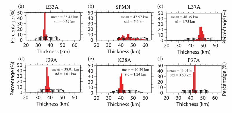
Examples of prior marginal distributions for crustal thickness at the six example stations 246
are shown as white histograms in Figure 4. The nearly uniform distribution of the prior 247
illustrates that we impose weak prior constraints on crustal thickness. 248
3.2 Joint Monte Carlo inversion and the posterior distribution 249
Once the data are prepared and the prior model space is determined, we follow Shen et al. 250
[2013b] and perform a Markov Chain Monte Carlo inversion. At each location, we 251
consider at least 100,000 trial models in which the search is guided by the Metropolis 252
algorithm. Models are accepted into the posterior distribution or rejected according to the 253
square root of the reduced χ2 value. A model m is accepted if χ(m) > χmin + 0.5, where χmin 254
is the χ value of the best fitting model. After the inversion, the misfit to the Rayleigh 255
wave dispersion curve has a χmin value less than 1 for all the stations. For receiver 256
function data, χmin is less than 1 for more than 95% of the stations. At six stations, χmin > 1 257
for the receiver functions: At two of these stations, multiple arrivals in the receiver 258
functions cannot be fit with our simple model parameterization and probably require the 259
introduction of further layers in the crust. The other four stations lie near the boundaries 260
of our study region where the receiver functions are of lower quality. 261
The principal output of the joint inversion at each station is the posterior distribution of 262
models that satisfy the receiver function and surface wave dispersion data within 263
tolerances that depend on the ability to fit the data and data uncertainties as discussed in 264
the preceding paragraph. The statistical properties of the posterior distribution quantify 265
model errors. In particular, the mean and standard deviation (interpreted as model 266
11
uncertainty) of the accepted model ensemble are computed from the posterior distribution 267
at each depth within the model. 268
Figure 4 shows posterior distributions for crustal thickness for the example stations as red 269
histograms. Compared with the prior distributions (white histograms), the posterior 270
distributions narrow significantly at five of the six stations, meaning that at these stations 271
crustal thickness is fairly tightly constrained (σ < 2 km) with a clear Moho Ps conversion 272
in the receiver function (Fig. 3a). The exception is station SPMN (Fig. 3b) in the northern 273
MCR where there is a weak Moho Ps conversion (σ > 5 km). In the six examples 274
presented in Figure 4, crustal thickness ranges from about 35 to 48 km. Over the entire 275
region of study, crustal thickness has a mean value of 44.8 km and an average 1σ 276
uncertainty of about 3.3 km. 277
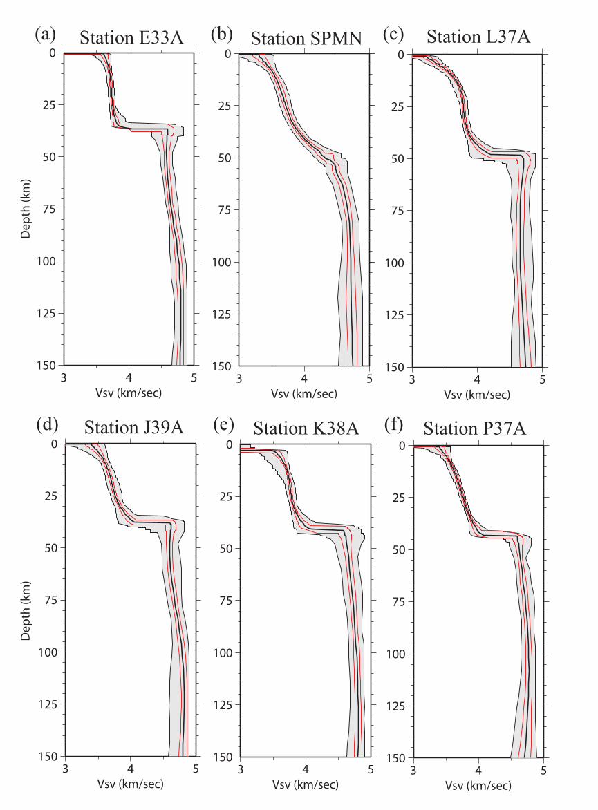
Inversion results for the six example stations are shown in Figure 5. The clear Moho with 278
small depth uncertainty at station E33A reflects the strong Moho Ps signal in the 279
back-azimuth averaged receiver function (Fig. 3a). Both the Rayleigh wave dispersion 280
and the receiver function are fit well at this station (Fig. 3a). In contrast, at station SPMN 281
(Fig. 5b) a gradient Moho appears in the model because the receiver function does not 282
have a clear Ps conversion (Fig. 3b). 283
The resulting models for the other four stations (L37A, J39A, K38A, P37A) are shown in 284
Figure 5c-f and the fit to the data is shown in Figure 3c-f. Station L37A is located near 285
the center of the southern MCR. The receiver functions computed at this station show a 286
relatively strong Moho Ps conversion at ~ 6 sec after the direct P arrival, indicating a 287
sharp Moho discontinuity at ~ 50 km depth with uncertainty of about 1.75 km. For station 288
J39A in northeastern Iowa, the clear Ps conversion at ~ 5 sec indicates a much shallower 289
Moho discontinuity at ~ 40 km with an uncertainty of about 1 km. For station K38A near 290
the eastern flank of the southern MCR, strong reverberations in the receiver function 291
indicate the existence of thick sediments but there is also a clear Moho Ps arrival. Finally, 292
a clear Moho with uncertainty less than 1 km is seen beneath station P37A in the 293
12
Mazatzal province. 294
We perform the joint inversion for all 122 TA stations in the region of study and construct 295
a mean1-D model with uncertainties for each station. We then interpolate those 1-D 296
models onto a regular 0.25°x 0.25°grid by using a simple kriging method in order to 297
construct a 3-D model for the study region [Shen et al. 2013a]. 298
Maps of the 3-D model for various model characteristics are shown in Figures 6-8. 299
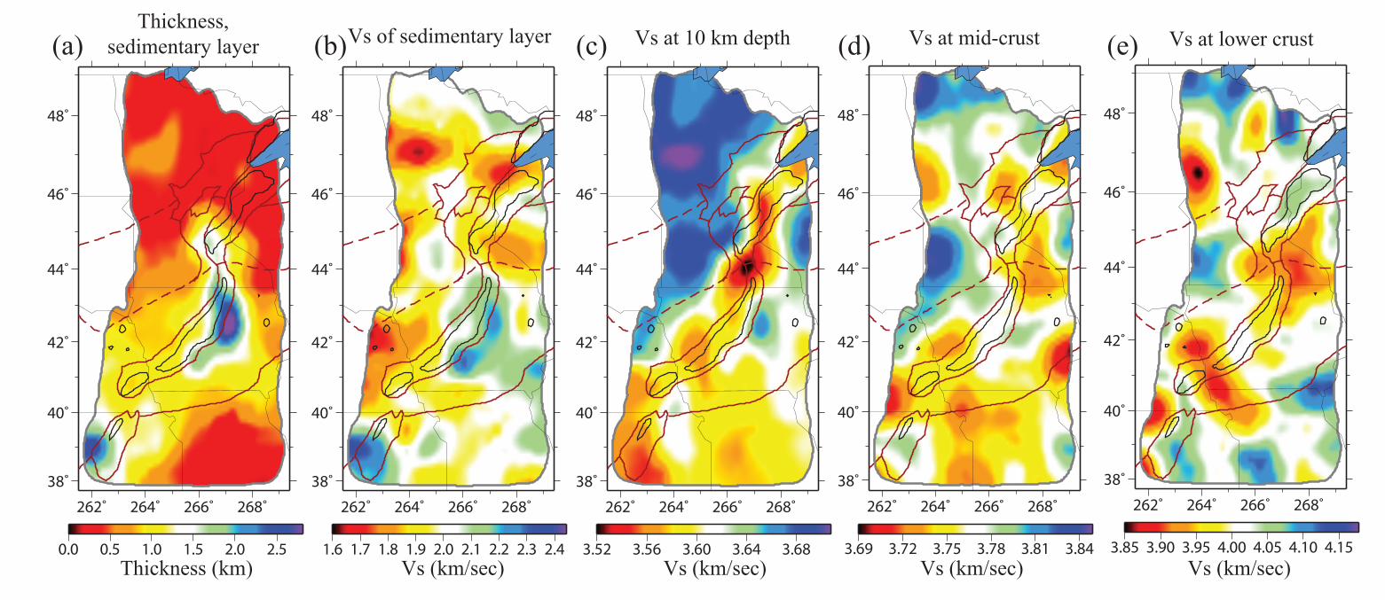
Figure 6 presents map views of the 3-D model within the crust: average thickness and Vs 300
of the sedimentary layer (Fig. 6a,b, respectively), Vs at 10 km depth (Fig. 6c), middle 301
crust defined as the average in the middle 1/3 of the crystalline crust (Fig. 6d), and lower 302
crust defined as the average from 80% to 100% of the depth to the Moho (Fig. 6e). Moho 303
depth, uncertainty in Moho depth, and the Vs contrast across the Moho (the difference 304
between Vs in uppermost mantle and lower crust) are shown in Figure 7a-c. Deeper 305
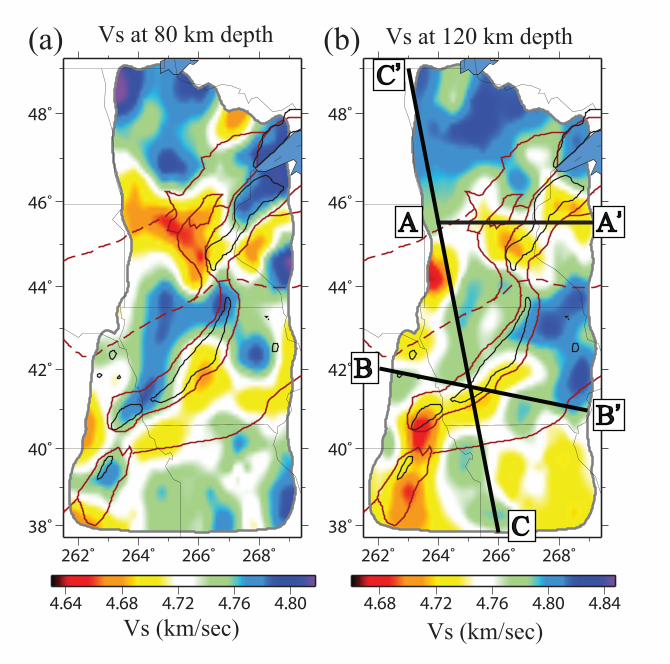
structures in the mantle are presented in Figure 8 with Vs maps at 80 km depth (Fig. 8a) 306
and 120km (Fig. 8b). Three vertical slices that cross the MCR are shown in Figure 9 307
along profiles identified as A-A’, B-B’ and C-C’ in Figure 8b. The model is discussed in 308
more detail in section 4. Although the 3-D model extends to 200 km below the surface of 309
the earth, the Vs uncertainties increase with depth below 150 km due to the lack of 310
vertical resolution. Therefore, we only discuss the top 150 km of the 3-D model. 311
4. Results and Discussion 312
4.1 Sedimentary layer 313
The sedimentary layer structure is shown in Figure 6a,b. Thick sediments (> 2 km) are 314
observed near the eastern flank of the southern MCR, thinning southward. Another thick 315
sedimentary layer appears near the southern edge of the MCR in Kansas. In the rest of the 316
area, the sediments are relatively thin (<1 km). However, because the sedimentary 317
structure is mainly inferred by receiver functions, the resulting sedimentary distribution 318
may be spatially aliased due to the high lateral resolution of the receiver functions (< 5 319
13
km) with a low spatial sampling rate at the station locations (~ 70 km). The receiver 320
functions also indicate the existence of sediments with particularly low shear wave 321
speeds in some areas. For example, strong reverberations observed in the receiver 322
function for station E33A in the first 2 sec may be fit by a Vs model with a thin (< 0.5 km) 323
but slow Vs layer (< 1.8 km/sec) near the surface (Fig. 3a). Figure 6b shows the pattern 324
of the inferred Vs in the sedimentary layer, which differs from the sedimentary thickness 325
map. Very slow sedimentary shear wave speeds are found in northern Minnesota, which 326
may be due to the moraine associated with the Wadena glacial lobe [Wright, 1962]. Some 327
of the slow sediments generate strong reverberations in the receiver functions that 328
coincide in time with the Moho signal, resulting in large uncertainties in the crustal 329
thickness map (Fig. 7b). At some other stations, sedimentary reverbarations do not 330
obscure the Moho Ps arrival; e.g., K38A (Fig. 3e). Sedimentary reverberations in the 331
receiver functions can also be seen in Figure 9 beneath the Yavapai Province in transects 332
B-B’ and C-C’, beneath the southern MCR in transect C-C’, and north of the southern 333
MCR in transect C-C’. 334
4.2 Correlations of crustal structure with the observed gravity field 335
The MCR gravity high (40 mgal anomaly outlined in the free air gravity map of Fig. 1) is 336
poorly correlated with the shear velocity anomalies presented in Figures 6-8. Because 337
positive density anomalies should correlate to positive velocity anomalies [Woollard, 338
1959], the expectation is that high velocity anomalies underlie the MCR or the crust is 339
thin along the rift. In fact, the opposite is the case. At 10 km depth, low velocity 340
anomalies run beneath the rift and, on average, the crust is thickened under the rift. Our 341
3D model does therefore not explain the gravity high that lies along the MCR. There are 342
two possible explanations for this. First, the high-density bodies that cause the gravity 343
high may be too small to be resolved with surface wave data determined from the station 344
spacing presented by the USArray. Second, small high shear wave speed bodies that 345
cause the gravity high may be obscured by sediments in and adjacent to the rift. We 346
14
believe the latter is the more likely cause of the anti-correlation between observed gravity 347
anomalies and uppermost crustal shear velocity structure beneath the rift. If this is true, 348
however, the high-density bodies that cause the gravity high would have to be in the 349
shallow crust, else they would imprint longer period maps that are less affected by 350
sediments. This is consistent with the study of Woelk and Hinze [1991] who argue that 351
the uppermost crust beneath the MCR contains both fast igneous rocks and slow clastic 352
rocks. Under this interpretation, shallow igneous rocks must dominate the gravity field 353
while the clastic rocks dominate the shear wave speeds. A shallow source for the gravity 354
anomaly is also supported by the observation that the eastern arm of the MCR, which is 355
buried under the Michigan Basin, has a much weaker gravity signature than the western 356
arm imaged in this study [Stein et al., 2011]. 357
The 3D shear velocity model is better correlated with the longer wavelengths in the 358
gravity map (Fig. 1), which displays a broad gradient across the region [von Frese et al., 359
1982]. The free-air gravity southeast of the MCR is lower (-30 mgal) than in the 360
northwestern part of the map (10-20 mgal). It has been argued that this gradient is not due 361
to variations in Precambrian structure across the sutures [Hinze et al., 1992], but may be 362
explained by a density difference in an upper crustal layer. Our results support an upper 363
crustal origin because the correlation of high shear velocities with positive long 364
wavelength gravity anomalies exists primarily at shallow depths. At 10 km depth, which 365
is in the uppermost crystalline crust (Fig. 6c), the most prominent shear velocity feature is 366
a velocity boundary that runs along the western flank of the MCR. This follows the 367
Minnesota River Valley Province-Yavapai Province boundary in the west and the 368
northeastern edge of the Craton Margin Domain in the east. North of this boundary, Vs is 369
between 3.65 and 3.7 km/sec in the southern Superior Province, while to the south it 370
decreases to between 3.5 and 3.6 km/sec in the Minnesota River Valley, Yavapai Province 371
and Mazatzal Province. This boundary lies near the contrast in free air gravity. Similar 372
features do not appear deeper in the model (Figs. 6d,e, 7). 373
15
Because receiver functions are sensitive to the discontinuity between the sediments and 374
the crystalline crustal basement, the commonly unresolved trade-off between crustal 375
structure and deeper structure in traditional surface wave inversions [e.g., Zheng et al., 376
2010; Zhou et al., 2011] has been ameliorated in the model we present here. 377
Consequently, we believe that the Vs heterogeneity present at 10 km depth in the model 378
does not arise from a vertical smearing effect in the inversion, that the high correlation of 379
Vs with the long-wavelength gravity field is confined to the upper crust, and that the 380
source of the long wavelength gravity trend is in the upper crust. 381
Additionally, there are correlations between shallow Vs structure and short wavelength 382
gravity anomalies. (1) In the gravity map, the lowest amplitudes appear near station 383
K34A on the eastern flank of the southern MCR where thick sediments are present in the 384
model (Fig. 5e). Thus, local gravity minima may be due to the presence of local 385
sediments. (2) At 10km, a very slow anomaly (< 3.5 km/sec) is observed in the gap 386
between the northern and southern MCR, which implies an upper crustal depth for the 387
discontinuity in the MCR in this area. It is not clear why such low shear wave speeds 388
appear in the upper crust here. 389
4.3 Relationship between Precambrian sutures and observed crustal structures 390
4.3.1 Great Lakes Tectonic Zone 391
In the northern part of the study region, the Great Lakes Tectonic Zone (GLTZ) suture 392
that lies between the 2.7 -2.75 Ga greenstone terrane to the north and the 3.6 Ga 393
granulite-facies granitic and mafic gneisses Minnesota River Valley sub-province to the 394
south cuts the southern end of Superior Province into two sub-provinces [Morey and 395
Sims, 1976]. The eastern part of Great Lakes Tectonic Zone in our study region is 396
covered by the Craton Margin Domain (CMD of Fig. 1), which contains several 397
structural discontinuities [Holm et al., 2007]. 398
Beneath this northernmost suture, a Vs contrast is observed in the 3-D model through the 399
16
entire crust, increasing with depth. In the upper crust (Fig. 6c), Vs is ~ 3.7 km/sec 400
beneath the Superior Province (SP) greenstone terrane and ~ 3.68 km/sec beneath the 401
Minnesota River Valley (MRV) with a relatively slow Vs belt beneath the eastern part of 402
the suture. In the middle crust (Fig. 6d), the Vs contrast is stronger. A fast anomaly (> 3.8 403
km/sec) is observed beneath the MRV itself, perhaps indicating a more mafic middle 404
crust, while in the north the SP is about 0.08 km/sec slower than the MRV. This 405
difference across the Great Lakes Tectonic Zone grows with depth to about 0.15 km/sec 406
in the lowermost crust (Fig. 6e). 407
These variations in crustal structure are also reflected in Moho depth, which is discussed 408
further in section 4.4. North of the GLTZ, a clear, large-amplitude Moho signal is seen as 409
early as 4.3 sec (Fig. 3a), although the receiver functions at some stations display large 410
reverberations from the thin slow sediments. Combined with relatively fast phase 411
velocities observed at 28 sec period in this area, the inversion yields a relatively shallow 412
Moho at about 36 km depth at station E33A and its neighboring points. To the south of 413
the GLTZ, thicker crust is found in the MRV with an average crustal thickness of about 414
46 km with a maximum thickness of about 48 km. The average uncertainties of crustal 415
thickness in the MRV are greater than 3 km suggesting that the Moho is more of a 416
gradient than a sharp boundary (Fig. 7c). A seismic reflection study in this area (Boyd 417
and Smithson, 1994) reveals localized Moho layering probably due to mafic intrusions 418
related to post-Archean crustal thickening events in this area. Our large Moho depth and 419
fast middle to lower crust (Fig. 6d,e) are consistent with this interpretation. 420
4.3.2 Spirit Lakes Tectonic Zone 421
The boundary between the Superior (SP) and the Yavapai (YP) provinces is the Spirit 422
Lakes Tectonic Zone (SLTZ), which extends east through the middle of the MCR into 423
Wisconsin. East of the MCR, the SLTZ separates the Penokean Province to the north 424
from the Yavapai Province to the south. As described in section 4.2, west of the MCR this 425
suture forms a boundary within the upper crystalline crust that correlates with the gravity 426
17
map. Structural differences between the two provinces across the suture continue into the 427
lower crust, with faster Vs in the Minnesota River Valley subprovince and slower Vs in 428
the Yavapai. In terms of Moho topography, the Yavapai Province has relatively thinner 429
crust (~ 44-45 km), becoming thinner east of the southern MCR (~ 39 km). In particular, 430
the receiver function at station J39A (Fig. 3d) displays a clear Moho Ps conversion at 431
about 4.5 sec after the direct P arrival. The resulting model for station J39A is shown in 432
Figure 4d with a crustal thickness of about 38±1.5km. This is the thinnest crust in the 433
vicinity of the rift, but is still deeper than in the Greenstone terrane in the western part of 434
the Superior Province. 435
4.3.3 Boundary between the Yavapai and Mazatzal provinces 436
The third and southernmost suture in the study region is the boundary between the 437
Yavapai (YP) and Mazatzal provinces (MP) near the Iowa-Missouri border, extending in 438
the NE-SW direction. Compared with the structural variations across the more northerly 439
sutures, the variations across this suture are subtler both in crustal velocities and crustal 440
thickness. However, lower crustal Vs is slower (< 4 km/sec) in the YP than it in the MP (> 441
4 km/sec). 442
In summary, the three major Precambrian sutures in the region are associated with crustal 443
seismic structural variations, especially across the northern (GLTZ) and middle (SLTZ) 444
sutures in the MCR region. Later cumulative metamorphism of early Proterozoic 445
accretionary tectonics [Holm et al., 2007] may have obscured structural variations across 446
the Yavapai – Mazatzal boundary. 447
4.4 Variations in crustal thickness 448
An advantage of the joint inversion of surface wave dispersion and receiver functions is 449
the amelioration of trade-offs that occur near structural discontinuities such as the base of 450
the sediments and the Moho, which hamper inversion of surface wave data alone. As 451
argued by Shen et al. [2013a,b] and many others [Bodin et al., 2012; Lebedev et al., 452
18
2013], estimates of depth to Moho as well as the velocity contrast across it are greatly 453
improved and we believe that our estimates of crustal thickness beneath the MCR are 454
reliable. 455
The map of estimated Moho topography (Fig. 7a) shows that the MCR has a deep Moho 456
(>47 km, peaking at ~50 km) in all three segments (Wisconsin/Minnesota, Iowa, 457
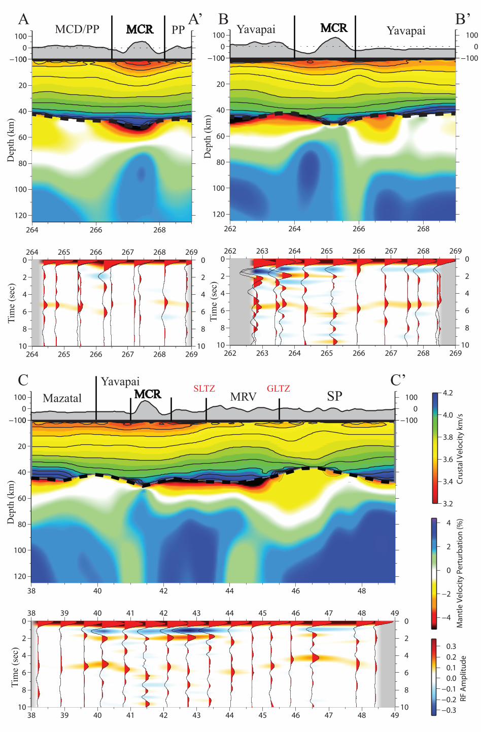
Nebraska/Kansas). The crust beneath the MCR is about 5 km thicker, on average, than 458
crustal thickness averaged across the study region. For the northern MCR, the crustal 459
thickening mostly occurs within the gravity anomaly and extends to the northeastern edge 460
of the Craton Margin Domain. In the southern MCR, crustal thickening is not uniform 461
along the rift but is most pronounced in the southern half of this segment. For the 462
Nebraska/Kansas segment, thickened crust (> 47 km) is also present, which is consistent 463
with a previous reflection study for this area [Woelk and Hinze, 1991]. 464
Uncertainties in crustal thickness for the northern segment of the MCR are larger (> 4km) 465
than for the southern segment (<2 km), as Figure 7b shows. This is because receiver 466
functions in the south display a clear P-to-S conversion associated with Moho and the 467
Moho has a larger velocity jump across it (Fig. 5c), about 0.4 km/s in the northern 468
segment and 0.55 – 0.7 km/s in the south. Between the northern and southern segments, 469
there is a shallow Moho (< 42 km) that extends eastward to the eastern Penokean Orogen 470
and perhaps further east. 471
Notable crustal thickness variations are observed in the rest of the study area as well: a 472
significantly thinned crust is seen near the western border of Minnesota within the 473
Superior Province, which changes to a thick crust with a gradient Moho at about 50 km 474
depth in the Gneiss Terrane of the Minnesota River Valley to the south. Another gradient 475
Moho is observed north of the Great Lakes Tectonic Zone in the Superior Province, 476
which is consistent with a previous reflection seismic survey in the area [Boyd and 477
Smithson, 1994]. Further south, crustal thickness lies between 42 km and 46 km in the 478
Mazatzal Province. 479
19
Three transects (identified as A-A’, B-B’, C-C’ in Fig. 8b) across the MCR are presented 480
in Figure 9. In the top panels, absolute Vs in the crust beneath the three transects is 481
shown with 0.1 km/sec contours outlined by black lines and the Moho identified by a 482
thick dashed line. In the mantle, Vs is shown as the percent perturbation relative to 4.65 483
km/sec. Transects A-A’ and B-B’ cut the northern and southern segments of the MCR, 484
respectively, and transect C-C’ cuts across the study region in the N-S direction and 485
intersects with transect B in the southern MCR. In each lower panel of Figure 9, receiver 486
function waveforms are shown for stations within a distance to each transect of 0.4°. We 487
observe in the receiver functions two major features beneath the MCR. (1) The Moho Ps 488
conversion across the northern MCR (A-A’) is obscure. (2) There is a clearer Moho Ps 489
conversion at ~6 sec for the southern MCR (B-B’ and C-C’). Thus, there is a gradient 490
Moho beneath the northern MCR, whereas there is a thick crust (>47 km) with a 491
well-defined Moho discontinuity beneath the southern MCR. As a result of the gradient 492
Moho beneath the northern MCR, crustal thickness is poorly determined (1 σ uncertainty > 493
5 km). We seek to insure that crustal thickness in the northern MCR ends up 494
approximately the same as the southern MCR. To do this, we modify the prior 495
distribution of crustal thickness to be centered on the thickness of the crust beneath the 496
southern MCR., In this way, the posterior distribution beneath the northern MCR centers 497
around 47 km, which is similar to the southern MCR.. In addition, fast lowermost crust (> 498
4 km/sec) and slow uppermost mantle (< 4.4 km/sec) result from the gradient Moho and 499
form a layer with Vs between that of normal crust and mantle. It is possible that this layer 500
results from magmatic intrusion or underplating (Furlong and Fountain, 1986). However, 501
the underplating cannot be continuous along the entire MCR, because beneath the 502
southern MCR this intermediate-velocity Vs layer is not present. In the adjacent area, 503
another gradient Moho feature is seen beneath the Minnesota River Valley, with a Moho 504
Ps conversion in the receiver functions that is weaker than those in the Superior or 505
Yavapai Provinces (transect C-C’). As discussed in section 4.3.1, this result is consistent 506
20
with a seismic reflection study in this sub-province [Boyd and Smithson, 1994] where 507
Moho layering has been inferred due to mafic intrusion in the lower crust. The other 508
features seen in these transects include the relatively thin crust (~ 40 km) near the flanks 509
of the MCR (e.g., SMCR-Yavapai boundary) and in the southern Superior Province 510
northern of the Great Lakes Tectonic Zone. The later region holds the thinnest crust 511
across the region (<38 km), and the cause of this thinning is an open question for further 512
investigation. 513
4.5 Evidence that the MCR is a compressional feature 514
Currently active rifts such as the East African Rift [e.g., Braile et al., 1994; Nyblade and 515
Brazier, 2002], Rio Grande Rift [e.g., West et al., 2004; Wilson et al., 2005; Shen et al., 516
2013a)], West Antarctic Rift [Ritzwoller et al., 2001], and Baikal rift [Thybo and Nielsen, 517
2009] as well as hot spots (e.g., Snake River Plain and Yellowstone (e.g, Shen et al., 518
2013a)) show crustal thinning. At some locations the thinned crust has been rethickened 519
by mafic crustal underplating; for example, the Baikal rift (Nielsen and Thybo, 2009) and 520
also the Lake Superior portion of the MCR [Cannon et al., 1989]. Although thermal 521
anomalies dominantly produce low Vs in the mantle underlying active rifts (e.g., Bastow 522
et al., 1998), compositional heterogeneity in the crust due to mafic underplating and 523
intrusions can overcome the thermal anomaly to produce high crustal wave speeds even 524
in currently active regions. After the thermal anomaly has equilibrated, as it has had time 525
to do beneath the MCR, high crustal wave speeds would be expected. In actuality, we 526
observe a thickened and somewhat slow crust under the MCR. We discuss here evidence 527
that the observed crustal characteristics reflect the compressional episode that followed 528
rifting [Cannon, 1994]. 529
The presence of low velocities in the upper and middle crust and crustal thickening 530
beneath the MCR has been discussed above (e.g., Figs. 6-8). Figure 9 shows transects 531
with receiver functions profiles shown for reference. Transect AA’, extending from the 532
Superior Province to the Penokean Province, illustrates that the upper crust beneath the 533
21
rift is slower than beneath surrounding areas and the crust thickens to about 50 km. In the 534
upper and middle crust, lines of constant shear wave speed bow downward beneath the 535
northern MCR, but this is not quite as clear in the southern MCR as transects B-B’ and 536
C-C’ illustrate. The gradient Moho beneath transect A-A’ appears as lower Vs in the 537
uppermost mantle in Transect A-A’. The sharper Moho beneath transects B-B’ and C-C’ 538
appears as higher Vs in the uppermost mantle. 539
These observations of a vertically thickened crust with downward bowing of upper 540
crustal velocity contours contradict expectations for a continental rift. They are, in fact, 541
more consistent with vertical downward movement of material in the crust, perhaps 542
caused by horizontal compression and pure shear thickening. Geological observations 543
and seismic reflection studies in the region also indicate a compressional episode 544
occurring after rifting along the MCR. (1) Thrust faults form a horst-like uplift of the 545
MCR, showing crustal shortening of about 20 to 35 km after rifting [Anderson, 1992; 546
Cannon and Hinze, 1992, Chandler et al., 1989; Woelk and Hinze, 1991]. (2) Uplift 547
evidence from anticlines and drag folds along reverse faults are also observed [Fox, 1988; 548
Mariano and Hinze, 1994a]. The horst-like uplift combined with reverse faults have been 549
dated to ca. 1060 Ma [Bornhorst et al. 1988; White, 1968; Canno and Hinze,1992], which 550
is about 40 Ma after the final basalt intrusion [Cannon, 1994]. (3) Seismic reflection 551
studies show a thickened crust beneath certain transects [Lake Superior: Cannon et al., 552
1989; Kansas: Woelk and Hinze, 1991]. 553
In summary, our 3-D model combined with these other lines of evidence argue that the 554
present-day MCR is a compressional feature in the crust. The compressive event 555
thickened the crust beneath the MCR and advected material downward in the crust. More 556
speculatively, rifting (ca 1.1 Ga) followed by compression may have weakened the crust, 557
which allowed for the extensive volcanism in the neighboring Craton Margin Domain 558
that appears to have occurred in response to continental accretion to the south [Holm et 559
al., 2007]. 560
22
A potential alternative to tectonic compression as a means to produce crustal thickening 561
beneath the MCR may be magmatic underplating that occurred during the extensional 562
event that created the rift [e.g., Henk et al., 1997]. Although the gradient Moho that is 563
observed beneath parts of the northern MCR may be consistent with magmatic 564
underplating, the clear Moho with the large jump in velocity across it in the southern 565
MCR is at variance with underplating. The general absence of high velocity, presumably 566
mafic, lower crust also does not favor magmatic intrusions into the lower crust. Thus, 567
although magmatic underplating cannot be ruled out to exist beneath parts of the MCR, 568
particularly in the north, it is an unlikely candidate for the unique cause of crustal 569
thickening along the entire MCR. In addition, it cannot explain the downward bowing of 570
shear wave isolines in the upper and middle crust. 571
4.6 Uppermost mantle beneath the region 572
Not surprisingly for a region that has not undergone tectonic deformation for more than 1 573
Gy, the upper mantle beneath the study region is seismically fast. The average shear wave 574
speed at 100 km depth beneath the study region is 4.76 km/s. By comparison, at the same 575
depth the upper mantle beneath the US west of 100°W is 4.39 km/s. The slowest Vs is 576
about 4.62 km/sec at 80 km depth near the border of the east-central Minnesota Batholith. 577
This is still faster than the Yangtze Craton (4.3 km/sec at 140 km depth, Zhou et al., 2012) 578
or the recently activated North China Craton (~ 4.3 km/sec at 100 km, Zheng et al., 2011), 579
but is similar to the Kaapvaal craton in South Africa (Yang et al., 2009). The rms 580
variation across the region of study is about 0.05 km/s, which is much less than the 581
variation across the western US (rms of 0.18 km/s). Thus, the variability across the 582
central US is small in comparison to more recently deformed regions. 583
Although upper mantle structural variation is relatively small across the study region, 584
Figures 8 and 9 show that prominent shear velocity anomalies are still apparent. In 585
general, the Vs structure of the uppermost mantle is less related to the location of the 586
Precambrian provinces and sutures than is crustal structure. One exception is deep in the 587
23
model (120 km, Fig. 8) where there is a prominent velocity jump across the Great Lakes 588
Tectonic Zone. The principal mantle anomalies appear as two low velocity belts. One is 589
roughly contained between the Great Lakes Tectonic Zone and the Spirit Lakes Tectonic 590
Zone, and then spreads into the Penokean Province east of the northern MCR. The other 591
extends along the southern edge of the Southern and the Nebraska/Kansas segments of 592
the MCR, particularly at depths greater than 100 km. Beneath the MCR itself, shear wave 593
speeds in the uppermost mantle are variable, although as Figure 9 illustrates there is a 594
tendency for the upper mantle beneath the MCR to be fast. The main high velocity 595
anomaly exists beneath the Superior Province with the shape varying slightly with depth. 596
This anomaly terminates at the Great Lakes Tectonic Zone, being particularly sharp at 597
120 km depth. The jump in velocity at the Great Lakes Tectonic Zone is seen clearly in 598
transect C-C’ (Fig. 9c). 599
There are three major factors that contribute to variations in isotropic shear wave speeds 600
in the uppermost mantle: temperature, the existence of partial melt or fluids, and 601
composition [Saltzer and Humphreys, 1997]. The fast average Vs in the upper mantle 602
compared with tectonic regions and recently rejuvenated lithosphere suggests no 603
existence of partial melt. Similarly, velocity anomalies in the region probably do not have 604
a tectonothermal origin because they had time to equilibrate in the last 1.1 Ga. However, 605
low velocity anomalies at greater depth may still reflect thinner lithosphere, which we 606
speculate may be the case on the southern edge of the southern MCR. Nevertheless, the 607
most likely cause of much of the variability in velocity structure in the uppermost mantle 608
is compositional heterogeneity. 609
An alternative interpretation of the relatively low Vs is a lower depletion in magnesium 610
in the mantle. Jordan [1979] argued that mantle depletion will lower density but increase 611
seismic velocities in the upper mantle. Thus, the lower wave speeds observed between 612
the Great Lakes and Spirit Lakes Tectonic Zones may be due to less depleted material 613
from the mantle rejuvenation that occurred during the rifting. Beneath the MCR near 614
24
Lake Superior area, basalts have been observed that were generated from a relatively 615
juvenile mantle source [Paces and Bell, 1989; Nicholson et al., 1997], indicating the 616
possible emplacement of less depleted material at shallower depth from the upwelling 617
during the the rifting. This possible rejuvenation process may leave an enriched mantle 618
remnant at depths greater than 100 km beneath the MCR and its surrounding (e.g., the 619
craton margin domain), causing slower Vs compared to the rest of more depleted 620
sub-cratonic lithosphere. Schutt and Lesher [2006], however, argued that mantle 621
depletion would cause relatively little change in Vs in the upper mantle. Thus, the cause 622
of the observed velocity variability in the uppermost mantle remains largely an open 623
question that deserves further concerted investigation. 624
5. Conclusion 625
Based on two years of seismic data recorded by the USArray/Transportable Array 626
stations that cover the western arm of the Mid-Continental Rift (MCR) and its 627
neighboring area, we applied ambient noise tomography using the eikonal tomography 628
method and teleseismic earthquake tomography using the Helmholtz tomography method 629
to construct Rayleigh wave phase velocity maps from 8 to 80 sec across the region. By 630
performing a joint Bayesian Monte Carlo inversion of these phase velocity measurements 631
with receiver functions, we construct posterior distributions shear wave speeds in the 632
crust and uppermost mantle from which we infer a 3D model of the region with attendant 633
uncertainties to a depth of about 150 km. This model reveals three major features of the 634
crust and uppermost mantle in this area. 635
First, the observed free air gravity field correlates with sediments and upper crustal 636
structures in three ways. (1) A thick sedimentary layer contributes to the negative gravity 637
anomalies that flank the MCR. (2) The slow upper crust at the gap between the northern 638
and southern MCR masks the high gravity anomaly that runs along the rift. (3) Shear 639
velocities in the uppermost crystalline crust are associated with a long wavelength gravity 640
anomaly that is observed across the study area. However, our 3D model does not explain 641
25
the existence of the gravity high along the rift because the crust beneath the MCR is 642
seismically slow or neutral, on average. High-density anomalies must either be smaller 643
than resolvable with our data or be obscured by sediments. We believe the latter is the 644
primary reason as the uppermost crust beneath the MCR probably contains both fast 645
igneous rocks and slow clastic rocks such that shallow igneous rocks dominate the 646
gravity field while the clastic rocks dominate the shear wave speeds. 647
Second, crustal thickening is found along the entire MCR, although along-axis variations 648
exist. Analysis of local faults and seismic reflection studies in this area provide additional 649
evidence for,a compressional inversion of the rift and crustal thickening during the 650
Grenville orogeny [French et al., 2009]. Thicker crust and a deeper Moho cause a 651
decrease in mid-crustal shear wave speeds and in Rayleigh wave phase velocities at 652
intermediate periods (15-40 sec). The uppermost mantle beneath the MCR is faster than 653
average across the study region, but velocity anomalies associated with the MCR are 654
dominantly crustal in origin. 655
Third, the seismic structure of the crust, particularly the shallow crust, displays discrete 656
jumps across the three major Precambrian sutures across the study region. This implies 657
that although the Superior Greenstone Terrane in the north collided with the Minnesota 658
River Valley more than 2 Ga ago, preexisting structural differences beneath these two 659
subprovinces are preserved. Other sutures (e.g., Spirit Lakes Tectonic Zone, 660
Yavapai/Mazatzal boundary) also represent seismic boundaries in the crust. The mantle 661
beneath the entire region is faster than for cratonic areas that have undergone significant 662
tectonothermal modification and lithospheric thinning (e.g., North China Craton), with 663
the Superior Greenstone Terrane being the least affected by events of tectonism across the 664
region. 665
In summary, the 3-D model we present here combined with other lines of evidence 666
establishes that the MCR is a compressional feature of the crust. Presumably, the closing 667
of the rift produced compressive stresses that thickened the crust beneath the MCR, 668
26
advecting material downward in the crust under pure shear. The position of the slow 669
thickened crust directly under the MCR suggests that crustal weakening during extension 670
and subsequent thickening under compression occurred as pure shear [McKenzie, 1978], 671
rather than under simple shear conditions, which would have resulted in a lateral offset 672
between surface versus deep crustal features [Wernicke, 1985]. Finally, since the MCR 673
has been inactive for long enough that thermal signals associated with tectonic activity 674
should have long decayed, our results provide a useful context for distinguishing between 675
compositional and thermal influences on seismic velocities in active continental rifts 676
[Ziegler and Cloetingh, 2004]. 677
In conclusion, we note several topics for further research. (1) For some stations, we 678
ignore intra-crustal layering, which may exist due to the thinning of the crust when rifting 679
occurred. (2) The USArray TA data do not provide ideal inter-station spacing for receiver 680
function analyses, and spatial aliasing of structures is possible. Finer sampling at select 681
areas along the rift may appreciably improve our model. (3) Our model does not reveal 682
structures deeper than about 150 km, which makes the determination of variations in 683
lithospheric thickness difficult. These issues call for further work with a denser seismic 684
array, such as the Superior Province Rifting Earthscope Experiment (SPREE) that has 685
already been installed in this area [Stein et al., 2011], as well as the input of other types of 686
geophysical data. Nevertheless, the 3-D model provides a synoptic view of the crust and 687
uppermost mantle across the region that presents an improved basis for further 688
seismic/geodynamic investigation of the MCR. 689
Acknowledgments. The facilities of the IRIS Data Management System, and specifically 690
the IRIS Data Management Center, were used to access the waveform and metadata 691
required in this study. The IRIS DMS is funded through the National Science Foundation 692
and specifically the GEO Directorate through the Instrumentation and Facilities Program 693
of the National Science Foundation under Cooperative Agreement EAR-0552316. 694
27
Aspects of this research were supported by NSF grants EAR-1053291and EAR-1252085 695
at the University of Colorado at Boulder. 696
697
698
28
Reference List 699
Bassin, C. (2000). The current limits of resolution for surface wave tomography in North 700
America. EOS Trans. AGU. 701
Bastow, I. D., Stuart, G. W., Kendall, J., & Ebinger, C. J. (2005). Upper‐mantle seismic 702
structure in a region of incipient continental breakup: northern Ethiopian 703