183
Crystallographic and Magneto-Dynamic Characterization of Thin-Film Spintronic Materials James Sizeland Doctor of Philosophy University of York Physics March 2015

Crystallographic and Magneto-Dynamic
Characterization of Thin-Film Spintronic
Materials
James Sizeland
Doctor of Philosophy
University of York
Physics
March 2015

2
Abstract
This thesis sets out to identify and characterise the critical properties of two spintronic
materials, the half-metallic Fe3O4 and the amorphous rare earth-transition metal alloy
GdFe. The critical property of Fe3O4 is its crystal ordering, due to the array of exchange
and superexchange interactions which define its conductive and magnetic behaviour. A
series of post-oxidized Fe3O4||MgO (001) thin-films have been produced and the oxide
growth has been analyzed by high resolution transmission electron microscopy
(HRTEM). The quality of the film has been assessed by magnetometry and critical
parameters for the growth of quality films are described. Previous procedures on the
(001) orientation turn out to have masked much of the disorder in the films. This meant
that judgments of quality based on magnetometry conflicted with optic data. By cutting
down the (011) plane this research was able to resolve these conflicts and effectively
explain the performance of a film as observed from magnetometry data. Previous work
has elucidated the theoretical imperfections that can exist in this material. This work
confirms the potential for these defects and has identified others. The characteristic
visibility criteria for these crystal defects are confirmed and extended. By contrast the
critical property of GdFe is the temperature dependent coupling between rare earth and
transition metal sublattices. A measurement system was constructed to resolve the
temperature dependence of the magneto-optic Kerr effect at femtosecond time scales.
By this method, the theoretical timeline of dynamic behaviour has been experimentally
validated and enhanced. Observations of resolved sublattice dynamics have been
identified and interpreted, including a clear indication of picosecond ferromagnetic
ordering. As such this work corroborates and advances existing techniques for the
production, analysis and understanding of these spintronic materials.

3
Contents
Abstract 2.
Contents 3.
List of Figures 8.
Acknowledgements 21.
Declaration 22.
1 Introduction 23.
1.1 Spintronics 23.
1.2 Origin of Magnetism 26.
1.3 Motivation 27.
1.3 Outline 29.
1.4 References 32.
2 Interpreting Magneto-Optic Dynamics in Thin-film Media 34.
2.1 Introduction 34.
2.2 Magneto-Optical Kerr Effect (MOKE) 36.
Single Detector Signal Calculations 38.
Bridge Detector Signal Calculations 39.
2.3 Ultrafast Magnetization Dynamics 41.
2.3.1 Laser-Induced Ultrafast Demagnetization 41.
2.3.2 Historical Development 45.
2.4 Laser-Induced Coherent Precession 49.
Macrospin Dynamics 49.
Effective Field 50.

4
Damping and the LLG equation 51.
Interpretation of Precessional Dynamics 53.
2.5 References 55.
3 Materials for Spintronic Applications 58.
3.1 Introduction 58.
3.2 Half-Metals: Magnetite (Fe3O4) 58.
3.2.1 Structure & Magnetic Properties 58.
3.2.3 Single Crystal Growth Considerations 62.
3.3 Rare Earth-Transition Metal Alloys: GdFe 64.
3.3.1 Structure & Magnetic Properties 64.
3.3.2 Magneto-dynamic Properties 68.
3.4 Summary 72.
3.5 References 72.
4 Quality Control of Materials 75.
4.1 Introduction 75.
4.2 Growth Techniques 75.
4.2.1 Molecular Beam Epitaxy (MBE) 75.
Growing Epitaxial Fe3O4 78.
4.2.2 Sputter Deposition 79.
4.3 Imaging Techniques 79.
4.3.1 Sample Preparation 80.
Cross-section Technique 80.
Plan-View Lift-Off Technique 83.
4.3.2 Transmission Electron Microscopy (TEM) 83.
4.3.3 Electron Diffraction 85.

5
4.3.4 Dark Field Imaging 88.
4.4 References 90.
5 Building Magnetic Characterization Techniques 91.
5.1 Introduction 91.
5.2 Measuring the Magneto-Optic Kerr Effect (MOKE) 91.
5.3 Time-Resolved MOKE Magnetometry 95.
5.3.1 Stroboscopic Techniques 95.
5.3.2 Femtosecond Laser Operation 97.
Pump Laser 98.
Seed Laser 99.
Regenerative Amplifier 100.
Maintenance 102.
5.3.3 Optics Design Process 103.
Delay Line 104.
Beam Overlap 106.
Beam conditioning 109.
5.3.4 Signal Capture & Electronic Considerations 111.
5.3.5 Design of Software 113.
5.4 References 117.
6 Materials Study of Post-Oxidized Magnetite Thin-Films 119.
6.1 Introduction 119.
6.2 Experimental 120.
6.3 Results 121.
6.3.1 Initial Investigation 121.
6.3.2 (110) Microscopy Investigation 129.

6
6.3 Fe3O4/MgO (100) APB Geometry 133.
6.3.1 Theoretical Review 133.
6.3.2 Experimental Observation 139.
6.4 Summary 142.
6.5 References 143.
7 Ultrafast Magnetization Dynamics Study of GdFe Thin-Films
144.
7.1 Introduction 144.
7.2 Methodology 145.
7.3 Results 146.
7.3.1 Static Hysteresis Measurements 146.
7.3.2 Pump Fluence Series of Gd0.25Fe0.75 148.
Reflectivity 148.
Ultrafast Demagnetization 150.
Magnetization Recovery Time 155.
Magnetic Precessional Frequency 162.
Magnetic Precession Damping 169.
7.3 Summary 171.
7.3.1 Evidence for Magnetization Compensation
Temperature 171.
7.3.2 Evidence for Angular Momentum Compensation
Temperature 173.
7.4 References 174.
8 Conclusions & Further Work 175.
8.1 Discussion of Post-Oxidized Fe3O4 175.
7
8.1.2 Further Research 176.
8.2 Fluence Dependent Magneto-Dynamics in GdFe 177.
8.2.1 Discussion of Results 177.
8.2.2 Further Research 179.
8.3 Concluding Remarks 180.
8.4 References 180.
Glossary 181.

8
List of Figures
Figure 1.1: Venn diagram of the three particle interactions which encompass the
field of spintronics. 24.
Figure 1.2: Moore’s law of exponential improvement in technology showing year on
year growth in data storage density in magnetic media. 25.
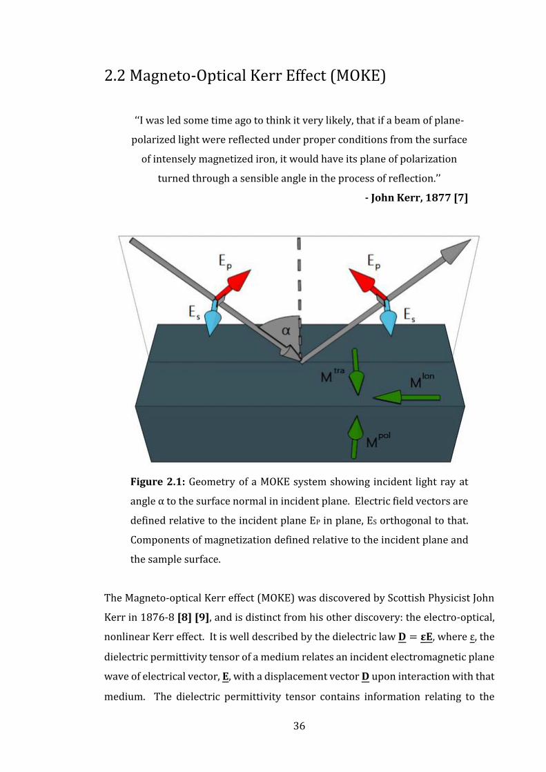
Figure 2.1: Geometry of a MOKE system showing incident light ray at angle αto the
surface normal in incident plane. Electric field vectors are defined relative to the
incident plane EP in plane, ES orthogonal to that. Components of magnetization
defined relative to the incident plane and the sample surface. 36.
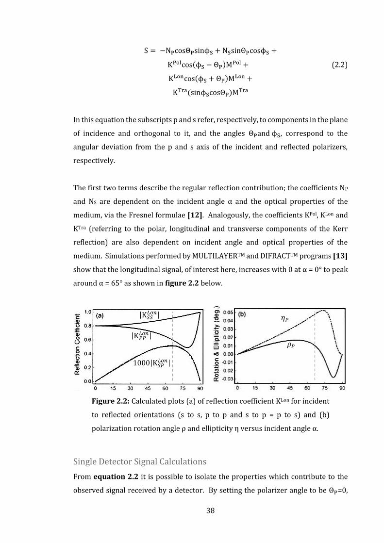
Figure 2.2: Calculated plots (a) of reflection coefficient KLon for incident to reflected
orientations (s to s, p to p and s to p = p to s) and (b) polarization rotation angle ρ
and ellipticity η versus incident angle α. 38.
Figure 2.3: Graph of signals for a single detector scheme. Normalized signal
observed for a theoretical isotropically magnetized sample, showing the relative
signal amplitude of each Kerr orientation as a function of analyzer angle for incident
s and p polarized light source. Signal maximized for 90° angle between polarizer
and analyzer. 39.
Figure 2.4: Graph of signals for a two detector scheme. Normalized signal observed
for a theoretical isotropically magnetized sample, showing the relative signal
amplitude of each Kerr orientation as a function of analyzer angle for incident s and
p polarized light source. Signal maximized for 45° angle between polarizer and
analyzer. 40.
Figure 2.5: Three thermodynamic reservoirs in a ferromagnetic metal. Each can be
initially excited by different mechanisms (e.g. photon injection, magnetic field

9
change, mechanical stress). This is followed by a relaxation to the other reservoirs
dependent on the strength of coupling between each. 41.
Figure 2.6: Time-energy correlation graph, plotting t = h/E. This gives a direct
comparison between frequency, time and associated energies. General ranges of
interactions are marked. 43.
Figure 2.7: Graphs showing spin (Ts), electron (Te) and lattice (Tl) temperatures
from specific heat calculations on Ni (left) and pump-probe SHG measurements over
fluence series 250-1150 µJ/cm2 also on Ni (right). 46.
Figure 2.8: (a) Time-resolved spin polarization of photo-emitted electrons for Ni
films; (b) induced ellipticity (open circles) compared to induced rotation (filled
circles) showing a phase shift between them; (c) Polar Kerr hysteresis of CoPt3 alloy
at pump delays, showing transient M-H loop evolution. 48.
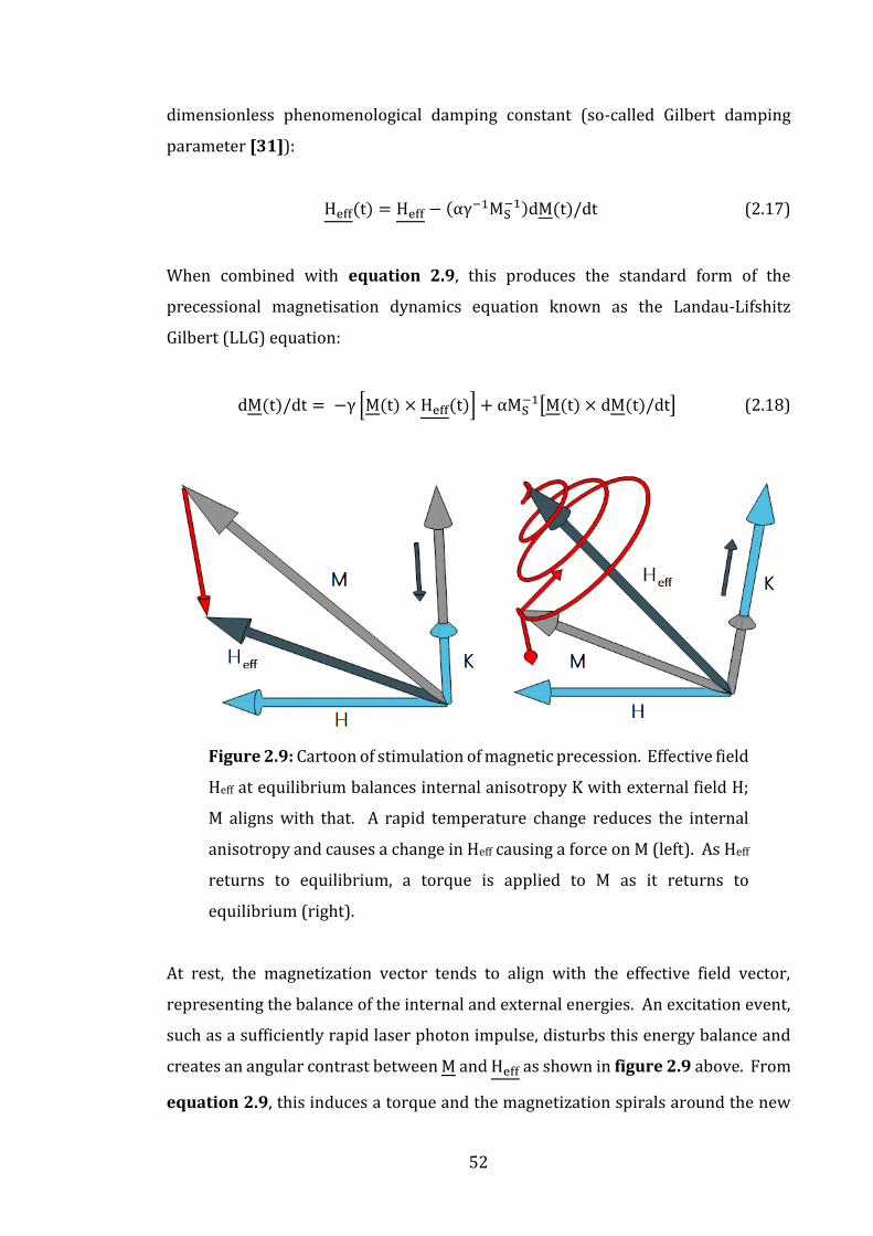
Figure 2.9: Cartoon of stimulation of magnetic precession. Effective field Heff at
equilibrium balances internal anisotropy K with external field H; M aligns with that.
A rapid temperature change reduces the internal anisotropy and causes a change in
Heff causing a force on M (left). As Heff returns to equilibrium, a torque is applied to
M as it returns to equilibrium (right). 52.
Figure 2.10: Plot of damped sinusoidal oscillation equation showing ideal
exponential decay envelope from A to M0. 54.
Figure 3.1: Illustrations of the three most common orientations of the Fe3O4 cubic
inverse spinel crystal unit cell. The structure is comprised of a fcc O2+ lattice ((O),
red atoms), equal numbers of Fe3+ and Fe2+ ions filling half of the octahedral site
((B), dark blue atoms) and Fe3+ ions filling ⅛ of the tetrahedral sites ((A), light blue
atoms). These orientations provide different visibility of atomic columns. 59.
Figure 3.2: Cartoons of interatomic interactions which exist in crystalline magnetite
(left) and example positions of superexchange interactions within the magnetite

10
unit cell (right), displaying (i) ~90 weakly ferromagnetic superexchange interaction
on B sites, (ii) ferromagnetic double exchange interaction on B sites, and (iii)
strongly antiferromagnetic superexchange interaction between octahedral and
tetrahedral iron sites. 60.
Figure 3.3: Cartoon of (a) Fe3O4 (001) unit cell, containing octahedral (dark blue)
and tetrahedral (light blue) iron ions, showing superexchange bonds via oxygen
(red) sublattice. By comparison, to scale (b) MgO (001) unit cell, containing
magnesium (yellow) sublattice bonded to oxygen (red) sublattice. 63.
Figure 3.4: Schematic illustration of APB types with shift vectors (left) showing
translational and rotational shifts used to calculate TEM visibility conditions and
220 type TEM dark field images of APBs in Fe3O4/MgO (001) films of (a) 6nm, (b)
12nm, (c) 25nm and (d) 50nm thickness (right). 64.
Figure 3.5: Hartree-Fock theoretically calculated radial influence of Gd electron
orbitals. The 4f orbital, which carries the magnetic moment, is shielded deep within
the ion, affected by the environment only via intra-atomic exchange with the 5p
orbital. 65.
Figure 3.6: Schematic guide to the temperature dependence of both individual
sublattices along with their combined effect on the net magnetic characteristics of
the material. Shows the two compensation temperatures, magnetic (TM) and
angular momentum (TA) along with the Curie temperature (TC) these broadly
describe the temperature dependent characteristics of a RE-TM material. 67.
Figure 3.7: Schematic demonstration of the energy transfer channels which exist
within a RE-TM alloy under laser photon stimulation. 70.
Figure 3.8: (a) Theoretical calculated response rates for Gd5d, Fe3d and Gd4f
electron orbitals under pulsed laser stimulation. (b) Cartoon schematics of the two
observable modes of spin precession, the FMR coherent mode and the high
temperature exchange mode. (c) Experimental observations of temperature and
11
angular momentum compensation in GdFeCo as well as the observed Gilbert
damping. 71.
Figure 4.1: Schematic of MBE system. Sample is positioned at the top of the
chamber behind a mechanical shutter. An electron source gun is guided onto a
sublimation source in a Hearth, which ejects a molecular beam towards the sample.
Various pumps and heat sinks are used to maintain the low pressure environment.
A plasma oxygen source is fitted here to introduce molecular oxygen into the
chamber for post-oxidation experiments. 77.
Figure 4.2: Iron oxide phase diagram, showing the spectrum of oxides which can be
formed under various temperature and oxygen environmental conditions. Pure
Fe3O4 (magnetite) exists under a very narrow range between ~900-1500° and
~27.5-28.5% oxygen composition by weight. 78.
Figure 4.3: Example images of several stages of polishing a cross-section sample,
showing the quality of the interface required for a successful sample. 81.
Figure 4.4: Cartoon schematic of the arrangement of materials combined to make a
cross section TEM sample. Slices of a sample are glued face to face (film surfaces
together) and backed by Si supports. After thinning one side, a Cu grid is glued to
support the sample once it reaches <50 µm thick. 81.
Figure 4.5: After PIPS milling, the sample is considered ready when a clear band of
rainbow fringes are observable at the interface. This is due to the thickness of that
region being of the scale order of the wavelength of visible light. 82.
Figure 4.6: Schematic showing ray diagram of a standard Transmission Electron
Microscope (TEM) setup. Showing the series of lenses which collect and shape the
electron beam created at the top of the column. 84.
Figure 4.7: Calculated diffraction pattern for Fe3O4 (001) showing the Miller index
for each spot corresponding to a plane in the real-lattice. 86.

12
Figure 4.8: Examples of basic Miller indices for a simple cubic system. 87.
Figure 4.9: Schematic of planar defect geometry used in Howie-Whelan
approximation. 88.
Figure 5.1: Schematics showing Kerr rotation of polarization causing a linear
increase in the intensity component along the analyzer axis (left) and a simple cross-
analyzer detector configuration (right). 93.
Figure 5.2: (a) Design of bridge detector built and used in this investigation showing
two trans-impedance photodiode amplification circuits mounted to a rotating frame
to detect orthogonal polarization components. Only 400 nm probe light is admitted
and the frame is able to rotate around the axis of the probe beam to balance the
detectors. The setup allows easy access to variable capacitors to tune the temporal
response of each diode independently. (b) A schematic circuit diagram for the trans-
impedance circuit built. 94.
Figure 5.3: Difference between bridge detector photodiode 1 and 2 on oscilloscope.
Shows an example of a signal spike observed if the detector timings are mismatched.
This is adjusted for by changing the detector amplifier capacitance. 95.
Figure 5.4: Historical image of frame by frame observation of a horse in motion by
Eadweard Muybridge showing early example of observation of a dynamic event
captured faster than real time. 96.
Figure 5.5: Schematic showing the combination of laser instruments to form the
high-power, short-rise pulsed laser essential to this investigation. 97.
Figure 5.6: The seed pulse is stretched, reducing its peak power, before
amplification and then recompressed to form a short, high power pulse. This allows
greater amplification circumventing the power damage threshold of the amplifier.
101.

13
Figure 5.7: Amplifier regeneration profile observed on oscilloscope. Just the input
Pockels cell activated (left) and the output Pockels additionally activated (right).
This shows an example of a well-tuned regeneration, points of note: low background
interference, sharp build-up, output timing set to output high pulse power.
101.
Figure 5.8: Example of effect of laser stability noise on the detector output shown
on oscilloscope for an unstable situation (left) and after optimizing (right). Showing
signal from detector 1 (top trace), inverted signal from detector 2 (bottom trace)
and the optimized difference between the channels (middle trace). 102.
Figure 5.9: Schematic of the ultimate experimental set-up used in this investigation.
The laser output is split into transmitted pump (92%) and reflected probe (8%) by
a beam-splitter. The pump beam (red) passes through a delay line, optical chopper
and beam reducer before being focused onto the sample. The probe (blue) passes
through a BBO wavelength doubling crystal and a polarizer before being focused
onto the sample. 104.
Figure 5.10: Alignment of the delay line. A pinhole is mounted on the delay line
during alignment to measure the relative deviation in the beam. A one axis
translation stage and rotation mount are used to adjust the beam entering the delay
line to minimize this deviation. 105.
Figure 5.11: Frame by frame camera capture of the pump beam spot on the sample
during a delay line movement using two mirrors. Shows a non-linear drift as the
delay line is moved from one end to the other. This is caused by sub-micron
unevenness in the delay line tilting the mirrors. 106.
Figure 5.12: Schematic of alignment of the three interdependent lenses required to
focus the laser and then obtain a true image of the sample surface. 107.
14
Figure 5.13: Camera images of alignment of the three interdependent lenses
required to observe the sample surface clearly. The image lens is added and moved
to focus (left); the reflected lens is added and moved until a wide-field image of the
sample surface is in focus (middle); the incident lens is added and moved until the
beam focus is observed again. This is done for both pump and probe together and
overlapped (right). 108.
Figure 5.14: Ray diagram of geometry for approximating beam focus diameter
based on lens focal length, f, and incoming beam divergence, θd1 from a collimated
beam. 110.
Figure 5.15: Ray diagram of geometry for calculating change in beam radius and
divergence from a collimated beam. 110.
Figure 5.16: LabVIEW software front panel, designed to show a number of useful
values such as the applied field strength and runtime information. 114.
Figure 5.17: LabVIEW software settings menu, designed to allow a large amount of
control over the experimental settings. Delay line steps are set up here in ranges to
allow the time sensitivity to be varied based on the scale of dynamics in each range
(middle). A field sweep can also, optionally, be set-up for at each delay step (right).
115.
Figure 5.18: Image showing LabVIEW main experiment ‘For loop’. 116.
Figure 5.19: LabVIEW software pre-run information. Each run is saved with a data
sheet containing the useful experimental information and save filenames and
folders are then procedurally generated. 117.
Figure 6.1: VSM measurements for three post-oxidized samples. Sample A (green)
shows an over oxidized state; sample B (red) shows a more favourable square Fe3O4
response; sample C (blue) shows an iron dominated signal for a thicker film with a
limited oxidation depth. 121.

15
Figure 6.2: Table showing growth and magnetometry information for thin over-
oxidized sample A; thin less oxidized sample B; thick unoxidized layer-dominated
sample C. 122.
Figure 6.3: HRTEM cross-section of 15 minutes oxidation time (top) and 60 minutes
oxidation time thin samples (bottom). Showing the substrate, film and vacuum
(guide lines have been added to compare with figure 6.5). 123.
Figure 6.4: Select area diffraction of 15 minute oxidation time thin-film (top left);
60 minute oxidation time thin-film (top middle); MgO substrate (top right);
calculated pattern of Fe3O4 (001) (bottom left) and MgO (001) (bottom right).
Yellow squares mark out common oxygen sublattice pattern and blue squares mark
out Fe3O4 unit cell pattern, displaying inverse spinel structure. 124.
Figure 6.5: Bragg filtered images of (a) 60 minute oxidation time thin-film and
substrate; (b) 15 minute oxidation time thin-film and substrate. Greater disorder is
observable in (a) compared to (b). 125.
Figure 6.6: TEM image showing long range film with sharp interface and uniform
depth (left). Select area diffraction (right) shows Fe3O4 (100), Fe (110) and MgO
(100) crystalline order epitaxially stacked. 126.
Figure 6.7: HRTEM images of Fe3O4 (100)||Fe (110) interface (far left) with Bragg
filtered image (mid left) and of Fe (110)||MgO (100) interface (mid right) with
corresponding Bragg filtered image (far right). Crystal plane dislocations are
identified from the Bragg filtered images and circled showing regular predictable
mismatch in Fe3O4||Fe, but irregular mismatch in Fe||MgO. 127.
Figure 6.8: Illustrations of the three most common orientations in the Fe3O4 cubic
inverse spinel crystal unit cell. The (110) direction resolves each atomic column
independently, unlike the other two. 128.

16
Figure 6.9: (110) direction HRTEM of (a) 9 minutes post-oxidized sample, showing
Fe (100), Fe3O4 (110) and substrate. Interface transition takes place over ~5
monolayers. 129.
Figure 6.10: (110) direction HRTEM of (b) 27 minutes, (c) 45 minutes post-oxidized
sample, showing Fe (100), Fe3O4 (110) and substrate. Interface transition in (b)
much sharper than figure 6.9 (a) and (c). 130.
Figure 6.11: Bragg filtered images of 9 minutes (left) and 45 minutes (right)
samples. Shows increase in disorder with oxidation time more clearly than figure
6.5. 131.
Figure 6.12: Example line contrast profiles of 9 (left) 27 (middle) and 45 (right)
minute sample images. These are used to determine the thickness of each film with
a rigorous measure. 132.
Figure 6.13: Example of two geometric shifts of the Fe3O4 unit cell on the (grey-
scale) MgO (100) lattice. They may appear to be unique, but are in fact mirror
images. 134.
Figure 6.14: Schematic showing proposed terminating planes of Fe3O4 (100) unit
cell. Four octahedral (B) iron atoms exist in each plane, notably the oxygen lattice is
constant through each plane. 135.
Figure 6.15: In-plane APBs on Fe3O4 (100). 136.
Figure 6.16: 1⁄2 z-shift out-of-plane APBs on Fe3O4 (100). 136.
Figure 6.17: 1⁄4 z-shift out-of-plane APBs on Fe3O4 (100). 137.
Figure 6.18: 3⁄4 z-shift out-of-plane APBs on Fe3O4 (100). 137.

17
Figure 6.19: Non-integer unit cell shifts and visibility criteria, showing the in-plane
shifts (grey) and out-of-plane shifts. 138.
Figure 6.20: Images showing example diffraction pattern for 15mins sample (top
left); a TEM image of the sample surface (top right); calculated gamma-phase Fe2O3
maghemite, observed in plan-view analysis (bottom left) and calculated Fe3O4
diffraction pattern (bottom right). 139.
Figure 6.21: Images showing plane-view TEM images of two regions of 15 minute
post-oxidized film under [220] dark field conditions which show a large defect
density. 140.
Figure 6.22: Images showing plane-view TEM images of 15 minute post-oxidized
film under [400] dark field conditions, showing visible defects, as well as Moiré
fringes. 141.
Figure 7.1: Normalized static MOKE longitudinal hysteresis measurements
showing the anisotropic magneto-optic response. All TRMOKE measurements are
undertaken at the in-plane hard axis, 0° here. 147.
Figure 7.2: Amplitude of maximum reflectivity peak (red) compared to equivalent
maximum Kerr signal peak (blue) as a function of pump fluence. Reflectivity shows
a discontinuity between 37-42 µJ/cm2 which is not seen in the Kerr signal data. Both
curves show a possible gradual saturation at higher fluences. 149.
Figure 7.3: Recovery time constant of the local sample reflectivity, as a function of
pump fluence. Two regimes of energy dissipation are observed. For low fluence,
this is not energy dependent, but for higher fluence it becomes significantly so.
149.
Figure 7.4: Graph showing ultrafast demagnetization curves for low (a), (black), (23
µJ/cm2) and high fluence (b), (red), (76 µJ/cm2). Inset graph shows the picosecond

18
timescale drop in magnetization and the high frequency artefacts which affect the
regime highlighted in the blue dashed region. 151.
Figure 7.5: Ultrafast moment flipping contrast, defined in figure 7.4, shows the
strength of the ferromagnetic state as the Gd and Fe moments align for a picosecond
above a critical thermal threshold, corresponding to TMcomp. 152.
Figure 7.6: Schematic timeline of the ultrafast magnetic reversal behaviour.
154.
Figure 7.7: Time for Gd sublattice to reach internal equilibrium, showing 2 critical
temperature points (a) and (b) 154.
Figure 7.8: TRMOKE rotation signal as a function of pump fluence for low pump
powers. Oscillatory recovery is observed for each, with the first oscillation being
gradually absorbed into the long range recovery curve. 155.
Figure 7.9: TRMOKE rotation signal as a function of pump fluence for high pump
powers. Oscillatory recovery is all but obscured by the long range recovery curve.
156.
Figure 7.10: Graph showing an example magnetization recovery time curve for low
pump fluence (25 µJ/cm2), with fitted exponential decay; recovery is rapid and
strongly oscillatory. 158.
Figure 7.11: Graph showing an example magnetization recovery time curve for high
pump fluence (82 µJ/cm2), with fitted exponential decay; recovery is much slower
and oscillatory behaviour is both suppressed and delayed. 159.
Figure 7.12: Graph showing time constant τ as a function of pump fluence (black),
showing the recovery time from each maximum demagnetization state; and total
recovery time (blue), which includes the time from the initial pump event, showing
the total time associated with elevated energy in the spin reservoir. 160.

19
Figure 7.13: Comparison of energy dissipation from spin reservoir (black), (Kerr
signal) and lattice reservoir (red, dominant temperature reservoir over long
timescale represented in Reflectivity signal). 161.
Figure 7.14: Schematic showing energy and angular momentum gain and loss
channels. Spin lattice relaxation is dependent on the dominant moment’s spin-orbit
coupling, which is Gd at low temperatures, and swaps to Fe above TMcomp.
162.
Figure 7.15: Example of magnetic precession residual, after removing recovery
slope low fluence measurement (black) (25 µJ/cm2), with fitted sinusoidal decay
(red). 164.
Figure 7.16: Example of magnetic precession residual, after removing recovery
slope low fluence measurement (black) (82 µJ/cm2), with fitted sinusoidal decay
(red). 164.
Figure 7.17: Residual for 65 µJ/cm2 fluence plot. This shows the two frequencies,
separated by a temperature boundary. 165.
Figure 7.18: FFT series, showing the gradual growth of lower frequency precession
while the dominant frequency begins to fall, followed by the rapid reversal of the
frequency dominance, and finally the lower frequency drops again at the highest
laser pump fluences. 166.
Figure 7.19: Comparison of FFT frequency vs curve fitted frequency for coherent
precession regime. Shows slow increase with fluence followed by a significant drop
off after 71 µJ/cm2, lower frequency oscillation observed at higher temperature
becomes stronger at higher fluences. 167.

20
Figure 7.20: Graph showing resonance amplitudes from FFT as a function of pump
fluence for both oscillation frequencies observed. This shows swapping of dominant
precessional mode after TMcomp which is also then quenched at TAcomp. 167.
Figure 7.21: Graphs showing examples of cropped FMR mode precession data with
damped sinusoidal fitting. 169.
Figure 7.22: Graph showing Gilbert damping parameter as a function of fluence.
Highlighted are the magnetization TMcomp and angular momentum TAcomp
compensation temperatures. 170.
Figure 8.1: Dynamic hysteresis measurements taken at 0.5 ps intervals after pump
event 179.

21
Acknowledgements
It has been a long and educational journey that leads up to the submission of this
document. A task that would not have been possible without the support and
guidance of so many people at the University of York and beyond. I’d like to take
this opportunity to acknowledge Professor Kevin O’Grady for introducing me to the
world of research, without this inspiration I would not be where I am today. To my
supervisors Dr. Vlado Lazarov and especially Dr. Jing Wu, have opened up new
worlds for me. To Professor Rex Godby and Dr Stuart Cavill for your advice and
counsel.
I’d like to thank the support staff, particularly Bob Hide, Dave Coulthard, Neil
Johnson and Mark Laughton for their guidance and friendship throughout this
process. To the students who went before me, from whom I have learned a great
deal, Dr. James Naughton, Dr. Andy Vick, and Dr. Tuyuan Chen. And to my fellow
students, too numerous to list, who have shared in the triumphs and frustrations
which we all faced.
Finally to my family, thank you for supporting me this far.
For Rod.

22
Declaration
The research present here in this doctoral thesis is the work of the author, James
Sizeland, except where explicitly acknowledged or referenced in the text, in
accordance with the examination regulations of the University of York. This work
has not previously been presented for an award at this, or any other, University.

23
Chapter 1
Introduction
1.1 Spintronics
Spintronics is an umbrella term for the area of condensed matter physics which
deals with the understanding of the electron spin in conjunction with its charge and
their interaction with photons, all three of which represent information carriers [1].
The major motivations in this area are twofold; enhancement of modern cutting-
edge electronics technology and greater appreciation of the fundamental physical
principles which inevitably emerge when pushing the limits of both size and speed
of functional devices. The name is derived from a portmanteau of spin and
electronics.

24
Figure 1.1: Venn diagram of the three particle interactions which
encompass the field of spintronics. [2]
It is an area covering a large number of specialisms (as shown in figure 1.1),
covering topics from quantum computing [3] and graphene nanostructures [4] to
year on year improvements in speed and scale of the technology in our pockets and
homes [5]. By necessity it is a fast moving and rapidly advancing field, fuelled by its
eminently applicable nature, producing many exciting developments over a
relatively short span of time. The field received a Nobel Prize in Physics in Albert
Fert and Peter Grünberg in 2007 for their work on giant magnetoresistance (GMR)
[6] [7]. Magnetoresistance is employed in a spin-valve structure in the read-heads
of the hard disk drives (HDD), found in most personal computers for the last 30
years. It is used to convert the magnetic field of a data bit to an electronic signal.
Such information is stored in magnetic bits, where anisotropy limits the
magnetization to one of two orientations, read in binary by allocating them as ones
or zeroes. The discovery of GMR, and subsequent adoption of materials supporting
it, has increased magnetoresistance conversion efficiencies from ~10% to >40% [8]
allowing even smaller magnetic bits to be used. This is fuelling the growth in areal
data density as predicted by Moore’s Law (figure 1.2).

25
Figure 1.2: Moore’s law of exponential improvement in technology
showing year on year growth in data storage density in magnetic media.
[2]
Future efforts are focused on greater improvements in GMR devices, but
additionally on technologies such as magnetic random access memory (MRAM)
which aim to replace both current HDD and conventional RAM architecture as a
“universal memory”, offering non-volatility, nanosecond read and write times,
competitive density and significant savings in both power and real estate, crucial in
mobile devices. That being said, there are equally important fundamental physics
questions at stake. Questions like the fundamental timescales of spin coherence.
Fundamentally, spin is a quantum-mechanical effect whose interaction with charge
and other such phenomena offer invaluable information on matter.
26
1.2 Origin of Magnetism
Extensive descriptions of magnetism exist in many places and this section will serve
to introduce a few of the key points which will be relevant throughout this work. [9]
[10].
Two main theoretical approaches exist to apply quantum theory to magnetism,
these being the localized model and the band model. The first describes a system
dominated by intra-atomic electron-electron interactions, which define atomic
moments. Interatomic interactions are small and compete with thermal energy to
define magnetic behaviour. The second considers magnetic carriers as itinerant
(mobile), heavily influenced by interatomic interactions and forming electron
energy bands. Intra-atomic interactions produce ordered magnetic states based on
the proportions of electron spins oriented up and down. A spectrum of behaviour
exists between these two extremes and both are necessary to fully characterize a
range of magnetic material properties. For instance, transition metals, such as iron
(Fe) are well described by the band model, whereas rare earths, such as Gadolinium
(Gd) require a combined approach.
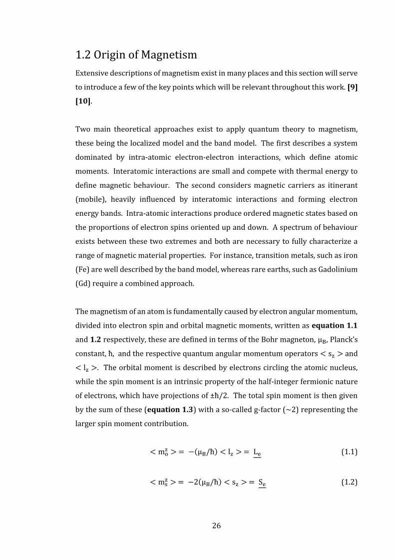
The magnetism of an atom is fundamentally caused by electron angular momentum,
divided into electron spin and orbital magnetic moments, written as equation 1.1
and 1.2 respectively, these are defined in terms of the Bohr magneton, μB, Planck’s
constant, ħ, and the respective quantum angular momentum operators < sz > and
< lz >. The orbital moment is described by electrons circling the atomic nucleus,
while the spin moment is an intrinsic property of the half-integer fermionic nature
of electrons, which have projections of ±ħ/2. The total spin moment is then given
by the sum of these (equation 1.3) with a so-called g-factor (~2) representing the
larger spin moment contribution.
< moz > = −(μB/ħ) < lz > = Le (1.1)
< msz > = −2(μB/ħ) < sz > = Se (1.2)
27
M = Le + gSe (1.3)
While conservation of energy is an important factor in all physical processes,
modern treatments of magnetism are focused on conservation of angular
momentum, which requires the magnitude and vector of Le and Seto remain
constant unless angular momentum is transferred between them or away to the
environment. From here it becomes necessary to mention the three magnetic inter-
and intra-atomic interactions which define the magnetic character of a material:
1. The exchange interaction defines a material’s spin moment and is a
consequence of interatomic electron-electron coulomb interaction.
Electrons of neighbouring atoms align parallel (ferromagnetic) or
antiparallel (antiferromagnetic), depending on the material dependent sign
of the exchange integral Jex.
2. The spin-orbit interaction describes the coupling strength between
Le and Se. It is on the order of 10 − 100 × smaller than the exchange
interaction for transition metal 3d electron orbitals, but notably larger for
rare earth 4f electron orbitals. It also determines the magneto-crystalline
anisotropy of a solid material.
3. The Zeeman interaction describes the coupling between a material’s total
magnetic moment and an externally applied magnetic field.
1.3 Motivation
Both of the materials studied in this project, half-metallic Fe3O4 (magnetite) and the
rare earth-transition metal alloy GdFe represent important aspects of spintronic
research [11] [12]. Each material contains its own set of unique challenges and
opportunities, from an engineering perspective and equally from a theoretical and
experimental scientific perspective.

28
Magnetite is an abundant, naturally occurring cubic crystal oxide of iron. It is
magnetic at room temperature and was thought to have been discovered by the
inhabitants of the Magnesia region of ancient Greece, from which the material and
the magnetism itself took their names [13]. The complex interactions of the atoms
within this structure give rise to both ferromagnetic and antiferromagnetic
components, due to super-exchange interactions. This results in a net ferrimagnetic
material with a relatively high Curie temperature (Tc) of ~860K making it stable
within the running parameters of all but the most extreme electronic devices.
Magnetite is also an electrical conductor and displays half-metallic properties to the
extent that it is theorised to be a 100% spin polarisable material [14]. These
properties make it a very promising material for application in modern spintronic
devices such as spin-valves, characteristically requiring thin-films of a few hundred
of nanometres at most [15].
The necessity for pure single crystal growth throws up a range of new challenges, as
at this length scale, the well understood bulk behaviour begins to break down, and
interfacial effects begin to become much more dominant. So far however such
attempts to integrate this material have provided limited success, hindered by low
magnetoresistance observations in thin-film prototypes [16]. As the magnetic
character of Fe3O4 is defined by its crystal structure, these limitations have been
attributed to the existence of a large number of crystal defects possible within its
epitaxial film. Such defects, known as antiphase domain boundaries (APBs) disrupt
the population of superexchange interactions. These APBs are locations where the
repeating pattern of the crystal structure is interrupted, introducing random
interatomic coupling. Advances in molecular beam epitaxy (MBE) deposition
techniques as well as more detailed work on the structure and formation process of
this material are working to resolve these issues. As such it is important to gather
an understanding of the nature and density of defects present within the film, as
these will provide a fundamental limit on the efficiency of any spintronic devices.
By contrast GdFe belongs to a group of materials which exist as amorphous alloys,
whose magnetic characteristics have been shown to be robustly independent of
their microstructure [17]. The rare-earth transition metals exist as ferrimagnetic

29
thin-films with two semi-independent magnetic moments, coming from separate
electron orbitals. These sublattices critically have very different temperature
responses, and exhibit compensation temperatures, at which the barrier to magnetic
reversal becomes very large and any stored magnetic information is extremely
shielded from unwanted thermal disorder. In order to manipulate the magnetic
information then, rapid control of the temperature of the material is needed; to raise
it to an unstable state, induce a magnetic reversal and return to rest stability. It has
been shown [18] [19] that this barrier to reversal can be overcome on a sub
nanosecond timescale by inducing a coherent magnetic precession (ferromagnetic
resonance) and more recently [20] [21] investigations have reported on
mechanisms for even faster reversal via sub picosecond optical excitation from a
laser pulse. Laser induced magnetisation reversal investigations are well placed to
provide further information on these still poorly understood [22] mechanisms.
The key motivations for this investigation were to better understand the critical
parameters which affect the magnetic character of these two materials in thin-film.
This was achieved by developing and commission a measurement apparatus for
spatial and temporally resolved magnetic measurements used to understand
temperature dependence of the magnetic behaviour of GdFe as well as investigating
techniques to understand the effects of growth and structure on Fe3O4.
1.3 Outline
In this thesis, two different methodological techniques of investigating the magnetic
character of thin-film media are discussed. These techniques are divided into self-
contained chapters based on themes of materials science and magneto-optics.
Within this division, each chapter is designed to be as self-contained as possible,
which results in some limited restatement of key facts with referential pointers to
other sections for greater detail.
Chapter 2: This describes the theoretical background required to understand the
magneto-optic work investigated in this thesis. $2.2 Introduces the concept of the
Magneto-optic Kerr effect (MOKE) and provides a quantitative discussion of the

30
geometry and analysis of such measurements. $2.3 develops this discussion for the
case of ultrafast (<100 ps) optically induced demagnetization and provides a
historical contextualization for the technique. Following this, the longer timescale
recovery process is discussed in detail in $2.4, including the energy and angular
momentum considerations and the Landau-Lifshitz Gilbert (LLG) equation which
describes such behaviour.
Chapter 3: Here the theoretical material considerations are presented. $3.2
discusses the nature of magnetite, including its crystallographic qualities and quirks.
This presents the necessary framework required for growth and structure
investigations of this material, in the context of its magnetic behaviour. $3.3 then
discusses the key properties of GdFe and their physical origins. The unique
magnetic properties of rare-earth transition metals thin-films are also provided in
more detail here.
Chapter 4: Provides the growth and structural characterization techniques required
to control the quality of thin-film growth. While this project has not been focused
growth method, but rather post-growth characterization, the methods of growth
encountered in this investigation are introduced in $4.2 to provide context for the
later work. $4.3 then provides details of the experimental and theoretical
techniques which were used and developed during the course of this investigation
to obtain and analyze high resolution electron microscopy images. This work, along
with the results provided in chapter 6 formed the first year and a half of my degree.
Chapter 5: $5.2 provides a background for the detection of the magneto-optic Kerr
effect and is provided as a stand-alone technique discussion, or as a supplementary
document to the theoretical discussion in chapter 2. $5.3 details the method and
understanding required to construct a high powered femtosecond time-resolved
MOKE apparatus. This laser system was obtained and commissioned as part of this
investigation as was the optical setup and data acquisition programmes also
detailed here.

31
Chapter 6: A critical high resolution transmission electron microscopy (HRTEM)
investigation into the quality of magnetite thin-films produced by post-oxidation of
epitaxially grown iron films. This investigation begins in $6.3 with cross-sectional
HRTEM of 3nm films under varied oxidation times which show very clear
differences in the quality of magnetic ordering and the corresponding hallmarks in
the material structure. $6.4 then provides a theoretical discussion of allowed ABP
defects and their observation criteria in dark field imaging, followed by an
experimental observation from plan-view HRTEM imaging.
Chapter 7: Details a magneto-optical investigation of a critical composition ratio
GdFe thin-film. It provides a systematic series of measurements in pulsed laser
pump energy density (fluence) to identify the critical energy transfer mechanisms
taking place on a picosecond timescale. It identifies key temperatures and
characteristics of the material and provides an important collection of information
with which to feedback to the further growth and optimization of such materials.
Chapter 8: Summarises the key points and provides a discussion of further work
which would benefit from this research.
32
1.4 References
[1] S. A. Wolf, et al., Magn. and Mat., 294, 1488 (2001)
[2] A. Hirohata and K. Takanashi, J. Phys. D: Appl. Phys., 47, 193001 (2014)
[3] T. D. Ladd, et al., Nature 464, 45 (2010)
[4] W. Han, et al., Nature Nanotechnology, 9, 794 (2014)
[5] S. A Wolf, Proceedings of IEEE, 98, 2155 (2010)
[6] P. A. Grunberg, Rev. Mod. Phys., 80, 1531 (2007)
[7] A. Fert, et al., J Magn. Magn. Mat., 140-144, 1 (1995)
[8] M. N. Baibich, et al., Phys. Rev. Lett., 61, 2472 (1988)
[9] F. Gautier and M. Cyrot, Magnetism of Metals and Alloys (North-Holland
Publishing Company, 1982)
[10] J. Stӧhr and H. C Siegmann, Magnetism: from Fundamentals to Nanoscale
Dynamics (Springer Verlag, Berlin, 2006)
[11] T. Hauet, et al., Phys. Rev. B, 76, 144423 (2007)
[12] D. Venkateshvaran, et al., Phys. Rev. B, 79, 134405 (2009)
[13] F. D. Stacey and S. K. Banerjee, The Physical Principles of Rock Magnetism
(Elsevier Science, 2012)
[14] S. M. Thompson, et al. J. Appl. Phys., 107, 09B102 (2010)

33
[15] D. Tripathy, et al., Phys. Rev. B, 75, 012403 (2007)
[16] J-B Moussy, J. Phys. D: Appl. Phys., 46, 143001 (2013)
[17] S. Mangin, et al., Nature Mat., 13, 286 (2014)
[18]C. H. Back, et al., Phys. Rev. Lett., 81, 3251 (1998)
[19] T. Gerrits, et al., Nature (London), 429, 850 (2002)
[20] K. Vahaplar, et al., Phys. Rev. Lett. 103, 117201 (2009)
[21] I. Radu, et al., Nature (London) 472, 205 (2011)
[22] V. López-Flores, et al., Phys. Rev. B, 87, 214412 (2013)

34
Chapter 2
Interpreting Magneto-Optic Dynamics in Thin-film Media
2.1 Introduction
Linearly polarized light, incident on a material exhibiting a net magnetization will
undergo an ordinary metallic interaction causing an ellipticity in any reflected and
transmitted components [1]. Alongside this ellipticity, there will be a rotational
effect proportional to the net magnetization; this is known as a magneto-optic effect.
When referring to the transmitted light, this is known as the Faraday Effect and is
proportional to the magnetization in the direction of light propagation. In reflection,
the effect is known as the magneto-optic Kerr effect (MOKE). Both the Faraday
Effect and MOKE are first-order effects, linear with magnetization, and are described
by circular birefringence, whereby left- and right-handed polarizations propagate at
different speeds and are selectively absorbed. As linearly polarized light can be
considered a superposition of equal left- and right-handed polarizations, the effects
can cause the shape and angle of plane-polarized light incident on such a medium to
be modified [2] [3]. Second-order magneto-optic effects, such as the Voigt effect,
also exist, which are quadratic with magnetization and produced by second-order
linear magnetic birefringence. These effects are only a factor at normal incidence,
when net magnetization is applied in the plane perpendicular to the incident light,

35
and will not be treated further here. As the rotation is proportional to the
propagation length through the material, the Faraday Effect was historically easier
to detect than MOKE, despite being limited by the necessity for transmission
through the medium, where MOKE only requires a reflective surface. For a long time
the Kerr effect was considered to be ‘rather weak and difficult’ [1] to obtain
meaningful information from until background subtraction methods were
improved.
The timescales of changes in magnetization, in response to external stimuli, can vary
greatly from millions of years in geography, to decades in magnetic storage devices,
to nanoseconds in magnetic hard drive read and writing, and further still.
Composition, structure and scale of constituent parts play a key role in defining each
of these time regimes. Particularly of interest to Spintronics research are three
methods of manipulating magnetic ordering on a sub-microscale, namely pulsed
field, spin current and pulsed laser stimulation [4]. Of these, pulsed laser is the only
method able to reach the sub picosecond timescale.
Over the past 20-30 years, the development of pulsed lasers has allowed science and
technology to push further into faster and faster magneto-dynamics, down to the
timescales of fundamental physical processes [5] [6]. The so-called ultrafast regime
loosely refers to the timescales below 100 ps, the intrinsic spin-lattice relaxation
time, defined by the time-energy correlation. The questions of the fundamental
limits of these processes are still as relevant today and with fundamental limits to
magnetic pulse technology being reached, alternative sources of magnetization
manipulation are all the more relevant in pushing speed limits.
This chapter discusses the current understanding and required knowledge to
perform and appreciate magneto-optic characterization experiments, particularly
time-resolved, pump-probe Kerr effect magnetometry. It goes into detail on the
development of pulsed laser induced dynamics.
36
2.2 Magneto-Optical Kerr Effect (MOKE)
‘‘I was led some time ago to think it very likely, that if a beam of plane-
polarized light were reflected under proper conditions from the surface
of intensely magnetized iron, it would have its plane of polarization
turned through a sensible angle in the process of reflection.’’
- John Kerr, 1877 [7]
Figure 2.1: Geometry of a MOKE system showing incident light ray at
angle α to the surface normal in incident plane. Electric field vectors are
defined relative to the incident plane EP in plane, ES orthogonal to that.
Components of magnetization defined relative to the incident plane and
the sample surface.
The Magneto-optical Kerr effect (MOKE) was discovered by Scottish Physicist John
Kerr in 1876-8 [8] [9], and is distinct from his other discovery: the electro-optical,
nonlinear Kerr effect. It is well described by the dielectric law 𝐃 = 𝛆𝐄, where ε, the
dielectric permittivity tensor of a medium relates an incident electromagnetic plane
wave of electrical vector, 𝐄, with a displacement vector 𝐃 upon interaction with that
medium. The dielectric permittivity tensor contains information relating to the

37
magnetization vector of the interacted medium and material specific constants [10]
[11]. It can be expanded to give the following:
D = ε(E + iQM × E) (2.1)
In equation 2.1, ε is the dielectric permittivity constant, M is the magnetization
vector of the medium and Q refers to the (material dependent) maximum strength
of the Kerr effect, which is roughly proportional to Ms, the saturation magnetization
of the medium (or sublattice). The cross product relationship between Mand E
describes a Lorentz force, υL = −M × E, and shows the symmetry of the
polarization displacement, with respect to E.
The geometry of a MOKE system is defined relative to the sample surface normal
and the incident plane made by the incident and reflected beam; the axis of
polarization is referred to as p in the plane of incidence, and s perpendicular to it
(see figure 2.1). The effect is separated into three distinct orientations; the first of
these is referred to as longitudinal MOKE, (MLon) and is due to the magnetization
component in-plane with the material surface and parallel to the plane of reflection
[1]. A linearly polarized light source incident on the material will cause an
oscillation of the electrons in the plane of the material surface and parallel to the
polarization vector E. This regularly reflected light, N, will remain polarized parallel
to E. Additionally, due to the Lorentz force υL, a small electron oscillation will be
induced in-plane with the material surface and perpendicular to E, causing a fraction
of the light to be polarized perpendicular to E upon reflection. This fraction is
referred to as the Kerr amplitude, K, and together with N, causes the rotational effect
on the reflected polarization vector, proportional to |M|. The other two MOKE
orientations are known as polar (MPol) and transverse (MTra), and refer to the
magnetization vector out-of-plane with the material surface, and in-plane but
orthogonal to the incident light plane, respectively. Combining the three
orientations, relative (to the incident) signal amplitude can be quantified as follows
in equation 2.2.
38
S = −NPcosΘPsinϕS + NSsinΘPcosϕS +
KPolcos(ϕS − ΘP)MPol + (2.2)
KLoncos(ϕS + ΘP)MLon +
KTra(sinϕScosΘP)MTra
In this equation the subscripts p and s refer, respectively, to components in the plane
of incidence and orthogonal to it, and the angles ΘPand ϕS, correspond to the
angular deviation from the p and s axis of the incident and reflected polarizers,
respectively.
The first two terms describe the regular reflection contribution; the coefficients NP
and NS are dependent on the incident angle α and the optical properties of the
medium, via the Fresnel formulae [12]. Analogously, the coefficients KPol, KLon and
KTra (referring to the polar, longitudinal and transverse components of the Kerr
reflection) are also dependent on incident angle and optical properties of the
medium. Simulations performed by MULTILAYERTM and DIFRACTTM programs [13]
show that the longitudinal signal, of interest here, increases with 0 at α = 0° to peak
around α = 65° as shown in figure 2.2 below.
Figure 2.2: Calculated plots (a) of reflection coefficient KLon for incident
to reflected orientations (s to s, p to p and s to p = p to s) and (b)
polarization rotation angle ρ and ellipticity η versus incident angle α.
Single Detector Signal Calculations
From equation 2.2 it is possible to isolate the properties which contribute to the
observed signal received by a detector. By setting the polarizer angle to be ΘP=0,
|K𝑆𝑆𝐿𝑜𝑛|
|K𝑃𝑃𝐿𝑜𝑛|
1000|K𝑆𝑃𝐿𝑜𝑛|
𝜂𝑃
𝜌𝑃

39
the signal becomes a function of the analyzer angle,ϕS as shown in equation 2.3
below. Figure 2.3 shows the angular variation in the components of this signal for
the incident p-polarized (ΘP=0) and s-polarized (ΘP = π/2) for an isotropically
magnetized sample.
S = −NPsinϕS + KPolcos(ϕS)MPol + (2.3)
KLoncos(ϕS)MLon + KTra(sinϕS)MTra
It can be seen that the largest longitudinal and polar signals are received when the
analyzer is oriented at 90° to the polarizer angle. This is known as a cross-polarizer,
or cross-analyzer arrangement. The regular reflected signal is also minimized at this
orientation.
Figure 2.3: Graph of signals for a single detector scheme. Normalized
signal observed for a theoretical isotropically magnetized sample,
showing the relative signal amplitude of each Kerr orientation as a
function of analyzer angle for incident s and p polarized light source.
Signal maximized for 90° angle between polarizer and analyzer.
Bridge Detector Signal Calculations
For dynamic measurements involving small signals and requiring reflectivity
information, a configuration of two detectors can be introduced to collect all light

40
reflected from a sample, divided into two orthogonal components. This scheme is
known as a bridge detector and is arranged with a reference state such that the
reflected light intensity is equally split into the two detectors by a rotating polarizing
beam splitter (see chapter 5 for further details on measurement technique).
Following equation 2.2 for a single detector and setting the total signal, STotal =
SA(ϕs) + SB(ϕs), where the angle between SA(ϕs) and SB(ϕs) is fixed to be 90°,
equivalent graphs can be produced for this arrangement (see figure 2.4).
Figure 2.4: Graph of signals for a two detector scheme. Normalized
signal observed for a theoretical isotropically magnetized sample,
showing the relative signal amplitude of each Kerr orientation as a
function of analyzer angle for incident s and p polarized light source.
Signal maximized for 45° angle between polarizer and analyzer.
The longitudinal and polar signals are maximized at 45° to the polarizer angle, which
is the point at which the two detectors will be balanced. Again the regular reflection
is minimized at the same point, but only in the p-polarized incident orientation. For
s-orientation, the regular reflection is maximized inverse to the longitudinal signal.
It is for this reason that p-polarized incident configuration has been used for all
MOKE measurements in this investigation.
At set-up the analyser angle ϕs is then fixed at +45° for SA and -45° for SB ready to
detect variations in ϕp caused by changes in the magnetization state of the sample.
41
The Kerr signal is then found from the difference between detectors: SKerr =
SA(ϕp) − SB(ϕp). This leads to a voltage output which is linear with Kerr rotation
(with the small angle approximation), with an offset signal S0.
SKerr ≈ S0ϕp
2.3 Ultrafast Magnetization Dynamics
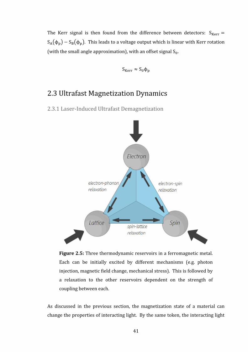
2.3.1 Laser-Induced Ultrafast Demagnetization
Figure 2.5: Three thermodynamic reservoirs in a ferromagnetic metal.
Each can be initially excited by different mechanisms (e.g. photon
injection, magnetic field change, mechanical stress). This is followed by
a relaxation to the other reservoirs dependent on the strength of
coupling between each.
As discussed in the previous section, the magnetization state of a material can
change the properties of interacting light. By the same token, the interacting light

42
can also affect the magnetization state of the material in return. The absorption of
light by a magnetic material is described by energy transfer and angular momentum
transfer [5]. This has a direct and indirect effect on its magnetization state, with
timescales dominated by that interaction and interplay between three
thermodynamic reservoirs, electron, lattice and spin (figure 2.5).
The initial interaction between a light source and a metallic system occurs by
transfer of energy from photons to the degenerate electron gas creating electron-
hole pairs which rapidly thermalize by means of electron-electron interactions [14].
The electron reservoir temperature increases extremely (typically >1 kK) and
rapidly, due to a low heat capacity, and creates a non-equilibrium with the lattice
reservoir. Energy transfer to the lattice via phonons then rapidly cools the electron
reservoir and raises the temperature of the lattice reservoir before propagating and
dissipating. Thermal equilibrium is reached between the electron gas and lattice
within ~1 ps. The specific heat of the lattice is much higher than that of the electron
gas, and as such the temperature rise of the lattice is significantly lower. Initial
photon energy absorption is well described by the Beer-Lambert law:
T =I(d)
I0= exp[−α(ω)d] (2.4)
This equation relates the transmission of light, T, through a material to the angular
frequency dependent optical absorption coefficient α(ω) and the path length
through that material, d. The absorption coefficient can be further expressed as:
α(ω) =4πk
λ (2.5)
It is then related to the wavelength of the incident light, λ, and the imaginary
component of the material’s complex refractive index, k. The penetration depth,
1/α(ω), for visible light sources (1.5-3 eV) incident on metallic surfaces varies
linearly with λ from around 10-30 nm. This depth must be taken into consideration
when analysing results from thin-film media, as the effect of any oxide layer or dis-
uniformity of the material with depth will be much greater.
43
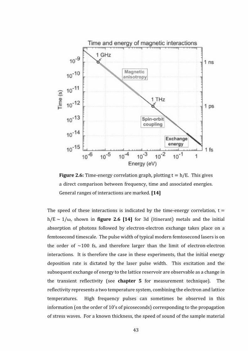
Figure 2.6: Time-energy correlation graph, plotting t = h/E. This gives
a direct comparison between frequency, time and associated energies.
General ranges of interactions are marked. [14]
The speed of these interactions is indicated by the time-energy correlation, t =
h/E ∼ 1/ω, shown in figure 2.6 [14] for 3d (itinerant) metals and the initial
absorption of photons followed by electron-electron exchange takes place on a
femtosecond timescale. The pulse width of typical modern femtosecond lasers is on
the order of ~100 fs, and therefore larger than the limit of electron-electron
interactions. It is therefore the case in these experiments, that the initial energy
deposition rate is dictated by the laser pulse width. This excitation and the
subsequent exchange of energy to the lattice reservoir are observable as a change in
the transient reflectivity (see chapter 5 for measurement technique). The
reflectivity represents a two temperature system, combining the electron and lattice
temperatures. High frequency pulses can sometimes be observed in this
information (on the order of 10’s of picoseconds) corresponding to the propagation
of stress waves. For a known thickness, the speed of sound of the sample material

44
can be calculated from the round trip time. Energy transfer is constrained by the
(material dependent) strength of electron-phonon coupling, defined by the degrees
of freedom of scattered electrons and those at the Fermi surface.
Crucially for the investigation of magneto-dynamics, is the existence and influence
of spin ordering. After the initial photon-electron interaction, the electron reservoir
is in general raised to temperatures above the Curie temperature, TC. Energy is
dispersed by electron-phonon coupling to the lattice system, but also to the spin
system. This transfer can either be by rapid direct electron-spin coupling or by
much slower spin-lattice coupling and it is pertinent to ask:
● How quickly can energy transfer into and out of the spin reservoir take place
and how quickly can the spontaneous magnetization respond to such a
transfer?
In order to approach this question, it is useful to consider the conservation of
angular momentum, which can be expressed by the Hamiltonian:
J = Le + Se + Lp + Lω (2.6)
ΔLe + ΔSe + ΔLp + ΔLω = 0 (2.7)
These equations relate the total angular momentum to the orbital momentum of the
electron system, Le, the total electron spin momentum, Se, the lattice angular
momentum, Lp, and that of the excitation photons, Lω. The local system can be
considered closed on the sub-picosecond timescale.
It has been argued [15] that ΔLP in the above equation 2.7 might be too slow to be
included as in general spin-lattice interactions are considered to occur on the ~100
ps timescale. ΔLω is agreed to be negligible due to the degree of circular polarization
contributed by the photons being small. The remaining major components belong
to the electron system, Je = Le + Se, and as the total magnetic moment can defined
as M = Le + gSe (where g ≈ 2) this implies that magnetic dynamics are caused by a

45
redistribution of electron orbital and spin angular momentum. In 3d transition
metals at rest, Se >> Le; transfer from Se → Le would cause an increase, rather than
a decrease, in magneto-optic (MO) response with laser heating, which has not been
reported. As a result, some fast contribution from coherent phonon spin-lattice
exchange cannot be neglected entirely and must be considered. This also highlights
how important the conservation of angular momentum is to any dynamic magnetic
process.
In order to manipulate the spin system both the transfer of energy and angular
momentum must be involved. Due to the tighter restrictions on angular momentum
exchange therefore the above questions can be reframed as:
● How quickly can angular momentum be exchanged to and from the spin
system and from which reservoirs is this most dominant?
In order to approach this question however, one must also ask:
● How quickly and how precisely can we measure magneto-dynamics at this
extreme timescale?
2.3.2 Historical Development
The experimental study of ultrafast magneto-dynamics began with relatively simple
metallic systems, such as Fe and Ni, and developed alongside the evolution of short-
pulse lasers. The photon energy of a laser pulse can be used to ‘pump’ energy into a
magnetic medium, causing both thermal and non-thermal effects. Early
experiments [16-19] were restricted by the limitations of pulsed lasers which, at 60
ps - 10 ns, were on the timescale or slower than the spin-lattice relaxation of the
systems they wished to explore.

46
Figure 2.7: Graphs showing spin (Ts), electron (Te) and lattice (Tl)
temperatures by [20] from specific heat calculations on Ni (a) and pump-
probe SHG measurements over fluence series 250-1150 µJ/cm2 by [21],
also on Ni (b).
It was not until 1996, (Beaurepaire et al. [20]) that experimental observations were
possible in which the laser pulse fall-off was sharp enough that the system
relaxation did not simply follow the excitation curve of the laser pulse and instead
reached non-equilibrium conditions. Beaurepaire et al. used a 60 fs pulsed laser to
observe MOKE of 22nm Ni thin-films (see figure 2.7), due to it having the lowest TC
of the transition metals. The work observed an electron thermalization time of
~260 fs by measuring the transient reflectivity and calculated an electron
temperature decay of around 1 ps, while observing a maximum spin temperature
(from hysteresis) only within 2 ps, supporting the case for separate spin and
electron reservoirs. Following on from this work, Hohlfeld et al. [21] reported a

47
year later on pump-probe second harmonic generation, also on Ni thin-films, with a
150 fs pulsed laser. This work corroborated the electron thermalization time of
Beaurepaire et al., but additionally observed that beyond ~300 fs electron and spin
reservoirs had equilibrated such that local magnetization was governed by the
electron temperature. They also showed the first series of pump fluence
measurements on this timescale, showing that a classical M(T) graph could be
reproduced even before electron-lattice thermal equilibrium has been reached.
Critically both studies indicated magnetization change faster than spin-lattice
relaxation time. In the same year Scholl et al., [22] using 170 fs pump-probe two-
photon photoemission, reported observation of two separate demagnetization
processes. Attributed to electron-electron “Stoner excitations” and spin-lattice
(phonon-magnon) scattering, these were ~300 fs and >500 ps respectively and
stated that the electron system is ‘inextricably coupled’ to the local spin moment for
itinerant ferromagnets. Despite numerous attempts, this separation has not been
reproduced and the true origin of the observation remains ambiguous.
Following this collection of early papers, a sceptical treatment of the experimental
findings was developed by, notably, Koopmans et al. [23]. This work on Cu/Ni/Cu
wedges challenged the previous assumption that a direct relationship exists
between sample magnetization and measured magneto-optic response. Koopmans
demonstrated, by polar time-resolved (TR)MOKE, an optically induced non-
magnetic component in the initial Kerr response. They showed that during the first
500 fs, a delay between the evolution of Kerr ellipticity and Kerr rotation existed,
which also showed no external applied field dependence. It was concluded that
while ultrafast dynamics does occur, reported observations of <100 fs (e.g.
Aeschliman et al. [24]) after photon injection were unlikely to be magnetically
derived, though contested by Wilks et al. [25] This detachment between true
magnetization dynamics and observed magneto-optics was further corroborated by
ab initio calculations in Ni by Oppeneer and Liebsch [26] who showed that the
conductivity tensor, and thus the complex Kerr angle, can be significantly distorted
under a non-equilibrium electron distribution. These papers concluded that due to
state-blocking effects, magneto-optic observations before the first picosecond
cannot be reliably interpreted as representing the true magnetization.
48
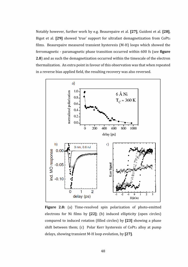
Notably however, further work by e.g. Beaurepaire et al. [27], Guidoni et al. [28],
Bigot et al. [29] showed ‘true’ support for ultrafast demagnetization from CoPt3
films. Beaurepaire measured transient hysteresis (M-H) loops which showed the
ferromagnetic - paramagnetic phase transition occurred within 600 fs (see figure
2.8) and as such the demagnetization occurred within the timescale of the electron
thermalization. An extra point in favour of this observation was that when repeated
in a reverse bias applied field, the resulting recovery was also reversed.
Figure 2.8: (a) Time-resolved spin polarization of photo-emitted
electrons for Ni films by [22]; (b) induced ellipticity (open circles)
compared to induced rotation (filled circles) by [23] showing a phase
shift between them; (c) Polar Kerr hysteresis of CoPt3 alloy at pump
delays, showing transient M-H loop evolution, by [27].

49
Due to the complexity of the processes involved, the exact origin of ultrafast
magneto-dynamics remains uncertain. What is known is that laser-induced
ultrafast demagnetization (with a sufficiently short laser pulse) can occur on a sub
300 fs timescale and that this is brought about by the exchange between three
thermal reservoirs through electron-spin and lattice-spin interactions.
2.4 Laser-Induced Coherent Precession
Over a picosecond time-scale, thermal equilibrium between the electrons and lattice
is reached, but the lattice temperature remains elevated in relation to the
environment and most likely the local magnetization is out of equilibrium. In this
regime, within a small volume, spin contributions can be considered as a coherent
macrospin, due to the tight binding effect of the exchange interaction. In this regime
a coherent magnetic precession, known as a ferromagnetic resonance (FMR), can
occur. Phenomenologically this is described by the Landau-Lifshitz Gilbert (LLG)
equation [30]. Time-resolved measurements of this precession can provide
quantitative information regarding the anisotropy, switching and damping
characteristics of a given magnetic material.
Macrospin Dynamics
The process dictating the path back to magnetic equilibrium can be treated semi-
classically starting generally with Newton’s second law of motion, relating angular
momentum L(t) to the torque τ(t) (equation 2.8). Specifically in the case of a
magnetic material this torque is caused by an angular difference between M(t) and
Heff as shown in equation 2.9:
dL(t)/dt = τ(t) (2.8)
dM(t)/dt = −γ [M(t) × Heff] (2.9)
γ = 2πgμB/h (2.10)
50
ω = γHext (2.11)
Here, M(t) is the summation of the magnetic dipole moments of the individual spins
within a ferro- (or ferri-) magnetic system and Heff, is the total effective magnetic
field. γ is the gyromagnetic ratio (equation 2.10), which relates the local system
magnetic moment to its angular momentum and is quantum mechanical in nature.
In this equation, g is the spectroscopic splitting Lande factor, μB the Bohr magneton
and h, Planck’s constant.
These equations lead to a precessional dynamic motion of M(t) around Heff at an
angular frequency, ω, determined by that effective field and the gyromagnetic ratio
(equation 2.11). As an order of magnitude estimate, for a free electron spin, γ ≈
2π(28) GHz/T, which gives a precessional period of ~360 ps (frequency of 2.8 GHz)
in a 0.1 T (1 kOe) external field.
Effective Field
The effective magnetic field vector Heff represents the minimization of the
competing energy terms associated with the local system. This energy is generally
considered to be made up of contributions from four sources: Zeeman energy EZee,
exchange energy Eex, (magnetocrystalline) anisotropy energy Eani and
demagnetizing energy Edem in the form:
Heff = −(1/ μ0)[∂(Eeff)/ ∂M] (2.12)
The Zeeman energy (equation 2.13) is the interaction between the magnetization,
M and the external field, Happ, and is minimized when they are aligned.
EZee = −μ0 ∫ M ⋅ HappdVV
(2.13)
The exchange energy (equation 2.14) comes from the interatomic quantum
mechanical exchange interaction due to electron charge distributions, discussed in

51
more detail in chapter 3. It is generally minimized by uniform spatial distribution
of the magnetization and proportional to the exchange constant, A. This term is only
applied in the case of larger areas, where spatial variation is more important.
Eex = A ∫ (|∇Mx|2 + |∇My|2
+ |∇Mz|2) (1/MS2)dV
V (2.14)
The anisotropy energy (equation 2.15) comes from the spin-orbit interaction,
producing directional energy variation based on the crystal geometry of the
material. It is minimized by the magnetization aligning along an easy axis and is
proportional to the anisotropy constant, K and a geometry dependent anisotropy
field, HK.
Eani = K ∫ (M ⋅ HK)2
(1/MS2)dV
V (2.15)
The demagnetizing energy (equation 2.16) is the effect of the magnetic fields
created by the magnetization itself. This acts to minimize the total magnetic energy,
by forming closed loops of magnetization and attempting to inhibit flux leakage and
is heavily dependent on the macroscopic shape of the sample.
Edem = −( μ0/2) ∫ M ⋅ HdemdVV
(2.16)
The equilibrium state of the total effective field direction is a balance between the
external applied field Happ and the internal fields.
Damping and the LLG equation
In addition to the precessional frequency, an energy dissipation channel (viscous
damping term) must be introduced to avoid the unphysical case of perpetual motion.
This causes the magnetization, over time, to come to rest aligned with the effective
field. In its simplest form, this is done by assuming that the damping is linear and
isotropic and achieved by including an extra time varying dissipation term to the
effective field with an expression in the form of equation 2.17 in which α is the
52
dimensionless phenomenological damping constant (so-called Gilbert damping
parameter [31]):
Heff(t) = Heff − (αγ−1MS−1)dM(t)/dt (2.17)
When combined with equation 2.9, this produces the standard form of the
precessional magnetisation dynamics equation known as the Landau-Lifshitz
Gilbert (LLG) equation:
dM(t)/dt = −γ [M(t) × Heff(t)] + αMS−1[M(t) × dM(t)/dt] (2.18)
Figure 2.9: Cartoon of stimulation of magnetic precession. Effective field
Heff at equilibrium balances internal anisotropy K with external field H;
M aligns with that. A rapid temperature change reduces the internal
anisotropy and causes a change in Heff causing a force on M (left). As Heff
returns to equilibrium, a torque is applied to M as it returns to
equilibrium (right).
At rest, the magnetization vector tends to align with the effective field vector,
representing the balance of the internal and external energies. An excitation event,
such as a sufficiently rapid laser photon impulse, disturbs this energy balance and
creates an angular contrast between M and Heff as shown in figure 2.9 above. From
equation 2.9, this induces a torque and the magnetization spirals around the new

53
effective field direction. In compliance with the law conservation of angular
momentum, during the recovery, angular momentum must be exchanged away from
the spin system. This is mediated by direct spin-orbit coupling to the local lattice
system; indirect spin wave coupling (e.g. magnon scattering); impurity relaxation
mechanisms and even magnetic damping caused by free conduction electron eddy
currents. However to a first approximation, the strength of the Gilbert damping
parameter, α, determines the rate of exchange due to the strength of the spin-orbit
coupling.
Some criticism of the applicability of the LLG equation to ultrathin-films comes from
(e.g.) Mills and Arias [32] and Lindner, et al. [33] where FMR linewidth
measurements diverged from linear, LLG predictions. Their work championed a
two-magnon mechanism, introduced by Kittel [34], as the major contributor to the
spin damping for ultrathin-films with in-plane magnetization. Magnons are
quantized spin waves; propagating disturbances in the magnetic order which cause
damping by redistributing energy in the local system. A precessional mode can be
defined as magnons with infinite wavelength, wavevector = 0. Scattering events
created at interfaces, grain boundaries and defect sites can cause magnons which
have matching frequency but differing wavevector, causing a destructive
interference which will grow over time. They argue that, in particular for the case
of large amplitude spin motion, a clear understanding of the damping
phenomenology is still lacking.
Interpretation of Precessional Dynamics
As previously stated, interpretation of the precessional dynamics can provide
information about the anisotropy, damping and switching characteristics of a
material, critical in predicting spintronic device performance. Demonstrations have
shown that excitation of homogeneous mode spin precession is one of the fastest
mechanisms for overcoming the energy barrier to macrospin reversal [35] [36].
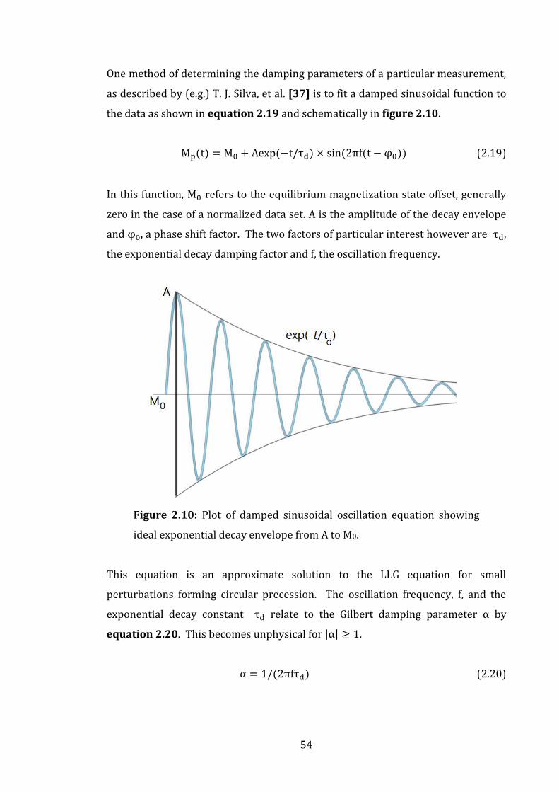
54
One method of determining the damping parameters of a particular measurement,
as described by (e.g.) T. J. Silva, et al. [37] is to fit a damped sinusoidal function to
the data as shown in equation 2.19 and schematically in figure 2.10.
Mp(t) = M0 + Aexp(−t/τd) × sin(2πf(t − φ0)) (2.19)
In this function, M0 refers to the equilibrium magnetization state offset, generally
zero in the case of a normalized data set. A is the amplitude of the decay envelope
and φ0, a phase shift factor. The two factors of particular interest however are τd,
the exponential decay damping factor and f, the oscillation frequency.
Figure 2.10: Plot of damped sinusoidal oscillation equation showing
ideal exponential decay envelope from A to M0.
This equation is an approximate solution to the LLG equation for small
perturbations forming circular precession. The oscillation frequency, f, and the
exponential decay constant τd relate to the Gilbert damping parameter α by
equation 2.20. This becomes unphysical for |α| ≥ 1.
α = 1/(2πfτd) (2.20)
55
The precessional frequency can also be determined from a fast Fourier transform
(FFT) calculation [38]. This provided an independent verification method and was
capable of identifying multiple resonant frequencies which may exist within the
data, as well as the strength of a given frequency, represented by the amplitude of
the frequency spectrum peak [39]. These FFTs were calculated using Origin Lab’s
signal processing functions, with a Hamming filter and fixed sampling intervals.
Amplitude, frequency and full-width half-maximum data was produced from this
and used in conjunction with the damped sinusoidal fit.
2.5 References
[1] Alex Hubert and Rudolf Schäfer, Magnetic Domains: The Analysis of Magnetic
Microstructures (Springer Verlag, Berlin, 1998)
[2] Petros N. Argyres, Phys. Rev. 92, 334 (1955)
[3] Oliver S. Heavens and Robert W. Ditchburn, Insight into Optics (Wiley,
Chichester, 1991)
[4] Fabio Pulizzi, Spintronics, Nature Materials Insight 11, 367 (2012)
[5] Andrei Kirilyuk, Alexey V. Kinel, and Theo Rasing, Rev. Mod. Phys. 82, 2731
(2010)
[6] M. Djordjevic, et al., Phys. Stat. Sol. 3, 1347 (2006)
[7] John Kerr, Phil. Mag., 3, 321 (1877)
[8] P. Weinberger, Phil. Mag. Lett., 88, 897 (2008)
[9] John Kerr, Phil. Mag., 5, 161 (1878)

56
[10] J. C. Maxwell, Phil. Trans R. Soc. Lond., 155, 459 (1865)
[11] M. Mansuripur, The Principles of Magneto-Optical Recording (Cambridge
University Press, Cambridge, 1995)
[12] David J. Griffiths, Introduction to Electrodynamics. 3rd Ed. (Pearson Education,
Inc., 2008)
[13] M. Mansuripur, The Magneto-Optical Kerr Effect, (Optics & Photonics News,
2000)
[14] Joachim Stöhr, Hans C. Siegmann, Magnetism, (Solid-State Sciences Springer
Verlag, Berlin, 2006)
[15] Bert Koopmans, Topics Appl. Phys. 87, 253 (2003)
[16] M. B. Agranat et al., Sov. Phys. JETP 59, 804 (1984)
[17] A. Vaterlaus et al., J. Appl. Phys. 67, 5661 (1990)
[18] A. Vaterlaus et al., Phys. Rev. Lett. 67, 3314 (1991)
[19] A. Vaterlaus et al., Phys Rev. B. 46, 5280 (1992)
[20] E. Beaurepaire, et al., Phys. Rev. Lett. 76, 4250 (1996)
[21] J. Hohlfeld, et al. Phys. Rev. Lett. 78, 4861 (1997)
[22] A. Scholl, et al., Phys. Rev. Lett. 79, 5146 (1997)
[23] B. Koopmans, et al., Phys. Rev. Lett. 85, 844 (2000)

57
[24] M. Aeschlimann, et al., Phys. Rev. Lett. 79, 5158 (1997)
[25] R. Wilks, et al., J. Appl. Phys. 95, 7441 (2004)
[26] P. M. Oppeneer and A. Liebsch, J. Phys.: Condens. Mat. 16, 5519 (2004)
[27] E. Beaurepaire, et al., Phys. Rev. B, 58 12134 (1998)
[28] L. Guidoni, et al., Phys. Rev. Lett., 89, 017401-1 (2002)
[29] J-Y. Bigot, et al., Phys. Rev. Lett. 93, 077401 (2004)
[30] Y. Tserkovnyak, et al., Rev. Mod. Phys. 77, 1375 (2005)
[31] T Gilbert, IEEE Trans. Mag. 40, 3443 (2004)
[32] D.L. Mills and R. Arias, Physica B 384, 147 (2006)
[33] J. Lindner, et al., Phys. Rev. B, 68, 060102(R) (2003)
[34] M. Sparks, R. Loudon and C. Kittel, Phys. Rev. 122, 791 (1961)
[35] C. H. Back, et al., Science 285, 864 (1999)
[36] T. Gerrits, et al., Nature (London) 418, 509 (2002)
[37] T. J. Silva, et al., J. Appl. Phys., 85, 7849 (1999)
[38] A. Mekonnen, et al. Phys. Rev. Lett., 107, 117202 (2011)
[39] E. Brigham, The Fast Fourier Transform and its Applications (Englewood
Cliffs, 1988)

58
Chapter 3
Materials for Spintronic Applications
3.1 Introduction
The core of any spintronic application is the choice of materials. Understanding this
foundation is prerequisite to any meaningful developments in device fabrication
and functionality and the list of useful materials is vast and diverse. This thesis and
this chapter have been focused on two such materials of current interest: the half-
metal, Fe3O4 (magnetite), and the rare-earth transition metal GdFe. This chapter
will detail the physical properties of both of these materials which make them
interesting and useful.
3.2 Half-Metals: Magnetite (Fe3O4)
3.2.1 Structure & Magnetic Properties
Bulk magnetite exists as an inverse spinel cubic structure of lattice constant 0.8397
nm consisting of Fe2+ and Fe3+ ions surrounding an fcc O sublattice [1]. The Fe ions
are arranged in tetrahedral (A) and octahedral (B) sites within the lattice, with 8
Fe3+ ions on A sites and 16 Fe2+/3+ ions occupying B sites to give a resultant charge
here of Fe2.5+. Being a cubic structure, the three most common orientations to find
it are (001), (011) and (111) as displayed in profile in figure 3.1 below. The lattice

59
unit cell consists of 8 planes along the <100> direction, alternately containing A sites
and B sites, with the oxygen sublattice sitting along the planes containing the B site
iron [2]. As can be seen here, the (011) orientation is the only one which fully
resolves the oxygen (red) from the iron atoms (blue).
Figure 3.1: Illustrations of the three most common orientations of the
Fe3O4 cubic inverse spinel crystal unit cell. The structure is comprised of
a fcc O2+ lattice ((O), red atoms), equal numbers of Fe3+ and Fe2+ ions
filling half of the octahedral site ((B), dark blue atoms) and Fe3+ ions
filling ⅛ of the tetrahedral sites ((A), light blue atoms). These
orientations provide different visibility of atomic columns.
Bonding between neighbouring ions in a magnetite crystal lattice is described by the
exchange interaction. This can occur as cation-cation bonding and cation-anion-
cation bonding; corresponding to Fe-Fe and Fe-O-Fe bonding and is described by the
Heisenberg exchange Hamiltonian as follows:
Hex = − ∑ JexSi ∙ Sjij (3.1)
In the above equation Sn represents the spin angular momentum of ion i or j. Jex is
the effective exchange integral, dependent on the angle, distance, spin and electronic
configuration of neighbouring ions i and j. A set of semi-empirical rules were laid
(001) (011) (111)
A O B

60
out in the 1950s by Goodenough and Kanamori [3] [4] determining the properties
of each of these interactions. They take into consideration the electronic symmetry
and occupancy of overlapping atomic orbital wave functions and generally allow a
quick prediction of the net magnetic exchange. However in the case of magnetite
there exists a more complicated system involving competing direct and
superexchange interactions, which define its magnetic character.
Figure 3.2: Cartoons of interatomic interactions which exist in
crystalline magnetite (left) and example positions of superexchange
interactions within the magnetite unit cell (right), displaying (i) ~90
weakly ferromagnetic superexchange interaction on B sites, (ii)
ferromagnetic double exchange interaction on B sites, and (iii) strongly
antiferromagnetic superexchange interaction between octahedral and
tetrahedral iron sites.
These interactions in magnetite occur due to the arrangement of Fe2+ and Fe3+ ions
which have, respectively, 3d6 and 3d5 electronic configurations. The Fe3+ ions have
five unpaired 3d electrons forming a closed subshell and the Fe2+ ions have an extra
electron which results in four 3d electrons unpaired. A local double exchange
61
interaction exists between the B site Fe2+ and Fe3+ ions whereby the direct exchange
of an electron to the empty d level in Fe3+ results in a weak ferromagnetic
contribution. This is mostly masked by much stronger indirect superexchange
interactions, which occur between next nearest neighbour (NNN) Fe ions via a ‘go-
between’ O2-. As there are now three particles involved, the angle between them
becomes an important factor in determining the strength and sign of the interaction.
Super-exchange occurs only between overlapping orbitals with similar symmetry
types and in magnetite there are three 2p orbitals on the O2- ions which can
contribute, consisting of two with π-type and one with σ-type symmetry. On the Fe
ions, there are five 3d orbitals, three with π-type and two with σ-type symmetry, so
when these respectively overlap with the corresponding orbitals of the O2- ions, the
interaction takes place. The σ-type symmetry is generally larger and more dominant
[5]. The two main superexchange interactions in bulk magnetite which must be
considered are: ~120 ̊ FeB-O-FeA (strongly antiferromagnetic) and ~90 ̊ FeB-O-FeB
(weakly ferromagnetic) as shown in figure 3.2.
There are 3 classes of spin-polarisation and magnetite belongs to the second [6],
type IIB, due to it exhibiting hopping within the minority spin band. The conduction
occurs across the B site Fe ions, between the Fe2+ and Fe3+ charges. As discussed
previously, the 5 d-orbital electrons form a closed subshell, leaving the single 6th
electron from the Fe2+ with an opposite spin and in a higher energy level. This single
electron state forms the conduction band at the Fermi level and as such the
conduction is theoretically 100% spin-polarised for a perfect inverse spinel
structure. Literature suggests that magnetite behaves under the itinerant electron
model more so than the localised electron model [7]. A complete understanding of
the complex band structure of magnetite is still unknown, consisting of hybridised
bands of overlapping wave functions. As a material is grown as a nanoscale film, the
properties of the substrate become important and surface effects begin to dominate
the overall characteristics of the material. Surface properties can be significantly
different from those of the bulk, perhaps exhibiting persisting order beyond the
Curie temperature [8]. Theoretical calculations of thin-film systems are possible,
but can be notoriously difficult. Any mismatch in the lattice parameter between film

62
and substrate becomes critical as this can cause defects within the film which also
alter the bulk properties.
3.2.3 Single Crystal Growth Considerations
Iron oxide is stable across a significant range of stoichiometry [9]. A solid solution
group exists with Fe3O4 at one end and γ-Fe2O3 (maghemite) at the other via FeO
(wüstite) and α-Fe2O3 (hematite), following the formula Fe3-δO4 (δ = 0 ↔ 1/3).
wüstite exists in the form Fe1-xO, in a halite (rock-salt) crystal structure whose lattice
parameter is 0.433 nm. It is insulating and antiferromagnetic, with a Néel
temperature (TN) of only 198 K. Hematite exists in an insulating Rhombohedral
lattice structure like Corundum which exhibits antiferromagnetic behaviour
(TN~955 K) and has a band gap of ~2 eV.
Critically maghemite and magnetite share a very similar spinel structure, difficult to
distinguish in structural investigation. Maghemite is a ferrimagnetic insulator with
a band gap of ~2.5 eV and a moment of ~1.2μB. By contrast, magnetite has a very
small band gap of ~0.1 eV [10] and about 20% larger magnetic moment of ~1.4μB.
As a consequence of the shared structure between magnetite and maghemite,
altering oxidization conditions can change the occupation on the octahedral sites of
the spinel lattice from Fe2+ ions to Fe3+ ions and vacancies. This range of conditions
will have a significant effect on the performance of the material as both its
ferrimagnetism and spin polarization rely on the existence of the Fe2+ ions on the
octahedral sites.
For epitaxial single crystal growth, the lattice match between the magnetite unit cell
and that of the chosen substrate must have a very low mismatch. This investigation
will focus on the insulating rock salt, magnesium oxide, MgO (001), which boasts a,
close to, ideal mismatch to Fe3O4 of 0.3%. The lattice constant of MgO is 0.4212 nm,
[11] compared to Fe3O4 of 0.8397 nm, which results in four MgO unit cells matching
to each Fe3O4 unit cell face and continuing the oxygen sublattice. These unit cells
are shown to scale below in figure 3.3.

63
Figure 3.3: Cartoon of (a) Fe3O4 (001) unit cell, containing octahedral
(dark blue) and tetrahedral (light blue) iron ions, showing
superexchange bonds via oxygen (red) sublattice. By comparison, to
scale (b) MgO (001) unit cell, containing magnesium (yellow) sublattice
bonded to oxygen (red) sublattice.
During epitaxial growth, the film is deposited on the substrate piecemeal, at a rate
determined by the sublimation of a growth source. As clusters of Fe3O4 form, they
lower the local surface potential, resulting in island growth with multiple unrelated
nucleation sites. This naturally results in regions of the film where the Fe3O4 unit
cell cannot be tessellated perfectly. The boundaries where these islands meet
cannot always match and defects are formed. These defects are referred to as anti-
phase domain boundaries (APBs) which introduce a greater antiferromagnetic
coupling component [12]. They exist in Fe3O4/MgO (001) for two reasons: the half-
sized unit cell of MgO means that islands can form half a unit cell mismatched, and
the lower order of rotational symmetry of Fe3O4 allows islands to meet 90° rotated
with respect to each other. A crystallographic study of this is reported by S.Celotto,
W. Eerenstein and T. Hibma [13], which discusses the type of defects which are
allowed to occur and their electron microscopy visibility criteria, as calculated by

64
the Howie-Whelan visibility criteria (equation 3.2) and shown in figure 3.4. These
criteria are discussed in more detail in chapter 4.
2πg. R = (2N + 1)π (3.2)
Figure 3.4: Schematic illustration of APB types with shift vectors (left)
showing translational and rotational shifts used to calculate TEM
visibility conditions and 220 type TEM dark field images of APBs in
Fe3O4/MgO (001) films of (a) 6nm, (b) 12nm, (c) 25nm and (d) 50nm
thickness (right).
3.3 Rare Earth-Transition Metal Alloys: GdFe
3.3.1 Structure & Magnetic Properties
Rare earth-transition metal (RE-TM) alloys have enjoyed dedicated study within the
magnetic storage industry for over 40 years, following the ground-breaking paper
of P. Chaudhari, et al. in 1972 [14]. This industrial development brought RE-TM
alloys to market in the first commercial magneto-optic storage devices as the now
superseded ‘bubble memory’. This non-volatile storage technology was considered
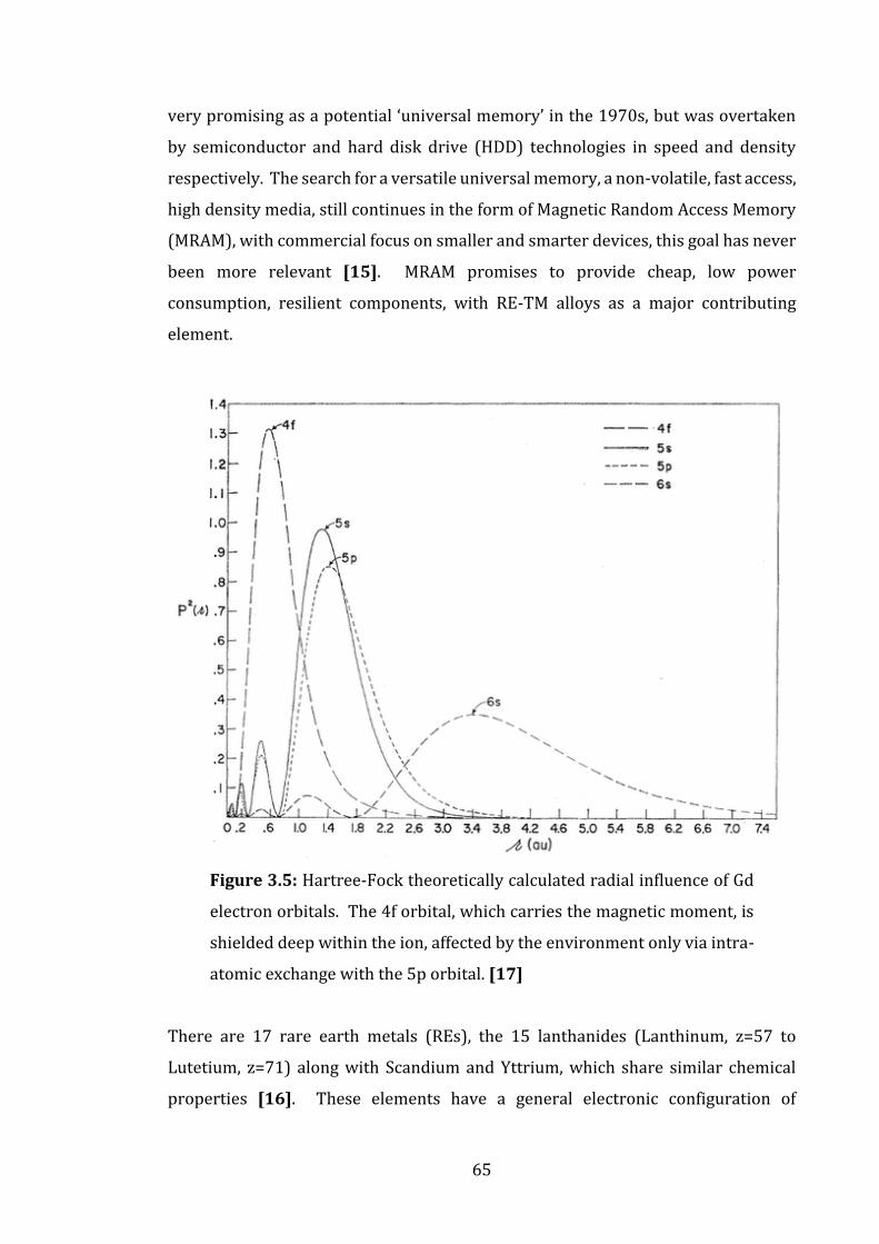
65
very promising as a potential ‘universal memory’ in the 1970s, but was overtaken
by semiconductor and hard disk drive (HDD) technologies in speed and density
respectively. The search for a versatile universal memory, a non-volatile, fast access,
high density media, still continues in the form of Magnetic Random Access Memory
(MRAM), with commercial focus on smaller and smarter devices, this goal has never
been more relevant [15]. MRAM promises to provide cheap, low power
consumption, resilient components, with RE-TM alloys as a major contributing
element.
Figure 3.5: Hartree-Fock theoretically calculated radial influence of Gd
electron orbitals. The 4f orbital, which carries the magnetic moment, is
shielded deep within the ion, affected by the environment only via intra-
atomic exchange with the 5p orbital. [17]
There are 17 rare earth metals (REs), the 15 lanthanides (Lanthinum, z=57 to
Lutetium, z=71) along with Scandium and Yttrium, which share similar chemical
properties [16]. These elements have a general electronic configuration of
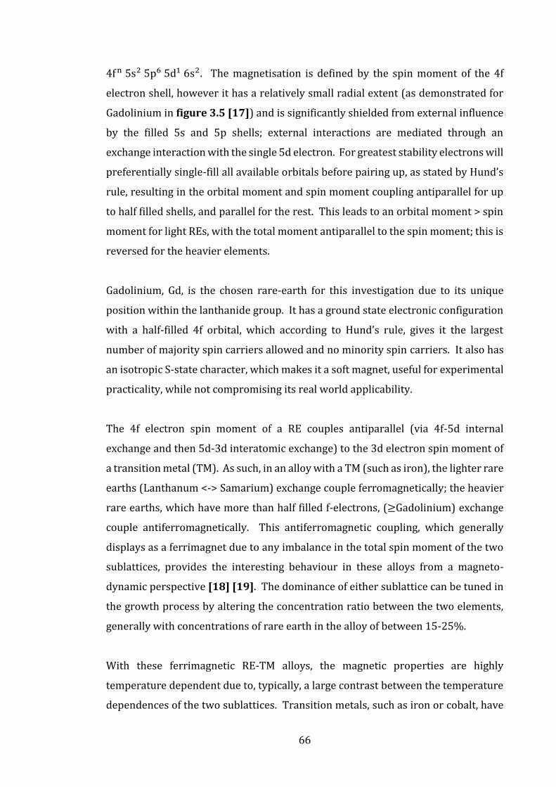
66
4f n 5s2 5p6 5d1 6s2. The magnetisation is defined by the spin moment of the 4f
electron shell, however it has a relatively small radial extent (as demonstrated for
Gadolinium in figure 3.5 [17]) and is significantly shielded from external influence
by the filled 5s and 5p shells; external interactions are mediated through an
exchange interaction with the single 5d electron. For greatest stability electrons will
preferentially single-fill all available orbitals before pairing up, as stated by Hund’s
rule, resulting in the orbital moment and spin moment coupling antiparallel for up
to half filled shells, and parallel for the rest. This leads to an orbital moment > spin
moment for light REs, with the total moment antiparallel to the spin moment; this is
reversed for the heavier elements.
Gadolinium, Gd, is the chosen rare-earth for this investigation due to its unique
position within the lanthanide group. It has a ground state electronic configuration
with a half-filled 4f orbital, which according to Hund’s rule, gives it the largest
number of majority spin carriers allowed and no minority spin carriers. It also has
an isotropic S-state character, which makes it a soft magnet, useful for experimental
practicality, while not compromising its real world applicability.
The 4f electron spin moment of a RE couples antiparallel (via 4f-5d internal
exchange and then 5d-3d interatomic exchange) to the 3d electron spin moment of
a transition metal (TM). As such, in an alloy with a TM (such as iron), the lighter rare
earths (Lanthanum <-> Samarium) exchange couple ferromagnetically; the heavier
rare earths, which have more than half filled f-electrons, (≥Gadolinium) exchange
couple antiferromagnetically. This antiferromagnetic coupling, which generally
displays as a ferrimagnet due to any imbalance in the total spin moment of the two
sublattices, provides the interesting behaviour in these alloys from a magneto-
dynamic perspective [18] [19]. The dominance of either sublattice can be tuned in
the growth process by altering the concentration ratio between the two elements,
generally with concentrations of rare earth in the alloy of between 15-25%.
With these ferrimagnetic RE-TM alloys, the magnetic properties are highly
temperature dependent due to, typically, a large contrast between the temperature
dependences of the two sublattices. Transition metals, such as iron or cobalt, have
67
a high Curie temperature (1043 K, 1400 K respectively) compared to that of the rare
earths. Due to the separate origins of the magnetization in RE and TM (4f shell and
3d shell respectively), the magnetic moments of each sublattice retain separate
temperature dependencies. The localized 4f shell moment produces a larger
temperature dependence than that of the itinerant 3d shell; as a result, at low
temperatures, typically, the magnetic moment of the RE will dominate that of the
TM, and vice versa for high temperatures.
Figure 3.6: Schematic guide to the temperature dependence of both
individual sublattices along with their combined effect on the net
magnetic characteristics of the material. Shows the two compensation
temperatures, magnetic (TM) and angular momentum (TA) along with the
Curie temperature (TC) these broadly describe the temperature
dependent characteristics of a RE-TM material. [20]

68
The temperature at which the RE and TM spin moments are balanced is referred to
as the magnetization compensation temperature, TMcomp and will generally be
reduced with increased RE concentration in the alloy. At this point (as shown in
figure 3.6) there is a divergence in the coercive field, Hc, required to switch the
magnetization, which is due to the relationship Hc = 2K/MS [21] and the observation
that at this point there is a drastic reduction in net magnetic moment, M, without
loss of intrinsic magnetic anisotropy, K. This means that around this temperature,
it becomes extremely energetically expensive to manipulate the magnetic ordering
of the alloy. For spintronic applications, alloys with TMcomp around or just above
room temperature are ideal as at this point, the magnetic state, and thus the stored
information, is greatly resistant to unwanted stray fields.
Analogously to TMcomp an angular momentum compensation temperature TAcomp can
be defined where the contributions of the two sublattices are equal and opposite,
cancelling each other. This compensation is due to the composition dependence of
each sublattice’s gyromagnetic ratios (which relate the magnetic moment to angular
momentum) and will vary relative to TMcomp for different elements and composition
ratios. As discussed in chapter 2 it is the angular momentum contribution which
significantly impacts on magneto-dynamic rates and is thus a critical parameter for
any applied technology.
3.3.2 Magneto-dynamic Properties
A general theory of laser-induced ultrafast demagnetisation considers a unified
material with a single temperature dependence (see chapter 2). Experimental
evidence [22] however suggests that in the special case of a ferrimagnetic multi-
sublattice material, such as GdFe, the two sublattices undergo distinct ultrafast
dynamic behaviour. Experimental and theoretical evidence has been reported [23]
[24] in which magnetic switching is achieved using linearly polarized light, caused
by a transient “ferromagnetic-like state” in which the RE and TM sublattices align
parallel on a picosecond timescale. Recent work by Mentink et al. [25] attributed
this to an additional angular momentum exchange between the sublattices, not
possible in a single sublattice material. In this treatment, the two-temperature
69
model of electron and lattice thermal reservoirs is accepted and defines three
regimes of dynamics relative to the electron temperature: Te >>Tc, Te~Tc and Te<Tc.
Above the Curie temperature, the system is paramagnetic; the interaction between
sublattices can be considered negligible and their dynamics independent. Crucially,
this initial relaxation rate is calculated to be dependent on the atomic magnetic
moment. Once the temperature drops to the vicinity of Tc, angular momentum
exchange between the sublattices begins to occur alongside intra-sublattice
relaxation, and gradually comes to dominate the dynamics. This leads to the
conclusion that the interplay between two antiferromagnetically bound sublattices
causes a mutual acceleration of the demagnetization process.
Further treatment of RE-TM dynamics came from Wienholdt et al. (2013) figure 3.7
[26] who proposed an “orbital-resolved spin model” separating the dynamics of the
4f and 5d electrons within the RE sublattice. As discussed previously, it is the 4f
electrons that carry the most (92%) magnetic moment in a RE, but are buried deep
beneath the Fermi energy accessible only through exchange with the 5d electron
shell. This 5d shell can be thermally excited by laser heating, but the 4f cannot.
After laser heating and electron thermalization, strong spin non-equilibrium will
exist between the directly accessible transition metal 3d spins and the shielded rare
earth 4f spins. In order to maximize entropy, as the exchange interaction begins to
compete, angular momentum transfer will occur not only between the two
sublattices but also within the RE sublattice. The TM sublattice will reach its (laser
fluence dependent) maximum demagnetization state after ~1 ps while the RE
sublattice is still demagnetizing, leading to a transient state in which both spin
systems are aligned. This leads to a faster demagnetization process than single
sublattice relaxation.

70
Figure 3.7: Schematic demonstration of the energy transfer channels
which exist within a RE-TM alloy under laser photon stimulation and
theoretical calculated response rates for Gd5d, Fe3d and Gd4f electron
orbitals. [26]
Recent work by Stanciu et al. (2006) figure 3.8(c) [27] and Mekonnen et al. (2011)
figure 3.8 (b) [28] has reported fluence dependent investigations on RE-TM alloys,
providing experimental evidence of the inter-sublattice exchange occurring. These
papers show that the frequency of precessional spin motion is related to the
strength of the coupling between the sublattices and their ability to transfer energy
and angular momentum. In this work, the coherent macrospin precession (referred
to as the ferromagnetic resonance FMR mode) is shown to clearly respond to the
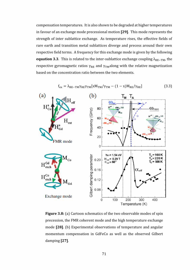
71
compensation temperatures. It is also shown to be degraded at higher temperatures
in favour of an exchange mode precessional motion [29]. This mode represents the
strength of inter sublattice exchange. As temperature rises, the effective fields of
rare earth and transition metal sublattices diverge and precess around their own
respective field terms. A frequency for this exchange mode is given by the following
equation 3.3. This is related to the inter-sublattice exchange coupling λRE−TM, the
respective gyromagnetic ratios γRE and γTMalong with the relative magnetization
based on the concentration ratio between the two elements.
fex = λRE−TMγREγTM[xMTM/γTM − (1 − x)MRE/γRE] (3.3)
Figure 3.8: (a) Cartoon schematics of the two observable modes of spin
precession, the FMR coherent mode and the high temperature exchange
mode [28]. (b) Experimental observations of temperature and angular
momentum compensation in GdFeCo as well as the observed Gilbert
damping [27].

72
3.4 Summary
In summary, the magnetic properties of Fe3O4 are highly dependent upon its
crystallographic ‘purity’ making the growth process a very key aspect of any quality
refinement. The crystal benefits from a high spin-polarizability and high Curie
temperature, while requiring only cheap and abundant elements. These make this
a worthwhile cause. The quality of the material can be analysed in detail by electron
microscopy and provide feedback to the growth process.
The RE-TM alloy, by contrast, has no restriction on crystal geometry and as such is
easier to produce and alter the composition ratio for material performance
optimization. Their angular momentum and magnetization compensation points
make them ideal for long term stable storage of magnetic information and make
temperature dependent studies an informative method of characterization.
3.5 References
[1] A. Koblischka-Veneva, et al., J. Appl. Phys. 103, 07E505 (2008)
[2] V. K. Lazarov, et al., Phys. Rev. B, 72, 195401 (2005)
[3] J. B. Goodenough, Phys. Rev., 100, 564 (1955)
[4] J. Kanamori, J. Phys. Chem. Solids 10, 87 (1959)
[5] K. Yosida, Theory of Magnetism (Springer-Verlag, Berlin, 1996)
[6] G. M. Müller, Nature Mat., 8, 56 (2009)

73
[7] M. Kallmeyer, et al. J. Appl. Phys., 103, 07D715 (2008)
[8] L. M. Falicov, Thin Solid Films, 216, 169 (1992)
[9] M. Paul et al. J. Appl. Phys., 110, 073519 (2011)
[10] R. M. Cornell and U. Schwertmann, The Iron Oxides: Structure Properties,
Reactions, Occurrences and Uses, (Wiley-VCH 2003)
[11] R. J. Beals, et al., J. Am. Ceram. Soc., 40, 279 (1957)
[12] D.T. Margulies, et al., Phys. Rev. Lett., 79, 5162 (1997)
[13] S. Celotto, W. Eerenstein, and T. Hibma, Eur. Phys. J. B, 36, 271 (2003)
[14] P. Chaudhari, et al., Appl. Phys. Lett., 22, 337 (1973)
[15] US patent US 7531830 B2 “Spin-polarization devices using rare earth-
transition metal alloys” (2007)
[16] G. R. Giesbrecht and J. C. Gordon, Dalton Trans. 2387 (2004)
[17] A. J. Freeman and R. E. Watson., Phys. Rev., 127, 2058 (1962)
[18] M. Mansuripur, The Physical Principles of Magneto-Optical Recording
(Cambridge University Press, Cambridge, 1995)
[19] X. Jiang, et al., Phys. Rev. Lett., 97, 21702 (2006)
[20] C. D. Stanciu, Laser-Induced Femtosecond Magnetic Recording (PhD Thesis,
Radboud University, Nijmegen, The Netherlands, 2008)

74
[21] J. D. Livingston, J. Appl. Phys. 52, 2544 (1981)
[22] C. Stamm et al., Nature Mater. 6, 740 (2007)
[23] I. Radu, et al. Nature (London) 472, 205 (2011)
[24] T. A. Ostler, et al. Nat. Commun. 3, 666 (2012)
[25] J. H. Mentink, et al., Phys. Rev. Lett., 108, 057202 (2012)
[26] S. Weinholdt, et al., Phys. Rev. B, 88, 020406(R) (2013)
[27] C. D. Stanciu, et al., Phys. Rev. B, 73, 220402(R) (2006)
[28] A. Mekonnen, et al., Phys. Rev. Lett., 107, 117202 (2011)
[29] J. Kaplan and C. Kittel, J. Chem. Phys., 21, 760 (1953)

75
Chapter 4
Quality Control of Materials
4.1 Introduction
This chapter discusses the techniques and principles necessary to produce and
characterize the material quality of a test sample and has been subdivided by
discipline. Molecular beam epitaxy growth method and technique used to produce
thin-film Fe3O4 samples for this project in the Department of Physics at York are
discussed, along with a brief comparison to sputter deposition used undertaken by
collaborators for GdFe alloy thin-films also investigated. Facilities available at the
York-Jeol Nanocentre for electron microscopy imaging of thin-films, as well as the
techniques used and developed over the course of this project are then detailed.
4.2 Growth Techniques
4.2.1 Molecular Beam Epitaxy (MBE)
As implied by the name, MBE employs concentrated beams of molecules or atoms,
which are liberated from a source by sublimation heating and directed through an
ultra-high vacuum (UHV) (<10-9 mbar) to an atomically flat crystalline substrate.

76
This beam, with a low flux, creates a uniform film one layer at a time. Originally
applied to compound semiconductor growth, today it is used to produce thin-films
of a large number of material types. The UHV environment maintains the purity of
the substrate surface and because the mean free path of the beam is much greater
than the distance between source and substrate, it will be extremely uniform in
energy and incidence angle. Furthermore, any scattered molecules will be captured
by the walls of the chamber and removed from the growth. A raised temperature of
the substrate allows arriving molecules the thermal energy required to shift across
its surface onto lattice sites, facilitating the underlying crystal structure to translate
to the grown film. If the crystalline structure of the substrate translates to that of
the film, it is considered to be epitaxial. A mechanical shutter is used to produce
sharp start and end times to film deposition, in this manner numerous film layers of
differing constitution can be grown on top of one another and each time the
molecular beam flux can be tuned to a desired deposition rate before the substrate
is exposed. Figure 4.1 shows a schematic of the growth chamber.
Samples are loaded into the chamber via a fast entry load lock and manoeuvred into
position above the sublimation sources. The base pressure in the growth chamber
is kept below 10-10 mbar, which can rise as high as 10-5 mbar during growth.
Deposition can be controlled to an accuracy of 0.05 nm/min and the substrate can
be heated to above 1000 ̊C via a tungsten filament and electron beam heating. All
substrates were thoroughly cleaned, prior to insertion into the growth chamber,
using acetone, then ethanol.
The important differentiating factor between this method and other growth systems
is the rate of deposition; which is much lower here than in, for example, plasma
sputtering systems. This slower rate, in theory, allows more precise control over
the thickness of the film over a range from 1-100 nm and, more importantly,
epitaxial single-crystal growth. In order to accommodate this slower growth rate
which would allow more impurity collisions, the apparatus must be contained
within a proportionally higher vacuum system.

77
Figure 4.1: Schematic of MBE system. The sample is positioned at the
top of the chamber behind a mechanical shutter. An electron source gun
is guided onto a sublimation source in a Hearth, which ejects a molecular
beam towards the sample. Various pumps and heat sinks are used to
maintain the low pressure environment. A plasma oxygen source is
fitted here to introduce molecular oxygen into the chamber for post-
oxidation experiments.
A piezoelectric quartz crystal rate monitor is used to measure the rate of deposition
during a growth procedure. As the vibrational frequency of the crystal is
proportional to its mass, it is placed in position to receive an equivalent amount of
deposited material as the substrate. By referring to the molecular mass of the
sublimation source, it is possible to track the thickness of a grown film quite
accurately, to within one or two monolayers.
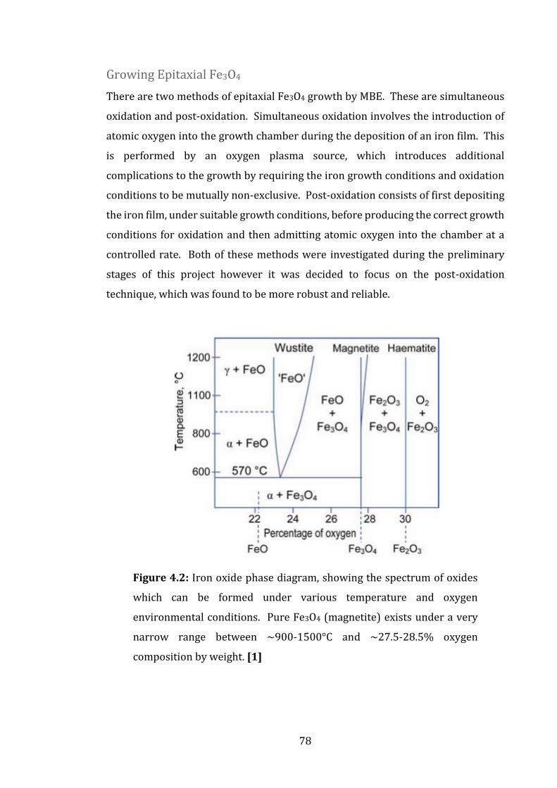
78
Growing Epitaxial Fe3O4
There are two methods of epitaxial Fe3O4 growth by MBE. These are simultaneous
oxidation and post-oxidation. Simultaneous oxidation involves the introduction of
atomic oxygen into the growth chamber during the deposition of an iron film. This
is performed by an oxygen plasma source, which introduces additional
complications to the growth by requiring the iron growth conditions and oxidation
conditions to be mutually non-exclusive. Post-oxidation consists of first depositing
the iron film, under suitable growth conditions, before producing the correct growth
conditions for oxidation and then admitting atomic oxygen into the chamber at a
controlled rate. Both of these methods were investigated during the preliminary
stages of this project however it was decided to focus on the post-oxidation
technique, which was found to be more robust and reliable.
Figure 4.2: Iron oxide phase diagram, showing the spectrum of oxides
which can be formed under various temperature and oxygen
environmental conditions. Pure Fe3O4 (magnetite) exists under a very
narrow range between ~900-1500°C and ~27.5-28.5% oxygen
composition by weight. [1]

79
The factors which contribute to the oxide formation are iron deposition rate, growth
temperature, oxygen partial pressure, oxidation temperature and time [1]. As
discussed in more detail in chapter 3, there is a spectrum of iron oxides which can
be formed during this growth process. Figure 4.2 shows the temperature vs oxygen
percentage chart, which gives an idea of the challenge associated with growing pure
single phase Fe3O4, under a very narrow combination of temperature and pressure
conditions.
4.2.2 Sputter Deposition
A number of sputtering techniques exist, but what they all have in common is a
relatively high growth rate, producing polycrystalline thin-films rather than single
crystals. This method particularly excels over MBE growth in its ability to deposit
materials with high melting points, which would otherwise be difficult to evaporate.
It is a desirable technique for rare earth-transition metal alloy deposition because
of its ability to produce denser films [2]. Factors which affect the growth are the
choice of sputtering gas and gas pressure, as well as deposition rate and
temperature.
Rare earth-transition metal samples created during this investigation were grown
to 20 nm thickness on cleaved 5x10 mm Si substrates at room temperature and
1x10⁻⁷ mbar base pressure. This growth was by direct current magnetron co-
sputtering from elemental targets, using Ar gas at a pressure of ~0.005 mbar, at
Nanjing University, China. The samples were finished with a 5 nm Au cap for
oxidation protection. Composition ratios of Gd:Fe were then controlled by tuning
the relative deposition rates, monitored by quartz crystal rate monitoring.
4.3 Imaging Techniques
With a sample offcut, or once non-invasive characterizations have been undertaken,
investigation of the atomic structure of a sample can give an essential insight into
the physical properties of a thin-film system. As Fe3O4, like many other materials, is
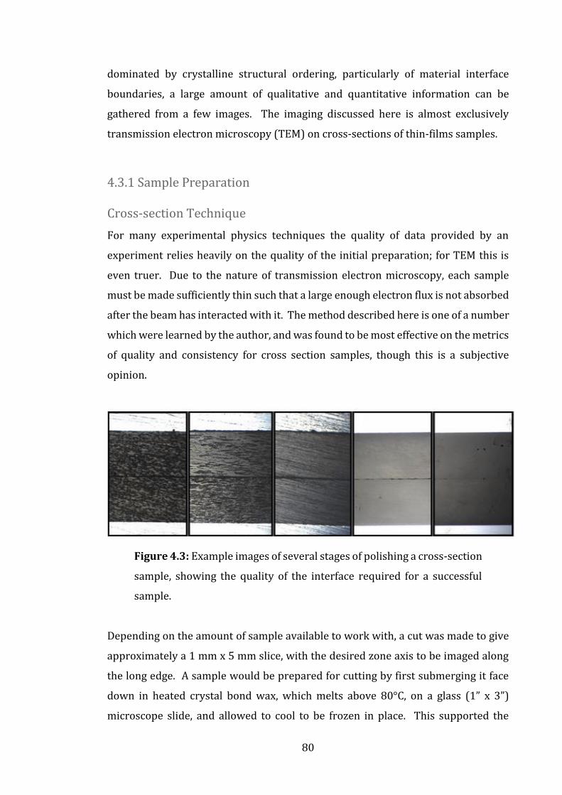
80
dominated by crystalline structural ordering, particularly of material interface
boundaries, a large amount of qualitative and quantitative information can be
gathered from a few images. The imaging discussed here is almost exclusively
transmission electron microscopy (TEM) on cross-sections of thin-films samples.
4.3.1 Sample Preparation
Cross-section Technique
For many experimental physics techniques the quality of data provided by an
experiment relies heavily on the quality of the initial preparation; for TEM this is
even truer. Due to the nature of transmission electron microscopy, each sample
must be made sufficiently thin such that a large enough electron flux is not absorbed
after the beam has interacted with it. The method described here is one of a number
which were learned by the author, and was found to be most effective on the metrics
of quality and consistency for cross section samples, though this is a subjective
opinion.
Figure 4.3: Example images of several stages of polishing a cross-section
sample, showing the quality of the interface required for a successful
sample.
Depending on the amount of sample available to work with, a cut was made to give
approximately a 1 mm x 5 mm slice, with the desired zone axis to be imaged along
the long edge. A sample would be prepared for cutting by first submerging it face
down in heated crystal bond wax, which melts above 80°C, on a glass (1” x 3”)
microscope slide, and allowed to cool to be frozen in place. This supported the
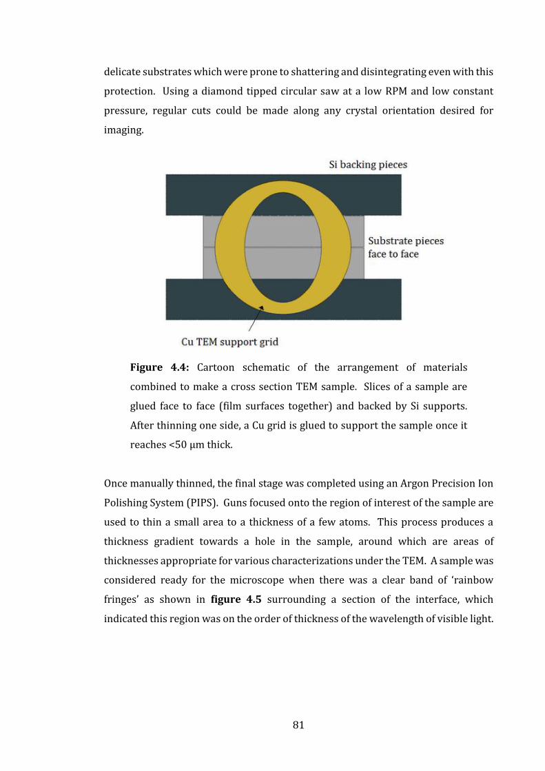
81
delicate substrates which were prone to shattering and disintegrating even with this
protection. Using a diamond tipped circular saw at a low RPM and low constant
pressure, regular cuts could be made along any crystal orientation desired for
imaging.
Figure 4.4: Cartoon schematic of the arrangement of materials
combined to make a cross section TEM sample. Slices of a sample are
glued face to face (film surfaces together) and backed by Si supports.
After thinning one side, a Cu grid is glued to support the sample once it
reaches <50 µm thick.
Once manually thinned, the final stage was completed using an Argon Precision Ion
Polishing System (PIPS). Guns focused onto the region of interest of the sample are
used to thin a small area to a thickness of a few atoms. This process produces a
thickness gradient towards a hole in the sample, around which are areas of
thicknesses appropriate for various characterizations under the TEM. A sample was
considered ready for the microscope when there was a clear band of ‘rainbow
fringes’ as shown in figure 4.5 surrounding a section of the interface, which
indicated this region was on the order of thickness of the wavelength of visible light.

82
Figure 4.5: After PIPS milling, the sample is considered ready when a
clear band of rainbow fringes are observable at the interface. This is due
to the thickness of that region being of the scale order of the wavelength
of visible light.
Plan-View Lift-Off Technique
Information from a sample surface can be useful alongside the cross-section. This
view, especially, gives an advantageous position from which to view the effects of
the island growth and the density of APBs throughout the film. This technique was
developed during the PhD of Dr. Wilma Erenstein [3] as an alternative to a more
traditional plan-view preparation technique detailed above for cross-section. The
method involves the chemical removal of the film from the MgO substrate using
ammonium sulphate ((NH4)2SO4) solution. This allows the film to be retrieved on a
Cu fine mesh grid and placed directly into the microscope. For this process a 10%
solution was made and then used to fill petri dishes suspended in a heat bath. 1x1
mm pieces of a specimen were placed floating on the solution film-side up and the
process was left to run for 24 hours at 70 ̊C. The grid was prepared by soaking in
ethanol and drawing out impurities onto filter paper. After this time, the substrate
had slightly dissolved and detached itself from the film, which was left floating on
the surface of the solution. This process did not yield 100% success, but the quality
of successful samples was very good. Generally the film fragmented and small
samples of this were collected. It was important at this point to carefully wash the
sample in ethanol from a pipette, to reduce the contaminants which otherwise
degraded the quality of TEM images obtainable.

83
4.3.2 Transmission Electron Microscopy (TEM)
Transmission electron microscopy is a technique which allows the detailed probing
of structures down to the atomic scale. The concept was formulated in the early
20th century and the principles of the pioneering apparatus are very similar to the
microscopes used today. The technique shares many similarities with visible light
optics; with the photon source replaced by an electron source, and the physical
lenses replaced with electromagnetic coils. Electron optics allows the probing of
much smaller structures, due to a much smaller de Broglie wavelength. They are
also more strongly interacting with matter due to Coulombic interaction and are
easily channelled because of their charged nature. The main conceptual difference
between electron and light optics comes in the way the resulting images are
produced, relying on diffracted and reflected flux respectively. This requirement
makes sample preparation very important, as the sample must be made thinner than
the penetration depth of the electron beam for any information to be obtained at all.
This depth is dependent on the energy of the beam and the density of the target
sample but is generally on the order of a few nanometres.
A schematic of the electron optics is shown in figure 4.6 above. The electron source
at the top of the column is a tungsten filament, which is shielded on all sides except
for an opening which directs a diffuse beam down through the instrument. Each
lens is an electromagnetic coil encircling the beam line and the condenser lenses
begin by collecting and focusing the beam down onto the sample. At this stage the
intensity and diffuseness of the beam can be controlled by adjusting the
microscope’s focal plane. From this point the beam, carrying the information from
the specimen, passes through the objective lens where it is collected and focused
into a coherent image. Lastly, intermediate and projector lenses refine and direct
the beam onto a phosphor viewing screen or CCD camera system for observation
and recording.
All of the lenses are subject to aberrations due to the engineering challenge of
constructing perfect cylinders to the length scale required, as tiny defects in the
system can have a large impact on the image fidelity. This is rectified by
manipulating the magnetic fields of each coil to correct for any astigmation. In order
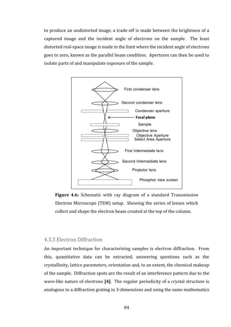
84
to produce an undistorted image, a trade-off is made between the brightness of a
captured image and the incident angle of electrons on the sample. The least
distorted real-space image is made in the limit where the incident angle of electrons
goes to zero, known as the parallel beam condition. Apertures can then be used to
isolate parts of and manipulate exposure of the sample.
Figure 4.6: Schematic with ray diagram of a standard Transmission
Electron Microscope (TEM) setup. Showing the series of lenses which
collect and shape the electron beam created at the top of the column.
4.3.3 Electron Diffraction
An important technique for characterising samples is electron diffraction. From
this, quantitative data can be extracted, answering questions such as the
crystallinity, lattice parameters, orientation and, to an extent, the chemical makeup
of the sample. Diffraction spots are the result of an interference pattern due to the
wave-like nature of electrons [4]. The regular periodicity of a crystal structure is
analogous to a diffraction grating in 3-dimensions and using the same mathematics

85
it becomes possible to make quantified measurements of the dimensions of the
repeating units of that crystal structure. Bragg’s law (equation 4.1) gives a starting
point for understanding this process, for the case where probing electron beams are
parallel and at discrete distances, d, apart. A Bragg peak is produced where
reflections from given crystal planes interact constructively as expressed by the
following equation, in which n is an integer, λ is the wavelength of the incident
electrons and Θ is the angle between incident and scattered rays:
nλ = 2dsinΘ (4.1)
These Bragg peaks are, in practise, the spots seen in a diffraction pattern and the
spacing between these spots correspond directly to reciprocal distances in the
crystal lattice. The theory talks about reflections; however the real life situation in
a TEM is based on diffraction, which provides extra complexity due to multiple
planes being involved, with some existing in the lattice but having ‘forbidden
reflections’. Calculating the real space dimensions of a crystalline structure becomes
straight forward for a known camera length using equation 4.2:
dx = ((nlhklMgO
)/(4lx)). dhkl (4.2)
For example the calibration at 30cm camera length to convert pixels into a real
distance is:
dx= ((18.6961 × 0.2105)/(4 × lx)). dhkl

86
Figure 4.7: Calculated diffraction pattern for Fe3O4 (001) showing the
Miller index for each spot corresponding to a plane in the real-lattice. [5]
The simulated diffraction pattern of Fe3O4 (001) is shown in figure 4.7, produced
by the software package JEMS [5]. This crystallography and electron microscopy
software suite is a database of crystal structures and their associated characteristics.
This was used as a characterisation tool to help with identification of TEM images
and diffraction patterns by facilitating the identification of specific lengths and
angles in crystal structures in different orientations.
Miller indices are given for each spot, indicating the lattice planes they correspond
to (figure 4.8). In a cubic system, these are given an x,y,z vector coordinate (hkl)
and the plane referred to is the one orthogonal to that vector.

87
Figure 4.8: Examples of basic Miller indices for a simple cubic system.
The Digital Micrograph software suite was used to collect and then analyse TEM
images. It provides the means to study scale calibrated images to accurately
measure distances and angles within them. A number of processing tools are
available within the software, for example allowing the user to mask and isolate
sections of an image. It is possible to take a simulated diffraction image from a High-
Resolution TEM (HRTEM) image using a fast Fourier transform (FFT) calculator.
This has benefits and drawbacks based on actual imaging of a diffraction pattern;
the image quality must be high, resolving atomic planes and thickness contrast
artefacts can be unwantedly introduced.
This technique was extremely useful for observing and identifying defects in the
structure of the film, especially around interfaces. Once an HRTEM image was taken,
an FFT was calculated for the entire image. A mask was applied to this, isolating
spots corresponding to the planes under investigation (as a mirrored pair around
the zero-spot). An inverse Fourier Transform (IFFT) was then taken of this,
producing an image which contained only those planes, making defects much easier
to spot.
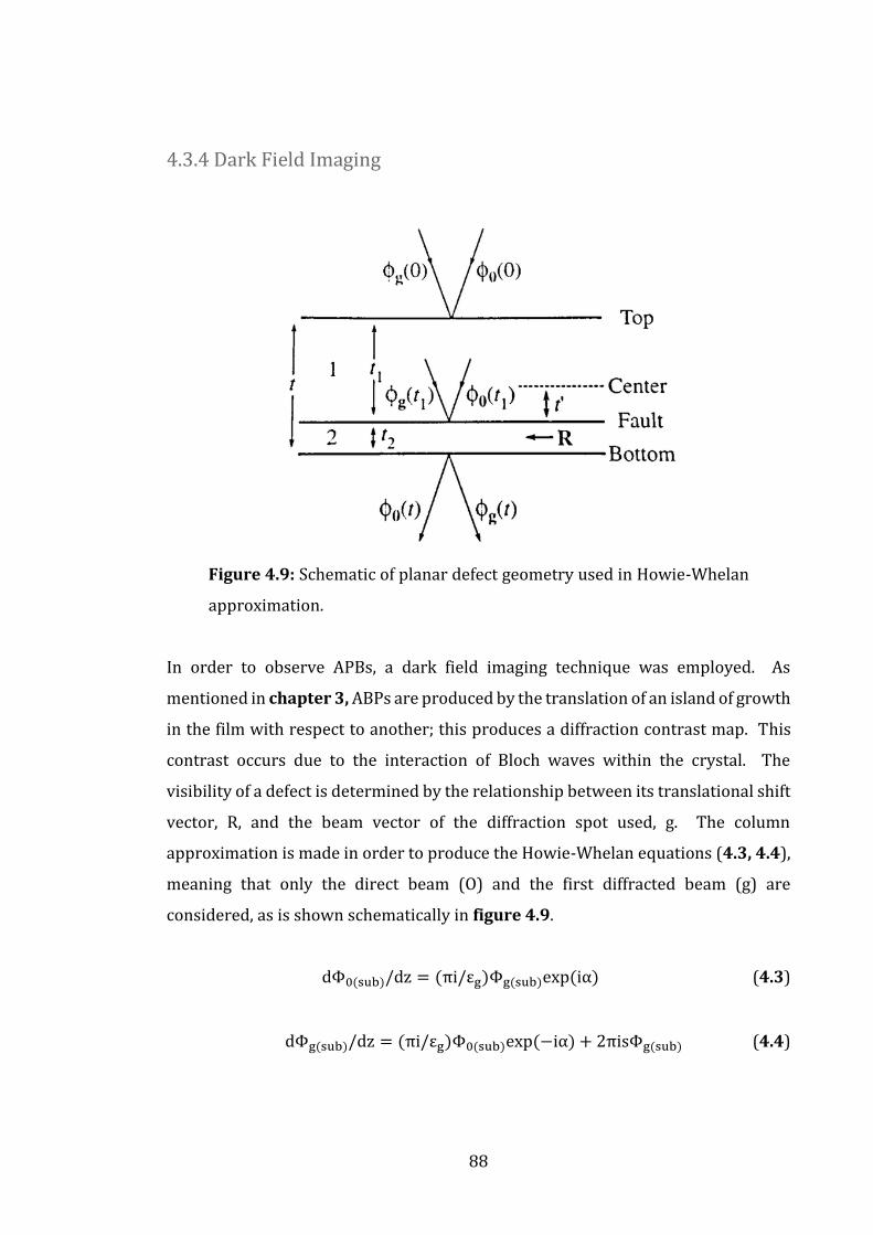
88
4.3.4 Dark Field Imaging
Figure 4.9: Schematic of planar defect geometry used in Howie-Whelan
approximation.
In order to observe APBs, a dark field imaging technique was employed. As
mentioned in chapter 3, ABPs are produced by the translation of an island of growth
in the film with respect to another; this produces a diffraction contrast map. This
contrast occurs due to the interaction of Bloch waves within the crystal. The
visibility of a defect is determined by the relationship between its translational shift
vector, R, and the beam vector of the diffraction spot used, g. The column
approximation is made in order to produce the Howie-Whelan equations (4.3, 4.4),
meaning that only the direct beam (O) and the first diffracted beam (g) are
considered, as is shown schematically in figure 4.9.
dΦ0(sub)/dz = (πi/εg)Φg(sub)exp(iα) (4.3)
dΦg(sub)/dz = (πi/εg)Φ0(sub)exp(−iα) + 2πisΦg(sub) (4.4)

89
In these equations, Φ0 is the amplitude of the direct beam (g=0), Φg is the amplitude
of the diffracted beam for reflection G and εg is the characteristic length for
reflection g, known as the ‘extinction distance’. Planar defects exist when the phase
term, α, is non-zero, which can be rewritten as
α = 2π𝐠. 𝐑 (4.5)
This condition is created experimentally by locating an area of interest on the
sample and then tilting the crystal away from the zone axis so only one strong
diffracted beam remains. This is known as the ’two-beam condition’. At this point
an objective aperture is used to mask all inclusions except those from this diffracted
beam. The defect free areas of the film remain bright and slightly over saturated,
fulfilling the Bragg condition, while locations containing defects bend the beam
away from the beamline and so appear very dark.
The visibility criteria of an APB, as described by W. Eerenstein [3], are as follows:
2πg. R = (2N + 1)π (4.6)
This is approximately the same as for a stacking fault planar defect. In this equation,
g is the diffraction vector of the electron beam, R is the translation vector of the
planar defect as a fraction of the Fe3O4 unit cell. N indicates visibility of an APB for
a chosen diffraction spot if it is an integer and invisibility otherwise.

90
4.4 References
[1] D. R. Lide, Handbook of Chemistry and Physics (88th edition, CRC Press, New
York, USA, 2007)
[2] M. Mansuripur, The Physical Principles of Magneto-Optical Recording
(Cambridge University Press, Cambridge, 1995)
[3] W. Eerenstein, Spin-dependent transport across anti-phase boundaries in
magnetite films (Ph.D Thesis, University of Groningen, 2003)
[4] D. B. Williams and C. B. Carter, Transmission Electron Microscopy: II Diffraction
(Plenum Press, New York, 1996)
[5] JEMS crystallographic analysis software package
http://cimewww.epfl.ch/people/stadelmann/jemsWebSite/jems.html

91
Chapter 5
Building Magnetic Characterization Techniques
5.1 Introduction
During the course of this project, one major set-up was developed; a femtosecond
time-resolved optically-induced pump-probe magneto-optic Kerr effect (MOKE)
apparatus. This work spanned from design of a new lab and commissioning of a
Spectra-Physics femtosecond laser system to a full plan and build of the optics and
construction of detectors and software. Alongside this work, design and
improvement of a number of other instruments, including static high-resolution
MOKE was completed.
5.2 Measuring the Magneto-Optic Kerr Effect (MOKE)
While a number of magneto-optic (MO) effects exist, they are all associated with the
propagation and interaction of an electromagnetic wave with a medium under the
influence of a static or quasi-static magnetic field, producing an observable change
in polarization [1] [2]. Where this wave is able to propagate through the medium,
it is said to have undergone a Faraday Effect rotation, named for its discoverer
Michael Faraday in 1845 who succeeded in providing the first piece of experimental
92
evidence of the relationship between light and magnetism. In the case where the
electromagnetic wave is reflected rather than transmitted through the medium, it is
referred to as the Kerr Effect, named for its discovery by John Kerr in 1877 and
commonly abbreviated to MOKE.
A linearly polarized beam of light, incident on magnetized material experiences an
imbalance in the propagation rate of right and left rotating polarizations, resulting
in a net shift in the polarization angle of the wave. A degree of ellipticity is induced
as the principal axis is rotated relative to the incident beam. The effect is generally
small (~1/1000 rad) so it is critical that the experiment is set up with precision and
stability in mind. It is important to note that the penetration depth of the beam is
on the order of 10 nm - 20 nm and that for films thinner than this, the signal will
decrease proportionally to the thickness.
Within the topic of the Kerr effect, it is necessary to make a further distinction based
on the direction of the magnetization vector, M, of the sample relative to the plane
of incidence. The effect is separated into three: longitudinal, transverse and polar,
representing M in-plane with the plane of incidence and reflection surface;
orthogonal and in-plane; and orthogonal and out-of-plane respectively. Each effect
provides different information about the sample and it is important to be aware
which effects are present in a particular measurement and sample. A more detailed
treatment can be found in chapter 2.
A number of MOKE detection methods exist, based on directing the reflected light
onto a photodiode, which registers a change in intensity as a voltage. The simplest
system relies on a single detector in a configuration known as a cross-analyzer. A
pair of high extinction ratio (>100,000:1) linear polarizers are set at orthogonal
polarizations to each other, one in the incident beam path, and one in the reflected
beam path. These are referred to as polarizer and analyzer, respectively (see figure
5.1). In the case where the magnetization vector of the sample is negligible, the
reflected light is completely extinguished by the analyzer and the detector registers
baseline voltage. From this state, any change in the angle of polarization is detected
as an increase in the intensity of light reaching the detector. This detection is blind
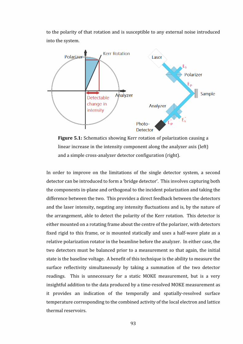
93
to the polarity of that rotation and is susceptible to any external noise introduced
into the system.
Figure 5.1: Schematics showing Kerr rotation of polarization causing a
linear increase in the intensity component along the analyzer axis (left)
and a simple cross-analyzer detector configuration (right).
In order to improve on the limitations of the single detector system, a second
detector can be introduced to form a ‘bridge detector’. This involves capturing both
the components in-plane and orthogonal to the incident polarization and taking the
difference between the two. This provides a direct feedback between the detectors
and the laser intensity, negating any intensity fluctuations and is, by the nature of
the arrangement, able to detect the polarity of the Kerr rotation. This detector is
either mounted on a rotating frame about the centre of the polarizer, with detectors
fixed rigid to this frame, or is mounted statically and uses a half-wave plate as a
relative polarization rotator in the beamline before the analyzer. In either case, the
two detectors must be balanced prior to a measurement so that again, the initial
state is the baseline voltage. A benefit of this technique is the ability to measure the
surface reflectivity simultaneously by taking a summation of the two detector
readings. This is unnecessary for a static MOKE measurement, but is a very
insightful addition to the data produced by a time-resolved MOKE measurement as
it provides an indication of the temporally and spatially-resolved surface
temperature corresponding to the combined activity of the local electron and lattice
thermal reservoirs.

94
Figure 5.2: (a) Design of bridge detector built and used in this
investigation showing two trans-impedance photodiode amplification
circuits mounted to a rotating frame to detect orthogonal polarization
components. Only 400 nm probe light is admitted and the frame is able
to rotate around the axis of the probe beam to balance the detectors. The
setup allows easy access to variable capacitors to tune the temporal
response of each diode independently. (b) A schematic circuit diagram
for the trans-impedance circuit built.
Detectors were constructed based on improvements to the design used by previous
student Dr C. Bunce [3] using single low noise, reverse biased Si S1226-44BK
photodiodes, and a low noise ‘trans-impedance’ amplification circuit using OPA124

95
op-amps. See figure 5.2 for further details. This detection scheme is very sensitive
to small rotations in polarization but can be susceptible to differential drift between
the individual photodiode amplifiers. This can be compensated for by signal
modulation as described later in this chapter using a lock-in amplifier. Additionally,
as the measured signal is the difference between the two detectors, the time
response of each circuit is critical. A slight difference in the path length to each
detector can shift the pulses out of phase enough to cause large signal spikes (see
figure 5.3 below), which affect the output signal-to-noise ratio (SNR). This was
solved by using a variable ‘trimming’ capacitor in each amplifier circuit which
allowed the response time of each detector to be altered enough to minimize the
phase difference.
Figure 5.3: Difference between bridge detector photodiode 1 and 2 on
oscilloscope. Shows an example of a signal spike observed if the detector
timings are mismatched. This is adjusted for by changing the detector
amplifier capacitance.
5.3 Time-Resolved MOKE Magnetometry
5.3.1 Stroboscopic Techniques
Due to limitations in the capture time of detector systems available today, it is not
possible to observe ultrafast dynamic magnetic phenomena directly, which occur on
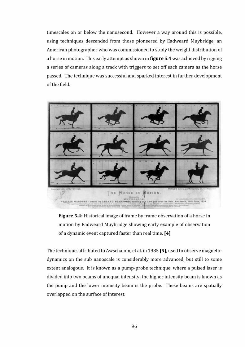
96
timescales on or below the nanosecond. However a way around this is possible,
using techniques descended from those pioneered by Eadweard Muybridge, an
American photographer who was commissioned to study the weight distribution of
a horse in motion. This early attempt as shown in figure 5.4 was achieved by rigging
a series of cameras along a track with triggers to set off each camera as the horse
passed. The technique was successful and sparked interest in further development
of the field.
Figure 5.4: Historical image of frame by frame observation of a horse in
motion by Eadweard Muybridge showing early example of observation
of a dynamic event captured faster than real time. [4]
The technique, attributed to Awschalom, et al. in 1985 [5], used to observe magneto-
dynamics on the sub nanoscale is considerably more advanced, but still to some
extent analogous. It is known as a pump-probe technique, where a pulsed laser is
divided into two beams of unequal intensity; the higher intensity beam is known as
the pump and the lower intensity beam is the probe. These beams are spatially
overlapped on the surface of interest.

97
Temporal resolution is achieved by varying the travel length, and thus the phase of
one beam with respect to the other. In the analogy, if the horse was running on the
spot and a single camera was used with a variable trigger, you could build up a
picture of the dynamics over the course of many ‘runs’. The important point to bear
in mind here is that over the course of the experiment, any movements that were
not repeatable would be blurred out and lost and only repeatable dynamics would
be visible. So it is with pump-probe magneto-optics, the data captured represents
the change and resetting of the dynamics, probably many thousands of times. In this
manner it is important to bear in mind that the repetition rate of the observation
system (laser pulse) must be significantly slower than the duration of the event
(magnetic dynamics), so that each repetition finds a completely reset system.
5.3.2 Femtosecond Laser Operation
The femtosecond pulsed laser referred to in this work is a Spectra-Physics Femto
Spitfire system, comprised of three units and configured as shown in figure 5.5:
Figure 5.5: Schematic showing the combination of laser instruments to
form the high-power, short-rise pulsed laser essential to this
investigation.

98
● 21W 527nm diode-pumped, 1kHz Q-switched, Intra-cavity doubled Nd:YLF
Pump Laser ‘Evolution-30’. [6]
● 1.5W 800nm diode-pumped, 1MHz mode-locked Ti:Sapphire Seed Laser ‘Mai-
Tai’. [7]
● 2W Ti:Sapphire 800nm Regenerative Amplifier ‘Spitfire’. [8]
Pump Laser
The Evolution has an output wavelength of 527 nm and uses an array of twelve
AlGaAs laser diodes to excite its Nd:LiYF4 gain medium at 1053 nm. This medium is
chosen for its high thermal conductivity and natural birefringence making it a stable
medium for high pulse energy, low frequency lasers. The narrowband emission of
laser diodes makes them efficient compared to more traditional broadband arc-
lamp sources, which produce extra undesired thermal effects such as depolarization
and thermal lensing. The laser resonator is acousto-optically Q-switched at 1 kHz
with pulses lasting 100 ns. The Q-switching is achieved by periodically propagating
an ultrasonic wave through an optically transparent material (sometimes known as
a Bragg cell), manipulating its optical refractive index through the photo-elastic
effect to periodically deflect a portion of the beam energy out of the cavity. While
the ultrasound is applied, the Q (quality) factor is significantly reduced and lasing is
interrupted. During the intervals, the gain medium is rapidly saturated again,
producing a high Q-factor and restarting lasing, resulting in high energy pulses.
Finally an intra-cavity frequency-doubling (also known as 2nd-harmonic generating
(SHG)) Lithium Triborate (LBO) crystal is used to double the pulse energy by halving
the wavelength to 527 nm output. The output mirror is selected to be 100%
reflective for the fundamental wavelength (1053 nm) and partially transmitting at
the 2nd-harmonic (527 nm), so as to output only the higher energy photons.
Seed Laser
The Mai-Tai seed laser is comprised of a continuous wave (CW) pumping chamber
followed by a pulsed conversion chamber. The first chamber features a diode-

99
pumped, intra-cavity, frequency-doubled, solid-state Nd:YVO4 523 nm laser. The
second chamber is a mode-locked (Titanium) Ti:Sapphire cavity.
The pumping chamber uses a diode laser to pump Neodymium (Nd3+) ions doped in
an Yttrium Vanadate (YVO4) gain crystal. At normal operating temperature, the most
likely emission is at 1064 nm, which is then selected with optics. This wavelength
is then converted to visible light by interaction with a non-linear frequency-
doubling LBO crystal, which is temperature regulated. The output power of this
2nd-harmonic (P2ω) is given by the following:
P2ω ∝ (deff2 Pω
2l2[Φ])/ A (5.1)
Equation 5.1 contains deff the effective nonlinear coefficient, Pω the power of the
fundamental input frequency, l the effective length of the SHG medium, [ϕ] a phase-
matching factor and A representing the cross-sectional area presented by the beam.
As the output power depends on the square of the input power, this is maximised
here by positioning the SHG inside the laser cavity. The pump chamber outputs a
green 532 nm beam and achieves high power stability through the superposition of
many longitudinal laser modes averaging out the effect of ‘beating’.
The second (pulsing) chamber is a long cavity using an active acousto-optic
modulator (AOM) to mode-lock the laser beam and amplify it with a Ti:Sapphire gain
medium. This process shares some small similarities with Q-switching, both
involving the interference of an acoustic wave with an optically transparent
medium. A standing wave is produced in the AOM resulting in a time varying
refractive index grating perpendicular to the beam propagation. A fixed phase
relationship is produced between the propagating laser modes by synchronising the
frequency of this acoustic wave, ωmL, with the frequency of the laser repetition rate
c/2L, where L is the cavity length. It can then be seen that light which is initially in
phase with ωmL will continue to be in phase as it round trips the cavity and is
progressively amplified, while out of phase light will be deflected. This produces a
time varying loss building modulation sidebands which progressively lock
subsequent longitudinal modes in phase with one another. Once in phase these
100
modes, periodically, constructively interfere producing a rapid pulse whose
duration is dependent on the bandwidth of locked modes and can produce pulses
with rise time and falloff on the order of femtoseconds.
Regenerative Amplifier
The Spitfire system employs a state-of-the-art ‘chirped pulse amplification’ (CPA)
technique, pioneered by Mourour & Strickland (1985) [9] to circumvent the
maximum energy limitations in solid-state amplifiers due to the optical damage
threshold (for Ti:Sapphire this is <10 GW/cm2). As shown in figure 5.6, the seed
pulse is temporally stretched prior to entering the amplifying cavity, reducing its
peak power. This is achieved by multiple passes through a pair of optical gratings
such that the pulse experiences a frequency-dependent path length gradient,
drawing its duration out by a factor of 103 or more. This is known as group velocity
dispersion (GVD) or chirp.
The Ti:Sapphire amplifier crystal is excited to population inversion by the pump
laser pulse allowing the stretched seed laser pulse to initiate stimulated emission,
amplifying its energy without changing its wavelength profile. A seed pulse is
selectively retained within the amplifier with a pair of Pockels cells, electro-optical
‘voltage-controlled waveplates’, reducing the repetition rate of the output by a factor
of 103 to concentrate the energy per pulse. Under an appropriately applied voltage
these Pockels cells rotate the beam polarization by precisely 90° per pass, and
otherwise allow the beam to pass unaffected.

101
Figure 5.6: The seed pulse is stretched, reducing its peak power, before
amplification and then recompressed to form a short, high power pulse.
This allows greater amplification circumventing the power damage
threshold of the amplifier.
Figure 5.7: Amplifier regeneration profile observed on oscilloscope. Just
the input Pockels cell activated (left) and the output Pockels additionally
activated (right). This shows an example of a well-tuned regeneration,
points of note: low background interference, sharp build-up, output
timing set to output high pulse power.
In the Spitfire system, these devices are controlled by a Synchronisation and Delay
Generator (SDG II) controller, which is synchronised to an output square wave from
the MaiTai and only active when the seed is reliably mode-locking. The first cell is

102
timed to capture a single seed pulse which can pass 20 or more times through the
cavity before saturating the gain medium, the second cell is timed to eject this pulse
as after that saturating pass. This was tuned by observing a photodiode within the
amplifier and adjusting the relative timing so that the last visible pulse was the
highest energy as demonstrated in figure 5.7.
Maintenance
Careful maintenance of this system is crucial for maximising the signal-to-noise ratio
of any measurements and can save hours on each measurement. As demonstrated
in figure 5.8, below, the stability of the output energy can be affected significantly if
the laser is not operating correctly. This has particularly been attributed to the seed
laser stability.
Figure 5.8: Example of effect of laser stability noise on the detector
output shown on oscilloscope for an unstable situation (left) and after
optimizing (right). Showing signal from detector 1 (top trace), inverted
signal from detector 2 (bottom trace) and the optimized difference
between the channels (middle trace).
While the MaiTai is a closed system designed to inhibit dust ingress its mode-locking
capability still degrades with time, and this can be temporarily offset by manually

103
increasing the output power. This is a method of diminishing returns however and
eventually thorough cleaning of key mirrors and windows is necessary.
5.3.3 Optics Design Process
The experimental set-up went through a number of iterations during the course of
this project, investigating the pros and cons of various configurations. While some
of this will be detailed here, this section will focus on the ultimate design, detailed
in figure 5.9. When setting up the pump-probe instrument, the major points to bear
in mind were as follows:
● The pump beam path length is varied relative to the probe by way of a delay
line of 300 mm (2 ns round trip).
● The pump and probe beam paths are equalized to towards the start of the
delay line - to maximize the post overlap time.
● The delay line is well aligned to minimize any spatial overlap drift between
the beam spots on the sample.
● The beam spots are overlapped with the aid of a webcam and lens system.
● The reflected probe is directed into the detector and any other light is
rejected.

104
Figure 5.9: Schematic of the ultimate experimental set-up used in this
investigation. The laser output is split into transmitted pump (92%) and
reflected probe (8%) by a beam-splitter. The pump beam (red) passes
through a delay line, optical chopper and beam reducer before being
focused onto the sample. The probe (blue) passes through a BBO
wavelength doubling crystal and a polarizer before being focused onto
the sample.
Delay Line
The femtosecond laser was first attenuated to 120 mW and split 92:8 to produce
pump and probe beams. The pump path was then aligned down one side of the delay
line with an x-translation stage, a rotatable mirror and a pinhole (see figure 5.10).

105
This was a very effective method for making sure that the beam was aligned with
the translation path of the delay line in both horizontal and vertical axes
independently. The delay line was a stepper motor driven screw-thread based
translation stage with a full travel of 300 mm and a step resolution of 2.5 µm
corresponding to 16.7 fs.
Figure 5.10: Alignment of the delay line. A pinhole is mounted on the
delay line during alignment to measure the relative deviation in the
beam. A one axis translation stage and rotation mount are used to adjust
the beam entering the delay line to minimize this deviation.
The beam was then redirected back along the delay line, parallel to the incoming
beam. Originally this was achieved with a pair of mirrors set at right angles to each
other, using a similar method of shifting a pinhole and adjusting the mirror tilt to
minimize any deviation. It became clear however later that this alignment left the
system very sensitive to minor unevenness in the delay line itself, making it
impractical when exaggerated through the rest of the system. The effect of this is
demonstrated in figure 5.11 below, which shows a frame by frame observation of
the pump spot position on the sample surface as the delay line travels from start to
end. Linear drift in the spot position can be corrected for, but a non-linear drift was
observed. The alternative was to use a trihedral ‘retroreflector’ prism (corner cube)
which employs total internal reflection to return the beam, parallel to the incident,
to within 14 μrad. This effectively removed any drift caused by delay line
unevenness. With a retroreflector the trajectory of the reflected beam is shifted
unless it is directed at the centre of the prism. This can be dealt with independently

106
for the vertical and horizontal axes and in fact this is a useful property for the
horizontal axis, but had to be carefully corrected for in the vertical axis.
Figure 5.11: Frame-by-frame camera capture of the pump beam spot on
the sample during a delay line movement using two mirrors. Shows a
non-linear drift as the delay line is moved from one end to the other. This
is caused by sub-micron unevenness in the delay line tilting the mirrors.
Beam Overlap
It was critical that the beams should be spatially overlapped on the sample, a non-
trivial matter due to the small margin of error (<1 μm). Initially, the experiment was
set up with a separate lens for the pump beam set normal to the sample surface. A
CCD camera placed in the pump path was unable to detect the probe beam spot, and
when placed in the probe path the true position of the pump beam spot was
obscured. This was discovered by increasing the pump fluence to the point of
burning the sample, which left a mark consistently a few microns to the left of the
apparent position. This resulted in a setup redesign to bring the incident pump
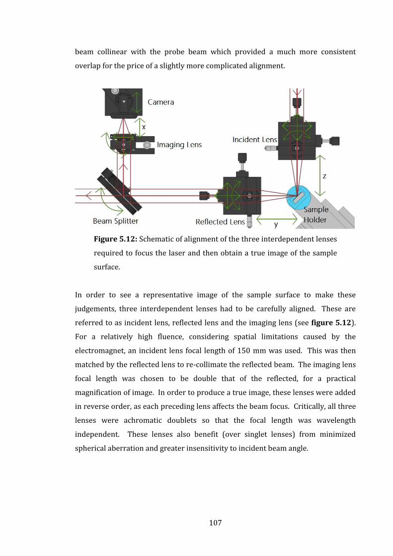
107
beam collinear with the probe beam which provided a much more consistent
overlap for the price of a slightly more complicated alignment.
Figure 5.12: Schematic of alignment of the three interdependent lenses
required to focus the laser and then obtain a true image of the sample
surface.
In order to see a representative image of the sample surface to make these
judgements, three interdependent lenses had to be carefully aligned. These are
referred to as incident lens, reflected lens and the imaging lens (see figure 5.12).
For a relatively high fluence, considering spatial limitations caused by the
electromagnet, an incident lens focal length of 150 mm was used. This was then
matched by the reflected lens to re-collimate the reflected beam. The imaging lens
focal length was chosen to be double that of the reflected, for a practical
magnification of image. In order to produce a true image, these lenses were added
in reverse order, as each preceding lens affects the beam focus. Critically, all three
lenses were achromatic doublets so that the focal length was wavelength
independent. These lenses also benefit (over singlet lenses) from minimized
spherical aberration and greater insensitivity to incident beam angle.

108
Figure 5.13: Camera images of alignment of the three interdependent
lenses required to observe the sample surface clearly. The image lens is
added and moved to focus (left); the reflected lens is added and moved
until a wide-field image of the sample surface is in focus (middle); the
incident lens is added and moved until the beam focus is observed again.
This is done for both pump and probe together and overlapped (right).
1. The pump and probe beams were aligned parallel, to within 2 mm over 6 m (0.3
mrad).
2. With no lenses inserted, the two laser beams were directed at 45° onto the
sample surface and reflected off towards the detector (which was positioned
based on this beam line).
3. 8% of the beam was split off at 90° and onto the camera CCD active area, centred
with the live image feed - at this point, the image was of the illuminated sample
surface.
4. The imaging lens was inserted and aligned so that distance x is the image lens
focal length - the image became beam spots and focus was found by tuning until
diffraction spots were observable from both pump and probe beams (see figure
5.13).
5. After next inserting the reflected lens, its position was adjusted until distance y
was equal to its focal length whereupon the image once again becomes that of
the illuminated sample surface.
109
6. Finally the incident lens was inserted and positioned so that z equalled its focal
length - the image is now again of the pump and probe spots and any deviation
in their paths could be observed and corrected for.
At this point a true image of the position and focus of the beam spots was observable
and fine alignment of the delay line and overlap was possible.
Beam conditioning
As the pump beam was many times more intense than the probe, it was necessary
to selectively inhibit it from the detector, which was achieved by wavelength
doubling the probe beam after the beam splitter. A barium borate (BBO) crystal,
which has a strong negative uniaxial birefringence, was used as an SHG to drop the
wavelength of the pump beam from 800 nm to 400 nm. A 400 nm narrowband filter
was placed after the BBO crystal and directly before the detector, so that all probe
energy was at 400 (±2) nm and no other light source contributed to a measurement.
In addition a beam block was inserted to catch the reflected pump beam prior to the
detector filter. By intermittently manually blocking the incident probe beam, it was
possible to observe the background intensity picked up by the detector to ensure no
pump was being detected.
Considering the collimated laser beam geometrically, an approximate laser beam
spot radius after focusing, r2 can be related to the initial beam radius r1, its
divergence θd1 (in radians) and the focal length, f of the focal lens [10]. This is shown
schematically in figure 5.14 and equation 5.2.

110
Figure 5.14: Ray diagram of geometry for approximating beam focus
diameter based on lens focal length, f, and incoming beam divergence, θd1
from a collimated beam.
𝐫𝟐 = 𝐟𝛉𝐝𝟏 (5.2)
By setting the focal length as a constant for both pump and probe beams, the relative
radii of the beam spots was altered by increasing the divergence of the pump beam.
This was achieved using a 5x beam reducer placed in the pump beamline, which has
a directly proportional effect on the resultant beam divergence via the following
relationship from a collimated state (equation 5.3) and shown schematically in
figure 5.15.
Figure 5.15: Ray diagram of geometry for calculating change in beam
radius and divergence from a collimated beam.

111
θd2 = θd1 f2/|−f1| (5.3)
Beam power was then converted to fluence (equation 5.4) for a more physically
meaningful measure of the energy associated with the pump beam. This is provided
by the following straightforward relationship, and is quoted here in µJ/cm2.
Fluence = Laser pulse energy / Effective focal spot area (5.4)
5.3.4 Signal Capture & Electronic Considerations
As the signal strength is very low in TRMOKE experiments of this type (especially in
the longitudinal configuration), maximizing the signal-to-noise ratio (SNR) is very
important. This was achieved by a combination of techniques detailed here.
All coaxial cables used to transfer data were double shielded to minimize electrical
interference and a two detector bridge configuration was used to eliminate thermal
signal drift. Before each measurement, the signal from the detectors was first routed
through a fast response (1 MHz) digital oscilloscope to evaluate the signal. At this
point, the Pockels cells timings, probe intensity, background light leakage, detector
balance and temporal overlap were checked.
The signal is then passed through a lock-in amplifier which allows the detection of a
real signal buried within noise, which may be of the same magnitude or even larger
[11]. In order to achieve this, an optical beam chopper is placed in the pump path
to provide an external reference frequency of a few hundred hertz on top of the
experiment’s driving force. This is necessary as the repetition rate of the laser is too
high to be used. The lock-in amplifier then employs a technique known as phase-
sensitive detection (PSD) to selectively respond only to the signal which occurs at
that reference frequency with a fixed phase relationship. This acts like a very
narrow bandpass filter centred on the external reference frequency. The lock-in
produces its own internal reference signal (equation 5.5), with an amplitude VL,
frequency ωL and locked to Θref the phase of the external reference. The input signal

112
(equation 5.6) is amplified and multiplied by the reference frequency to produce
two AC signals (equation 5.7), one at the difference frequency (ωsig − ωL), and one
at the sum (ωsig + ωL). The highly desirable DC signal, VDC, is then extracted using
a low pass filter to form the lock-in output (equation 5.8), proportional to the
amplitude of the input signal.
Internal reference signal = VLsin(ωLt + Θref) (5.5)
Input signal = Vsigsin(ωsigt + Θsig) (5.6)
VAC = ½VsigVLcos[(ωsig − ωL)t + Θsig − Θref] (5.7)
−½VsigVLcos[(ωsig + ωL)t + Θsig + Θref]
VDC = ½VsigVLcos(Θsig − Θref) (5.8)
With the delay line set to a point after the pump-probe temporal overlap, it is
possible to observe the signal quality directly from the lock-in. The low pass filter
was chosen to have a time constant (TC) no longer than necessary, which was
judged, by preliminary measurements, to be in the region of 2 seconds as an
acceptable compromise of speed and accuracy. This was dependent on the stability
of the laser and quality of alignment. This filter then essentially averaged the
response from 20,000 pump events to form the output. Finally the lock-in gain was
increased until the signal filled approximately 40% of the dynamic range (~20-100
dB) which left sufficient room for larger signals.
From this point, the signal was passed via a high performance Data Acquisition NI-
DAQ card to LabVIEW software to be recorded. Further SNR improvements were
necessary by averaging the result of a large number of demagnetization events. In
order to achieve an acceptable signal-to-noise ratio (>20) it was necessary to
average each time delay point for at least 30 seconds, in addition to allowing a 4 ×TC
settling time (8 seconds) after any change of the delay line to avoid blurring of the

113
signal. Optimizing the SNR could save hours on a complete measurement which
generally consisted of >300 data points.
5.3.5 Design of Software
LabVIEW software was created to run the TRMOKE experiments. This programme
was designed to be modular and was improved and added to regularly by the author
over the course of the project. The programme was built using a state machine
structure. As the magneto-dynamics occur over a number of vastly different
timescales throughout the experiment, the programme was constructed with a
settings menu (figure 5.17) which allowed the delay line time array to be set to five
different step sizes, and could be set by mm or ps. An electromagnet set-up was
added to allow for dynamic hysteresis loops and multiple runs over a series of
external field strength to be produced.
In order to standardize the measurement documentation, a set of experimental
protocols were produced, requiring the user to go through a check-list of
parameters prior to initializing an experiment (figure 5.19). This improved record
keeping between group members and ensured a comprehensive list of parameters
exist for each experiment.
This was particularly important for the lock-in parameters as this information
repeatedly became relevant weeks or more after a measurement had been taken.
Software settings were automatically imported into the parameter save file and save
file and folder names were generated procedurally to maintain a consistent
recording style.

114
Figure 5.16: LabVIEW software front panel, designed to show a number
of useful values such as the applied field strength and runtime
information.
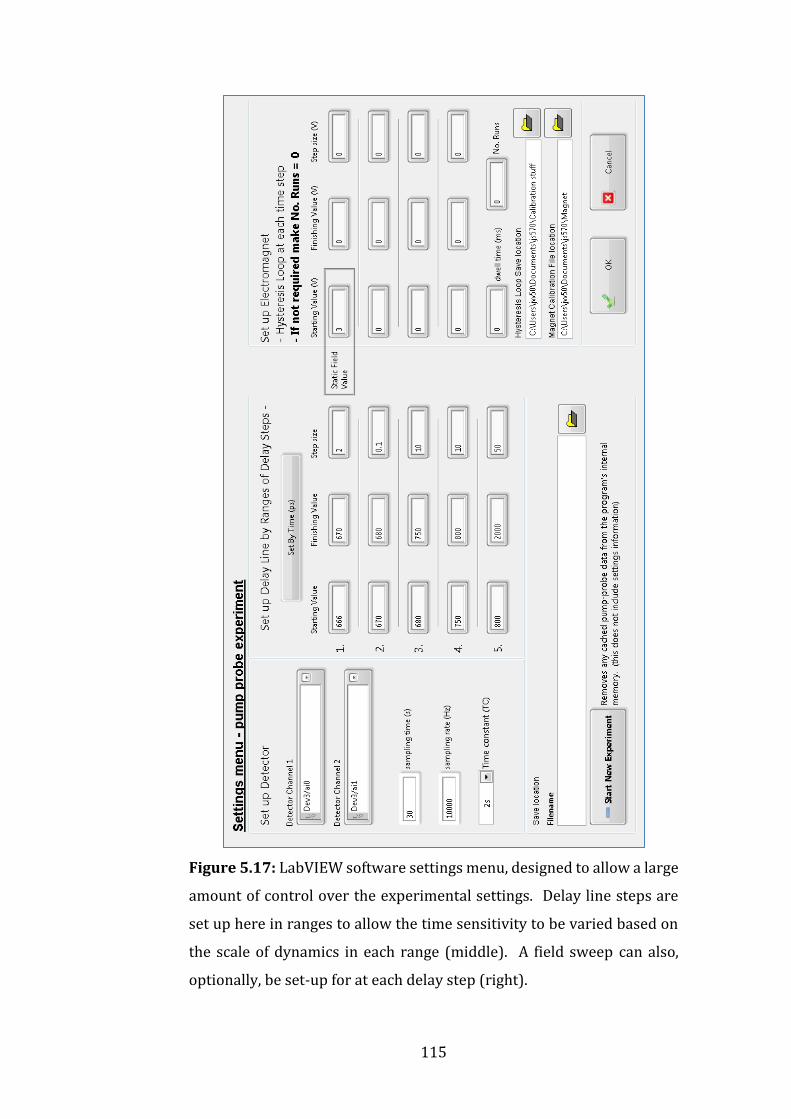
115
Figure 5.17: LabVIEW software settings menu, designed to allow a large
amount of control over the experimental settings. Delay line steps are
set up here in ranges to allow the time sensitivity to be varied based on
the scale of dynamics in each range (middle). A field sweep can also,
optionally, be set-up for at each delay step (right).

116
Figure 5.18: Image showing LabVIEW main experiment ‘For loop’.

117
Figure 5.19: LabVIEW software pre-run information. Each run is saved
with a data sheet containing the useful experimental information and
save filenames and folders are then procedurally generated.
5.4 References
[1] P. N. Argyres, Phys. Rev., 97, 334 (1955)
[2] J. Stöhr, H. C. Siegmann, Magnetism, (Solid-State Sciences Springer Verlag, Berlin,
2006)
[3] C. Bunce, Magnetization Dynamics in Thin-films, (Ph.D Thesis, University of York,
2008)

118
[4] Collections of University of Pennsylvania Archives
[5] D. D. Awschalom, et al., Phys. Rev. Lett., 55, 1128 (1985)
[6] Spectra-Physics Evolution-30 (User Manual, 2003)
[7] Spectra-Physics Mai Tai (User’s Manual, 2002)
[8] Spectra-Physics Spitfire (User’s Manual, 2004)
[9] D. Strickland and G. Mourou, Optics Comm. 56, 219 (1985)
[10] M. Born and E. Wolf, Principles of Optics: Electromagnetic Theory of
Propagation, Interference and Diffraction of Light (Pergamon Press, 1959)
[11] About Lock-In Amplifiers (Stanford Research Systems)
http://www.thinksrs.com/downloads/PDFs/ApplicationNotes/AboutLIAs.pdf

119
Chapter 6
Materials Study of Post-Oxidized Magnetite Thin-Films
6.1 Introduction
Half-metals have been cited as a valuable asset to the field of spintronics for a
number of years, due to the potential improvements to spin transport densities
afforded by 100% spin polarization within the conduction band. Magnetite (Fe3O4)
in particular is considered a promising material for room temperature device
function because of its high Curie temperature (~848 K) [1] and relatively low
coercivity. It is a cheap, commonly available ferrimagnet which forms an inverse
spinel structure with a high lattice matchup to other oxide formations, such as the
insulator magnesium oxide (MgO) appropriate for producing a tunnelling barrier.
The roadblock to large-scale adoption falls with the difficulty of producing and
controlling the properties of high quality thin-films, especially the density and type
of anti-domain phase boundary (APB) defects.
This chapter will discuss growth of epitaxial single crystal magnetite thin-films on
MgO (001) substrate, focusing on identification and characterisation after growth.
The tiny mismatch of ~0.3%, between the relaxed lattice of the film and substrate,
120
means MgO (001) is an excellent template on which to discuss magnetite growth
relatively independently.
6.2 Experimental
All samples detailed were grown by initial molecular beam epitaxy (MBE)
deposition of an iron film, on an MgO (001) substrate, via e-beam heating of an iron
source at a base pressure of 10−9 mbar and the growth rate was fixed at 0.42
nm/min. This was followed by a period of in-situ exposure to atomic oxygen at an
elevated temperature of 320 °C. A chamber pressure of 5 × 10⁻⁵ mbar was
maintained for the duration of the oxidation. Samples were cooled to room
temperature before removing from vacuum. This was the responsibility of Dr. Chris
Kelley and Dr. Siew Wai Poon, with the assistance of Dr. Ben Murphy and the author.
An initial pair of samples was produced at contrasting oxidation times of 15 minutes
and 60 minutes for initial iron film thicknesses of approximately 3 nm. A third was
also grown, sharing the 15 minute oxidation time, but for an initial iron thickness of
~20 nm. A further set of samples was then grown under the same growth conditions
for thick (20 nm) iron films under a series of oxidation times of 9-45 mins.
Magnetometry data was taken by vibrating sample magnetometry (VSM), a high-
accuracy magnetometry technique which measures the net magnetic response of
the entire sample, including substrate, by oscillating it within a variable magnetic
field and measuring the response. Following this, electron transparent cross-section
samples were prepared by mechanical grinding and argon ion milling. This was
followed by plasma cleaning and optical baking to suppress contamination artefacts.
High resolution transmission electron microscopy (HRTEM) analysis was
undertaken using a JEOL FS-2200 aberration corrected electron microscope and a
JEOL 2011 electron microscope.
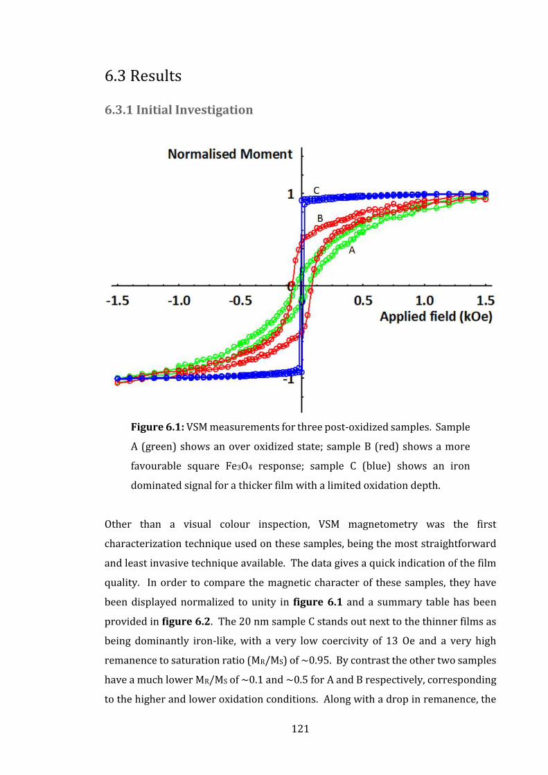
121
6.3 Results
6.3.1 Initial Investigation
Figure 6.1: VSM measurements for three post-oxidized samples. Sample
A (green) shows an over oxidized state; sample B (red) shows a more
favourable square Fe3O4 response; sample C (blue) shows an iron
dominated signal for a thicker film with a limited oxidation depth.
Other than a visual colour inspection, VSM magnetometry was the first
characterization technique used on these samples, being the most straightforward
and least invasive technique available. The data gives a quick indication of the film
quality. In order to compare the magnetic character of these samples, they have
been displayed normalized to unity in figure 6.1 and a summary table has been
provided in figure 6.2. The 20 nm sample C stands out next to the thinner films as
being dominantly iron-like, with a very low coercivity of 13 Oe and a very high
remanence to saturation ratio (MR/MS) of ~0.95. By contrast the other two samples
have a much lower MR/MS of ~0.1 and ~0.5 for A and B respectively, corresponding
to the higher and lower oxidation conditions. Along with a drop in remanence, the

122
increased oxidation also results in a drop in coercivity of 34% from 79 Oe to 51 Oe.
Sample B showed a relatively ordered magnetization reversal and sample A show a
much more disordered reversal.
Absolute values of saturation magnetisation can be useful in characterizing a
material when volume normalized. For samples A, B and C the measured saturations
were respectively 0.00028 emu, 0.0003 emu and 0.002 emu. As each sample was
measured from a 1 x 1 cm substrate wafer, the film volume can be approximated
along with its thickness of approximately 6nm, 6nm, and 20nm. This provides
estimated volume corrected saturations of 467 emu/cc, 500 emu/cc and 1010
emu/cc, respectively.
From literature [2], an iron film is expected to show in the region of 1700 emu/cc,
whereas for a magnetite film it should be close to 480 emu/cc. The inaccuracy
comes in estimating precisely the volume of film present in the measurement, as is
recognised by literature. It would however imply that an uncompensated iron
contribution may still exist within the 15 min sample. Substrate effects have been
removed from these samples, and represent a ~0.01% contribution. Expected value
for coercivity for iron is around 4 Oe and between 30-100 Oe for magnetite. This
data suggests an over-oxidation taking place, where the oxidized film from A to B is
losing coherence and experiencing increased domain wall pinning.
Sample Nominal Thickness (nm)
Oxidation Time (min)
Coercivity, HC (Oe)
Absolute Magnetization MS (emu/cc)
Normalized Remanence MR/MS
A 3 60 51 467 0.1
B 3 15 79 500 0.5
C 20 15 13 1010 0.9
Figure 6.2: Table showing growth and magnetometry information for
thin over-oxidized sample A; thin less oxidized sample B; thick
unoxidized layer-dominated sample C.

123
Figure 6.3: HRTEM cross-section of 15 minutes oxidation time (top) and
60 minutes oxidation time thin samples (bottom). Showing the
substrate, film and vacuum (guide lines have been added to compare
with figure 6.5).
Further investigation of the difference between the oxidation times was performed
by taking a cross-section of the samples in the (100) direction, as is a standard
characterization technique. HRTEM of samples (a) and (b), shown in figure 6.3,
reveal the difficulty in interpreting the magnetization data. Very little difference can
be observed between the two, which both show high quality single crystal spinel
structure with the characteristic 45° planes. Select area diffraction (SADIFF)
5 nm
5 nm

124
imaging of the films, seen in figure 6.4, indicates highly regular spinel structure and
confirms the epitaxial nature of the film to substrate.
Figure 6.4: Select area diffraction of 15 minute oxidation time thin-film
(top left); 60 minute oxidation time thin-film (top middle); MgO
substrate (top right); calculated pattern of Fe3O4 (001) (bottom left) and
MgO (001) (bottom right). Yellow squares mark out common oxygen
sublattice pattern and blue squares mark out Fe3O4 unit cell pattern,
displaying inverse spinel structure.
All SADIFF images were taken on the JEOL 2011 microscope with an electron
wavelength (λ) of 0.0253 Å at a camera length (L) of 500 mm. Using the MgO (001)
substrate diffraction image as a reference, it is possible to check the calibration of
the images using the equation λL = dhklRhkl where dhkl is the distance between
lattice planes and Rhkl is the observed spot spacing on the image. As MgO and Fe3O4
share an oxygen sublattice, the substrate diffraction image appears similar to that of
the film but missing the additional atomic planes formed by the iron sublattice.
Measuring from the 020 to the 020 spots on the image gave a distance of half a unit
cell at 6.006 ±0.005 mm, giving a calculated lattice parameter of 4.212 ±0.003 Å

125
compared to the actual spacing of 4.212 Å. Continuing this analysis for the film gives
an equivalent lattice spacing of 3.014 ±0.005 mm from 220 to 220 which becomes
8.394 ±0.014 Å compared to 8.397 Å in bulk Fe3O4.
The epitaxial relationship between the film and substrate can be shown by
comparing the oxygen sublattice spacing to that of the substrate. For sample A, at
6.001 mm this works out to be 4.216 ±0.04 Å with a 0.9 (±0.8) % lattice mismatch.
Similarly for sample B at 5.998 ±0.005 mm this gives 4.218 ±0.04 Å with a 1.4 (±0.8)
% lattice mismatch. This is evidential of the expected epitaxial relationship, close to
the expected 0.3 % lattice mismatch.
It is possible to further analyze the quality of these films by isolating the {220}
planar contributions to each image, which only exist in the spinel structure. The
result of this is shown in figure 6.5 and gives some limited extra insight into the
level of disorder in the two films. Horizontal lines have been added as a guide to the
eye to indicate where the film||substrate and film||vacuum interfaces occur.
Figure 6.5: Bragg filtered images of (a) 60 minute oxidation time thin-
film and substrate; (b) 15 minute oxidation time thin-film and substrate.
Greater disorder is observable in (a) compared to (b).

126
HRTEM images alongside the Bragg filtered images show that an elevated state of
disorder existed in the sample with increased oxidation time, consistent with
magnetometry. Both samples exhibited one or two atoms roughness on the surface
and both samples also showed some roughness to film||substrate interface, with
intermixing occurring over, again, one or two atomic planes. The disorder in sample
(b) was greater than for sample (a). The third sample (c) was grown much thicker
(~20 nm) so as to investigate the penetration depth of the oxide layer and observe
the oxide||iron and iron||substrate interfaces. As mentioned previously, the
magnetometry revealed that the film was dominated by the iron contribution and
the microscopy corroborated this as shown in figure 6.6 below. The immediate
striking observation was that the oxide/iron interface was almost atomically flat
and that both layers showed long range crystalline order.
Figure 6.6: TEM image showing long range film with sharp interface and
uniform depth (left). Select area diffraction (right) shows Fe3O4 (100),
Fe (110) and MgO (100) crystalline order epitaxially stacked.
Diffraction analysis showed evidence of Fe3O4 (100), MgO (100) and Fe (110)
existing epitaxially together in this arrangement. By resolving the sample, shown in
figure 6.7(a), (c), it was possible to see what could be a ‘freeze-frame’ of the growth
process and how sharp the interface between oxide and iron layers was. Following
the same processing technique used on the previous samples: Bragg filtering just

127
the vertical {200} planes (see figure 6.4 (c)), it was possible to observe the effect of
the lattice mismatching between the three layers (see figure 6.7(b), (d)).
Figure 6.7: HRTEM images of Fe3O4 (100)||Fe (110) interface (far left)
with Bragg filtered image (mid left) and of Fe (110)||MgO (100) interface
(mid right) with corresponding Bragg filtered image (far right). Crystal
plane dislocations are identified from the Bragg filtered images and
circled showing regular predictable mismatch in Fe3O4||Fe, but irregular
mismatch in Fe||MgO.
5 n
m
5 n
m
5 n
m
5 n
m

128
The lattice mismatch between MgO (100) and Fe3O4 (100) is ~0.3% [3], low enough
for strain relaxation to take place without causing many misfit dislocations. The
mismatch between these and Fe (100) however is on the order of 36% [4] and as a
consequence it is unsurprising that the iron film observed was rotated 45° to
produce Fe (110) and a mismatch of ~3.6% to both.
Figure 6.8: Illustrations of the three most common orientations in the
Fe3O4 cubic inverse spinel crystal unit cell. The (110) direction resolves
each atomic column independently, unlike the other two.
High resolution study of the interface between the iron and the iron oxide layers
confirms the sharpness of the transition, which is not atomically sharp but appears
to have completely transitioned after two or three monolayers. It is interesting to
note then that, although the lattice mismatch between MgO (100) and Fe (110) is
approximately equal to that between Fe (110) and Fe3O4 (100), the observed misfit
dislocation periodicity was quite different. It could be argued that the crystallinity
of the substrate will be greater than that of the grown Fe, which would further
suggest that this interface should be more regular; however this was not borne out
in the investigation. The observed Fe (110)||Fe3O4 (100) dislocations occurred
approximately every 15 and 30 planes, which would be consistent with the
mismatch percentage, however the MgO (100)||Fe (110) dislocations occurred
much more randomly. This may be due to differences in the potential strain of each
of these films, and the fact that there is a smaller difference between the Young’s
modulus of Fe and Fe3O4 (2.8%) than between MgO and Fe (14.7%) [5].
(001) (011) (111)

129
Ultimately, the loss of magnetic order is not fully accounted for by the small increase
in disorder observed from the (100) direction microscopy. As previously discussed,
a continuum of oxidation states exists for the iron oxide spinel, based on the state of
the B site iron. The inverse spinel structure, as shown again above in figure 6.8, is
partially obscured in the (100) direction, and also in the (111) direction, which are
the most common orientations observed. This limitation does not exist in the (110)
direction, which might then prove a superior orientation for characterising the film
order.
6.3.2 (110) Microscopy Investigation
A set of samples was grown following the same growth conditions as above, again
varying the post growth oxidation time, but all with thick initial iron growth. These
samples were oxidised for 9, 27 and 45 minutes. Magnetometry of these samples
was inconclusive because of the large iron signal dominating any effect from the
oxide layer. For this set, cross-section sample preparation was performed at 45° to
the wafer orientation, to view the (110) direction. High resolution TEM images for
these samples are shown below in figures 6.9, 6.10. (Images courtesy of Dr. Daniel
Gilks)
Figure 6.9: (110) direction HRTEM of (a) 9 minutes post-oxidized
sample, showing Fe (100), Fe3O4 (110) and substrate. Interface
transition takes place over ~5 monolayers.
2 nm
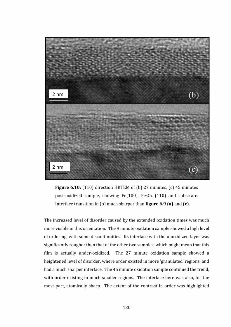
130
Figure 6.10: (110) direction HRTEM of (b) 27 minutes, (c) 45 minutes
post-oxidized sample, showing Fe(100), Fe3O4 (110) and substrate.
Interface transition in (b) much sharper than figure 6.9 (a) and (c).
The increased level of disorder caused by the extended oxidation times was much
more visible in this orientation. The 9 minute oxidation sample showed a high level
of ordering, with some discontinuities. Its interface with the unoxidized layer was
significantly rougher than that of the other two samples, which might mean that this
film is actually under-oxidized. The 27 minute oxidation sample showed a
heightened level of disorder, where order existed in more ‘granulated’ regions, and
had a much sharper interface. The 45 minute oxidation sample continued the trend,
with order existing in much smaller regions. The interface here was also, for the
most part, atomically sharp. The extent of the contrast in order was highlighted
2 nm
2 nm

131
further by Bragg filtering similarly to that done in figure 6.5; this is shown in figure
6.11 for 9 minutes and 45 minutes.
Figure 6.11: Bragg filtered images of 9 minutes (left) and 45 minutes
(right) samples. Shows increase in disorder with oxidation time more
clearly than figure 6.5.
The average thickness of each film was measured by an intensity line profile
averaged horizontally over 2.5 nm and defined by the distance between the first and
last resolved atomic peak in each profile. An example for the 9 minute sample is
shown in figure 6.12. These averaged thicknesses were measured to be 3.115 ±0.05
nm, 3.395 ±0.05 nm and 3.839 ±0.05 nm in order of increasing oxidation time. The
oxide layer appears to reach a skin-depth, as described by Cabrera-Mott oxidation
[6], between 3-4 nm. Although this skin-depth is dominated by both the oxygen
partial pressure and the temperature [7] it is also minimally dependent on the
oxidation time. The oxide layer appears to nucleate rapidly and any further increase
in film thickness is minimal. This suggests that tuning the film’s oxidation time
could be a method of maximizing the quality output of the film.
2 nm 2 nm
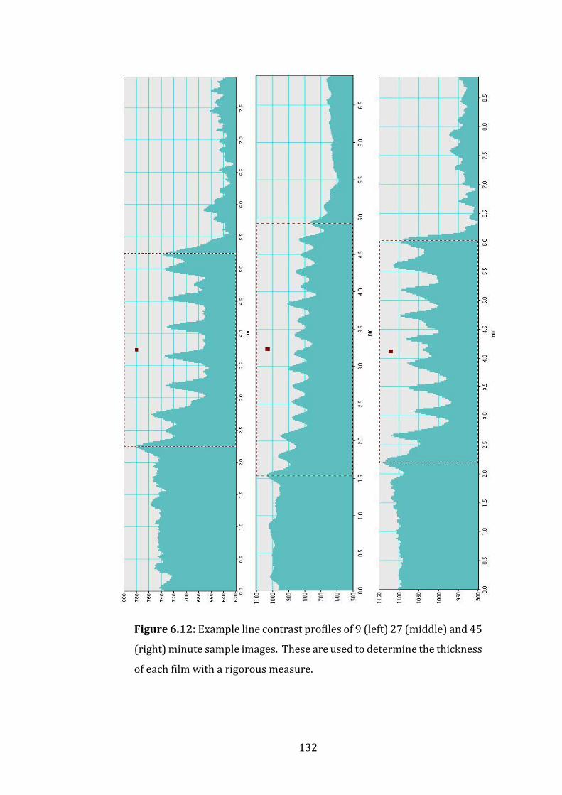
132
Figure 6.12: Example line contrast profiles of 9 (left) 27 (middle) and 45
(right) minute sample images. These are used to determine the thickness
of each film with a rigorous measure.

133
6.3 Fe3O4/MgO(100) APB Geometry
6.3.1 Theoretical Review
An incomplete study of the possible APBs exists for the MgO/Fe3O4 (001) system [8].
In order to properly identify these defects it is necessary to investigate and
catalogue the geometrical non-integer shifts made possible by the relationship
between the MgO (001) surface and the possible terminating planes in magnetite.
This has been carried out to both characterise the APB visibility from experimental
imaging and then to provide geometric data for theoretical calculations of net
superexchange interactions taking place within each system.
Following the work of W. Eerenstein et al. [9] the possible non-integer shifts have
been recalculated for (001) taking the postulate that the magnetite unit cell has
several unique terminating planes. This gives the possibility of more APBs existing
than have previously been reported, without requiring the case of uneven substrate
surface. These defects are reported here along with visibility criteria using the
Howie-Whelan equations.
The magnetite film will lie most naturally with the O sites on top of the Mg sites on
the substrate. This continues the crystal structure with the least disturbance, and is
considered to be the lowest energy state. This work considers a flat MgO surface
termination, with all steps being relative steps in the magnetite unit cell. In
characterising all of the possible non-integer shifts, it is necessary to be aware that
not all geometrically unique shifts are physically unique. It is possible to
characterise a shift which will not tessellate with a second shift, but is essentially
identical and exists as, for example, a mirror image, such as is shown in figure 6.13.
In these cases the listed available superexchange interactions will be the same, and
so one or the other shift can be discounted as trivial.
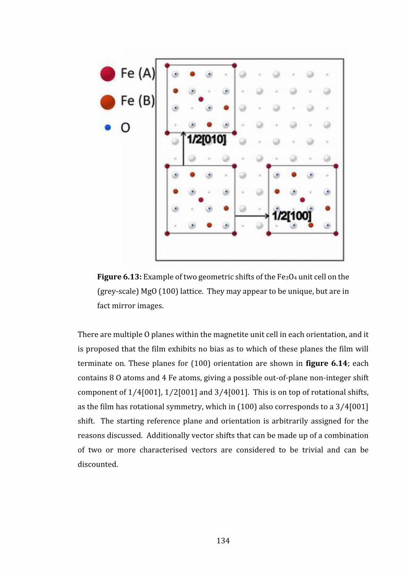
134
Figure 6.13: Example of two geometric shifts of the Fe3O4 unit cell on the
(grey-scale) MgO (100) lattice. They may appear to be unique, but are in
fact mirror images.
There are multiple O planes within the magnetite unit cell in each orientation, and it
is proposed that the film exhibits no bias as to which of these planes the film will
terminate on. These planes for (100) orientation are shown in figure 6.14; each
contains 8 O atoms and 4 Fe atoms, giving a possible out-of-plane non-integer shift
component of 1⁄4[001], 1⁄2[001] and 3⁄4[001]. This is on top of rotational shifts,
as the film has rotational symmetry, which in (100) also corresponds to a 3⁄4[001]
shift. The starting reference plane and orientation is arbitrarily assigned for the
reasons discussed. Additionally vector shifts that can be made up of a combination
of two or more characterised vectors are considered to be trivial and can be
discounted.

135
Figure 6.14: Schematic showing proposed terminating planes of Fe3O4
(100) unit cell. Four octahedral (B) iron atoms exist in each plane,
notably the oxygen lattice is constant through each plane.
Figure 6.15 shows the in-plane shifts. The 1⁄4[-110] and 1⁄4[110] are unique as
they translate over different geometry on the substrate beneath. These have been
previously reported by Eerenstein et al. These shifts will be invisible from a plan-
view of the film. Figures 6.16, 6.17 and 6.18 show the out-of-plane-shifts produced
by this geometry, with the breakdown of some of the vectors shown. In-plane shifts,
1⁄4[-110] and 1⁄4[110] for example, are unique as they are shifted over different
geometry of the underlying lattice; one is shifted across a Mg atom, and the other
across an O atom. Things become more complicated when looking at out-of-plane
shifts, and full calculations of the interactions involved would be needed to deduce
how many of these shifts are in-fact unique.
3
4[001]
4
4[001]
0
4[001]
1
4[001]
1
2[001]

136
Figure 6.15: In-plane APBs on Fe3O4 (100).
Figure 6.16: 1⁄2 z-shift out-of-plane APBs on Fe3O4 (100).

137
Figure 6.17: 1⁄4 z-shift out-of-plane APBs on Fe3O4 (100).
Figure 6.18: 3⁄4 z-shift out-of-plane APBs on Fe3O4 (100).

138
Using the Howie-Whelan APB visibility criteria equation, discussed in chapter 4 and
restated here in equation 4.6, it is possible to calculate the visibility conditions for
these shifts for the first zone of diffraction spots; (220)-type and (400)-type. As can
be seen from figure 6.19, approximately half of the identified shifts are observable
under a (220) dark field condition, and none should be observed under a (400) dark
field condition.
2πg. R = (2N + 1)π (4.6)
This condition is approximately the same as for a stacking fault planar defect. In this
equation, g is the diffraction vector of the electron beam, R is the translation vector
of the planar defect as a fraction of the Fe3O4 unit cell size. N indicates visibility of
an APB for a chosen diffraction spot if it is an integer and invisibility otherwise.
Figure 6.19: Non-integer unit cell shifts and visibility criteria, showing
the in-plane shifts (grey) and out-of-plane shifts.

139
6.3.2 Experimental Observation
A brief investigation of a plan-view slide of the 15 minutes post-oxidized sample was
produced by the lift-off method, detailed in chapter 4, and imaged in the 2011 JEOL
TEM. This sample was chosen as the best of the samples grown which had been
oxidized entirely to the substrate. Standard TEM imaging shows a rough surface
with no obvious inhomogeneity (figure 6.20 right), however diffraction imaging
(figure 6.20 left) shows an extra crystal structure overlaid on top of the inverse
spinel of the Fe3O4. On inspection this is a signal from gamma-phase Fe2O3
maghemite.
Figure 6.20: Images showing example diffraction pattern for 15mins
sample (top left); a TEM image of the sample surface (top right);
calculated gamma-phase Fe2O3 maghemite, observed in plan-view
analysis (bottom left) and calculated Fe3O4 diffraction pattern (bottom
right).
40 nm

140
Dark field image observations were made under the two beam condition to increase
image contrast. Images were taken of the APBs observed, isolating a (220) and
(400) spot individually (see figure 6.21, 6.22).
APBs are clearly visible in figure 6.21 which shows the sample in plan-view looking
in the (001) direction under the [220] dark field condition. The defect density is
surprisingly high considering the quality of the cross-section information. They
appear to be restricted in their direction of propagation in a way that was not
apparent in W. Eerenstein’s [9] simultaneously oxidized films. This disorder will
cause the reduced quality of the magnetic response.
Figure 6.21: Images showing plane-view TEM images of two regions of
15 minute post-oxidized film under [220] dark field conditions which
show a large defect density.
20 nm 20 nm

141
Figure 6.22: Images showing plane-view TEM images of 15 minute post-
oxidized film under [400] dark field conditions, showing visible defects,
as well as Moiré fringes.
Isolating the area around a [400] spot in the post-oxidised film gave images such as
figure 6.22. As these films have maghemite signal in plan-view, this dark field image
also contains contributions from the [130] type spot which is very close to the [400]
as seen in figure 6.20. This observation is interesting firstly because it contains
APBs, when this spot is considered to highlight none. These are potentially due to
the contribution of the maghemite spot making more defects visible. The fringe
patterns in this image are the second point of interest. These are too widely spaced
to be atomic planes and are in fact Moiré interference patterns [10], observed when
two lattices of differing period or orientation interfere with each other. This is a
further indication that there is a surface layer of over-oxidised iron on this film, not
20 nm
142
present in the cross-section and is likely due to the instability of the film surface to
further oxidation during the lift-off process.
6.4 Summary
A pair of Fe3O4||MgO (001) samples have been grown by MBE by post-oxidizing 3
nm thin-films of epitaxial Fe. Increased oxidation time from 15 minutes to 60
minutes has shown a significant reduction in magnetic quality metrics of coercivity
(~35%) and remanence (~80%). Investigation of the crystal structure by cross-
section HRTEM in the standard (001) direction has shown the difficulty of
identifying any increased film disorder and would suggest both films are of
equivalent quality.
Further investigation of a series of 9, 27 and 45 minutes post-oxidized samples has
shown that the disorder exists on the B site Fe ions in the lattice, by HRTEM
observation in the (011) direction. This disorder is strongly dependent on the
oxidation time, while the inverse spinel structure is more robust than expected.
20 nm Fe films, post-oxidized for 9, 27 and 45 minutes show a skin depth to the
oxidation, of 3-4 nm for the chosen temperature and pressure. This was seen to be
only very weakly dependent on oxidation time.
By taking another look at the geometry of the magnetite unit cell, a number of
potential extra APB defects have been identified. Looking at the layers of the unit
cell in the given orientation, it was theorized that a number of unique surfaces
existed on which the film could terminate. As the growth conditions presume island
growth, this could lead to z-shifts between neighbouring islands of Fe3O4 previously
unappreciated in the literature.
As the visibility criteria suggest that approximately half of the shifts are viewable in
plan-view, the actual density can be approximated from experimental data as being
twice that observed. It is interesting that the defects appear to be clearly grouped

143
based on their z-shift component, despite it having no direct contribution to the
calculation for either [220] or [400] vectors.
APBs have been experimentally observed under both spot conditions. It has been
seen that even the 15 minute post-oxidized sample contains a dense APB network,
which explains the undesired reduction in remanent magnetization from an ideal
square loop.
6.5 References
[1] Vescovo et al., J. Appl. Phys., 98, 084507 (2005)
[2] Y. Cao, et al., J. Magn. Magn. Mat. 395, 361 (2015)
[2] R. J. Beals, et al., J. Am. Ceram. Soc., 40, 279 (1957)
[3] W. Zhong, et al., Phys. Rev. B, 47, 95 (1993)
[4] H. M. Ledbetter and R. P. Reed, J. Phys. Chem. Ref. Data, 2, 531 (1973)
[5] N. Cabrera and N. F. Mott, Rep. Prog. Phys., 12, 163 (1949)
[6] T-M Lu et al. J. Appl. Phys., 95, 4346 (2004)
[7] S. K. Arora, J. Appl. Phys., 100, 073908 (2006)
[8] W. Eerenstein, et al. Eur. Phys. J. B., 36, 271 (2003)
[9] D. B. Williams and C. B. Carter, Transmission Electron Microscopy: II Diffraction
(Plenum Press, New York, 1996)

144
Chapter 7
Ultrafast Magnetization Dynamics Study of GdFe Thin-Films
7.1 Introduction
As discussed previously in chapter 3, rare-earth transition-metal alloys (RE-TM),
including GdFe, have been of interest to industrial and commercial applications for
decades [1]. It is as exciting today with the development of new non-volatile, high
density, fast access devices under the umbrella of magnetic random access memory
(MRAM). They are important because of the interaction between their two
sublattices giving these materials the desirable extreme stability and high magnetic
anisotropy under operating conditions. Data recording is required to reach
frequencies into the GHz regime and beyond and field pulsed techniques are
physically limited to the tens of picoseconds. The development of ultrafast pulsed
laser systems since 1996 has opened up new avenues of exploration into methods
of manipulating and observing the dynamic behaviour of these magnetic materials
and, despite high levels of interest, the underlying mechanisms are still the subject
of significant debate [2]. Ultrafast laser stimuli have been applied to explore
coherent spin precession without using a pulsed magnetic field. The ability to
carefully control the spin state of a magnetic material through optical interaction
could have a significant impact on the world of micro/nano-electronics [3]. Further
research is still necessary to understand these interactions with materials.
145
An initial series of GdFe amorphous alloy thin-film samples, of varying Gd
concentration, is studied here by static magnetometry. The focus is to investigate
the temperature dependencies of each. Pump fluence dependent laser-induced
magnetization dynamics is then investigated, in a selected concentration of Gd, using
the time-resolved magneto-optic Kerr effect (TRMOKE) apparatus whose design
and construction is detailed in chapter 5.
7.2 Methodology
Samples used in this investigation were grown by direct current magnetron co-
sputtering onto cleaned Si (001) substrates by collaborators in Nanjing, China using
the Ar gas, magnetron co-sputtering. Details of this procedure are documented in
chapter 4. A series of Gd concentration was produced, with total film thickness of
~20 nm and Gd concentration of 10%-25%. From this set, the 25% Gd
concentration sample was chosen to perform a time-resolved dynamic
measurement investigation.
Laser-induced, pump-probe, room temperature TRMOKE in a longitudinal
configuration was used to optically induce and measure a demagnetization event. A
reference magnetization state was provided by a (>sample coercivity) 1 kOe in-
plane external magnetic field perpendicular to the sample’s magnetic easy axis.
Ultrafast (~100 fs) regenerative Ti:Sapphire laser light with a repetition rate of 1
kHz was used for both pump and probe beams. A central wavelength of 800 nm was
used for the pump beam and 400 nm for the probe. Pump and probe beams were
linearly polarized orthogonal to each other, in s and p orientation respectively, and
both incident to the sample surface at ~45°. The overlap of both beams was
carefully aligned with precision optics and a magnified digital camera image through
a shared focal lens of f=150 mm. A 4x beam reducer was included in the pump beam
to modify the relative spot sizes of pump and probe to improve the overlap margin
of error. Further details can be found in chapter 5. Pump power was varied from
350 µW to 1450 µW, which corresponds to a fluence range of 20 µJ/cm2 to 82
µJ/cm2, over twelve increments. Due to the risk of permanent damage to the

146
measured sample area, the lowest fluence measurement was undertaken first, and
then proceeding from there until saturation was reached.
Note on MOKE measurement calibrations
Values of Kerr rotation and reflectivity are given in internally consistent figures of
voltage linearly proportional to change in magnetization and temperature
(respectively). While it would be ideal to calculate the scaling factors for each, this
is necessarily an empirical process, requiring calibration points for a particular
sample. To calibrate for magnetization requires that the sample is at rest in a
saturated state for the detector balancing, and that a second state of full
demagnetization is recorded under the same laser, lock-in and detector conditions.
This is possible to do by pumping the sample with sufficient fluence as to detect a
full demagnetization without burning the sample. This can be difficult to define
however and an alternative method using a variable electromagnet to detect a state
of fully saturated reversal is better. This author was in the process of establishing
this method during the writing of this document. A reliable temperature calibration
is more complicated still, and would require calibration of reflective surfaces of
know temperatures. This could be done with a cryostat system which is also being
commissioned.
7.3 Results
7.3.1 Static Hysteresis Measurements
Static MOKE measurements at varying in-plane orientations of the sample (figure
7.1) show that it has strong in-plane anisotropy. The in-plane anisotropy tells us
that there is a degree of crystalline order in the sample film, as an amorphous film
would not produce this effect. Additionally as the substrate is diamond cubic
Si(001), a completely epitaxial film would present a four-fold rotational symmetry,
with its hard axis at 45 ׄ° (in-plane) to its easy axis.

147
For the TRMOKE measurements, to stimulate precessional dynamics, it is necessary
to apply the external field along the hard axis, making the resultant change in the
effective field direction as large as possible, increasing the signal strength. An
external field of 1 kOe was chosen to be >>Hc, the coercivity, which was ~25 Oe at
the hard axis.
Figure 7.1: Normalized static MOKE longitudinal hysteresis
measurements showing the anisotropic magneto-optic response. All
TRMOKE measurements are undertaken at the in-plane hard axis, 0°
here.
No
rmal
ized
Ker
r R
ota
tio
n (
M/M
s)
Applied Field (Oe)

148
7.3.2 Pump Fluence Series of Gd0.25Fe0.75
Fluence is an important factor in understanding the behaviour of a material,
especially one as complex as GdFe [4]. From a technological standpoint, the power
requirements of a laser system to perform magnetic manipulation are also critical
for bringing a product to a state of commercial feasibility.
Reflectivity
Time-resolved reflectivity data was produced for the series of twelve pump fluence
measurements from the sum of the detector signal intensities, representing the total
energy reflected from the sample and is proportional to the combined temperature
of the local electron and lattice reservoirs. The noise level was higher in this data
than for the Kerr rotation data detailed later. This is due to the nature of the
measurement technique meaning that instead of negating any laser intensity
fluctuations, they are instead doubled. This does not detract from the
meaningfulness of this data however as the signal-to-noise ratio (SNR) is still >10 at
each peak reflectivity. Slightly higher laser instability was present for the latter,
higher fluence measurements. The reflectivity is seen to consistently increase, over
the course of 2 ps in response to the pump photon injection, independent of fluence.
This initial rise in surface temperature is due to a rapid photon-electron energy
transfer followed by electron-electron thermalization.
The height of the reflectivity peak corresponds to the magnitude of the energy
initially transferred into both the electron and lattice reservoirs and is presented
alongside the equivalent data for the Kerr rotation (which shows the same for the
spin reservoir) in figure 7.2. Errors for both data sets represent the effect of the
instability of the laser hence, as previously mentioned, the Kerr signal data has a
significantly lower average error. The amplitude of the reflectivity peak shows a
significant step at pump fluence between 37-42 µJ/cm2 from a shallow linearly
increasing relationship to a second steeper regime. This second regime appears to
tend towards saturation above ~70 µJ/cm2. By comparison, the amplitude of the
maximum Kerr signal shows no discontinuity, but progresses from a linear regime
to a gradual saturation after ~54 µJ/cm2.

149
Figure 7.2: Amplitude of maximum reflectivity peak (red) compared to
equivalent maximum Kerr signal peak (blue) as a function of pump
fluence.
Figure 7.3: Recovery time constant of the local sample reflectivity, as a
function of pump fluence. Two regimes of energy dissipation are
observed. For low fluence, this is not energy dependent, but for higher
fluence it becomes significantly so.
Pump fluence (µJ/cm2)
Am
pli
tud
e o
f P
eak
Sig
nal
(V
) T
ota
l ele
vate
d t
emp
erat
ure
tim
e (p
s)
Pump fluence (µJ/cm2)
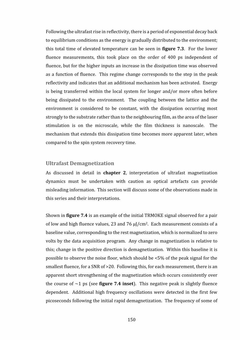
150
Following the ultrafast rise in reflectivity, there is a period of exponential decay back
to equilibrium conditions as the energy is gradually distributed to the environment;
this total time of elevated temperature can be seen in figure 7.3. For the lower
fluence measurements, this took place on the order of 400 ps independent of
fluence, but for the higher inputs an increase in the dissipation time was observed
as a function of fluence. This regime change corresponds to the step in the peak
reflectivity and indicates that an additional mechanism has been activated. Energy
is being transferred within the local system for longer and/or more often before
being dissipated to the environment. The coupling between the lattice and the
environment is considered to be constant, with the dissipation occurring most
strongly to the substrate rather than to the neighbouring film, as the area of the laser
stimulation is on the microscale, while the film thickness is nanoscale. The
mechanism that extends this dissipation time becomes more apparent later, when
compared to the spin system recovery time.
Ultrafast Demagnetization
As discussed in detail in chapter 2, interpretation of ultrafast magnetization
dynamics must be undertaken with caution as optical artefacts can provide
misleading information. This section will discuss some of the observations made in
this series and their interpretations.
Shown in figure 7.4 is an example of the initial TRMOKE signal observed for a pair
of low and high fluence values, 23 and 76 µJ/cm2. Each measurement consists of a
baseline value, corresponding to the rest magnetization, which is normalized to zero
volts by the data acquisition program. Any change in magnetization is relative to
this; change in the positive direction is demagnetization. Within this baseline it is
possible to observe the noise floor, which should be <5% of the peak signal for the
smallest fluence, for a SNR of >20. Following this, for each measurement, there is an
apparent short strengthening of the magnetization which occurs consistently over
the course of ~1 ps (see figure 7.4 inset). This negative peak is slightly fluence
dependent. Additional high frequency oscillations were detected in the first few
picoseconds following the initial rapid demagnetization. The frequency of some of

151
these oscillations are dependent on the data acquisition sampling parameters and
are as such discredited as true signal, however some persistent behaviour is
observable.
Figure 7.4: Graph showing ultrafast demagnetization curves for low (a),
(black), (23 µJ/cm2) and high fluence (b), (red), (76 µJ/cm2). Inset graph
shows the picosecond timescale drop in magnetization and the high
frequency artefacts which affect the regime highlighted in the blue
dashed region.
As discussed in chapter 2, the energy associated with Heff is Eeff = EZee + Eex +
Eani + Edem and each of these energies have associated field vectors which are
balanced at equilibrium but respond at different rates based on the time-energy
correlation, t=h/E. This time scale is dominated by the exchange energy term, Eex.
From chapter 3, the behaviour of GdFe comes from the separate sublattice
dynamics of Fe and Gd, which can be assigned their own distinct Heff vectors. The
(a)
(b)
Ker
r R
ota
tio
n (
V)
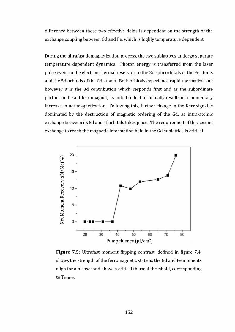
152
difference between these two effective fields is dependent on the strength of the
exchange coupling between Gd and Fe, which is highly temperature dependent.
During the ultrafast demagnetization process, the two sublattices undergo separate
temperature dependent dynamics. Photon energy is transferred from the laser
pulse event to the electron thermal reservoir to the 3d spin orbitals of the Fe atoms
and the 5d orbitals of the Gd atoms. Both orbitals experience rapid thermalization;
however it is the 3d contribution which responds first and as the subordinate
partner in the antiferromagnet, its initial reduction actually results in a momentary
increase in net magnetization. Following this, further change in the Kerr signal is
dominated by the destruction of magnetic ordering of the Gd, as intra-atomic
exchange between its 5d and 4f orbitals takes place. The requirement of this second
exchange to reach the magnetic information held in the Gd sublattice is critical.
Figure 7.5: Ultrafast moment flipping contrast, defined in figure 7.4,
shows the strength of the ferromagnetic state as the Gd and Fe moments
align for a picosecond above a critical thermal threshold, corresponding
to TMcomp.
Pump fluence (µJ/cm2)
Net
Mo
men
t R
eco
very
∆M
/M0
(%
)

153
At lower pump fluences this explanation is simple enough however seen in the
example of 76 µJ/cm2 is again the rapid Fe demagnetization, but this is interrupted
by a short-lived recovery before the second demagnetization phase. This was
observed to occur for all curves above the 37 µJ/cm2 fluence point. The
corresponding height contrast between these turning points, (marked on figure 7.4
as the ultrafast moment flipping differences) is plotted in figure 7.5. A clear phase
transition can be observed above 37 µJ/cm2 which is a point already noted from the
reflectivity data. A transient ferromagnetic state has been theorized, but not
experimentally observed in RE-TM systems such as this. The interpretation of this
behaviour, summarized in figure 7.6, is as follows:
1. Energy is transferred from the electron thermal reservoir to the 3d and 5d spin
orbital thermal reservoirs, which exchange energy with each other to remain
close to equilibrium, but with negligible dissipation to the lattice.
2. The magnetic order associated with the 3d reservoir begins to decay rapidly,
causing a picosecond strengthening of the net magnetic moment.
3. a. The 5d reservoir is also able to exchange energy away to the 4f reservoir and
does so rapidly following the 3d head-start. The large 4f magnetic order begins
to decay and the net magnetic moment reduces rapidly.
b. At some point the 5d and 4f reservoirs reach equilibrium with each other and
the rate of decay of the net magnetic moment slows.
4. If the energy available is sufficient the 3d magnetic moment will reach full
demagnetization and begin to reverse due to conservation of angular
momentum. This results in a momentary ferromagnetic-like alignment of the
magnetic moments causing a short-lived recovery of net moment.
5. The 4f magnetic moment is still decreasing and the net moment begins to fall
again until the net moment reaches a minimum.

154
Figure 7.6: Schematic timeline of the ultrafast magnetic reversal
behaviour.
Figure 7.7: Time for Gd sublattice to reach internal equilibrium, showing
2 critical temperature points (a) and (b).
Pump fluence (µJ/cm2)
0 1 2 3 4 5 6 7 8 9 10 11
Time from laser impulse (ps)
Ker
r R
ota
tio
n (
V)
1 2 3a 4 5
3b
4f Moment
3d Moment
(not to scale) 5d
to
4f
orb
ital
eq
uil
ibri
um
tim
e (p
s)
4
3
2

155
Lastly a fluence dependence was observed in the ultrafast demagnetization time,
defined as the time taken for the 5d and 4f (and therefore 3d and 4f) spin orbitals to
equilibrate (figure 7.7). Below 37 µJ/cm2 this occurs in <1.3 ps, after which a large
increase in the demagnetization time is accounted for by the ferromagnetic
transient state. A second turning point appears around 65 µJ/cm2, after which point
the demagnetization speeds up again. This second turning point is noted and will
be discussed again in relation to further data in the following sections.
Magnetization Recovery Time
Following the ultrafast demagnetization, the recovery of the magnetic order is an
essential observation in understanding the mechanisms at work within any
material. Figures 7.8 and 7.9 show the full time-resolved Kerr rotation signals,
taken simultaneously alongside the reflectivity data; these plots have been y-offset
for clarity.
Figure 7.8: TRMOKE rotation signal as a function of pump fluence for
low pump powers. Oscillatory recovery is observed for each, with the
first oscillation being gradually absorbed into the long range recovery
curve.
42 µJ/cm2
37 µJ/cm2
31 µJ/cm2
25 µJ/cm2
23 µJ/cm2
20 µJ/cm2
Ker
r R
ota
tio
n (
V)
Time (ps)

156
Figure 7.9: TRMOKE rotation signal as a function of pump fluence for
high pump powers. Oscillatory recovery is all but obscured by the long
range recovery curve.
A few observations are immediately apparent: For all low power measurements
(<42 µJ/cm2), after the initial ultrafast demagnetisation, clear coherent oscillations
begin almost immediately. As there is an angle between the external field vector
and the internal anisotropy field vector of this sample, these oscillations are
attributed to the stimulation of damped magnetization precession. A reduction in
the clarity of the oscillations begins to be seen above ~42 µJ/cm2 corresponding to
the point of discontinuity in the reflectivity data; this is despite the maximum signal
height showing no correlation. By the end of the series, these oscillations are almost
completely lost. Along with this loss in amplitude, the start of the precession is
delayed further with increasing fluence as the rate of recovery drops.
In order to calculate the magnetization recovery time, a definition of the starting
point of the recovery was required. This was initially set to the point of maximum
82 µJ/cm2
76 µJ/cm2
71 µJ/cm2
65 µJ/cm2
54 µJ/cm2
48 µJ/cm2
Ker
r R
ota
tio
n (
V)
Time (ps)

157
Kerr signal used to plot figure 7.2, however this did not give a consistent
representation across the series, as the highest fluence plots display an increasingly
broad plateau of stable magnetization (which indicates that the stimulated area of
the sample has reached a full demagnetization condition). This initial setting
distorted later analysis which relied on this measurement, so an alternative
systematic point had to be identified. It was postulated that the beginning of the
recovery was directly linked to a local sample temperature, so by looking at the
higher fluence curves, an approximate point at which the gradient the graph reached
maximum, following the peak signal, was found from derivative calculations. This
required some nuance for the higher fluences as noise and the overlying precession
made a direct automatic calculation inaccurate. This point was found to have a
reasonably consistent correspondence to the time at which the reflectivity data
reached a value of ~4 (arbitrary units representing the voltage from the detector
offset from the reference equilibrium). It is shown on figures 7.7 and 7.8 by the red
circles. This observation then related back to the discontinuity in the reflectivity
data, as the lower fluence measurements did not reach or were on the order of this
value. For the lowest pump fluence curves (20, 23, 25 µJ/cm2) another starting point
was required, which was chosen to be the time delay corresponding to the maximum
reflectivity signal.
For rigorous testing, a second definition of the start of the recovery was also used
(indicated by the blue circles in figures 7.7 and 7.8). This was the point at which
the trend of each curve turned negative. This provided a poorer exponential fit, but
did highlight an extra aspect of the precessional dynamics, which will be detailed
later in this section.
A measure of the magnetization recovery time was then empirically quantified by
fitting an exponential expression Mr(t) = M0 + M1exp(−(t − t0)/τ) for each fluence
curve. These were fitted to originate from the start of the recovery (as defined
above), M1, with offset values M0 representing the equilibrium reference
magnetization state and t0 the time offset of M1. These plots can be seen in figures
7.9 and 7.10 which show how the recovery time increases as a function of pump
fluence as well as showing a decrease in the clarity of the precessional behaviour, in

158
part due to the low amplitude compared to the noise floor. From this data, a value
for the recovery time, τ, was plotted with a standard error associated with the fitting
(figure 7.12). This time constant corresponds to the mean lifetime of the recovery,
the time taken for it to decay to 1/e of its maximum value. This recovery time
appears to show a linear relationship with anomalous values at 48 µJ/cm2, and 76
µJ/cm2, the former falling within the previously identified transitional region.
Additionally it shows no saturation, which is to be expected if this recovery is
dictated by local energy dissipation.
Figure 7.10: Graph showing an example magnetization recovery time
curve for low pump fluence (25 µJ/cm2), with fitted exponential decay;
recovery is rapid and strongly oscillatory.
25 µJ/cm2
Exponential decay fit
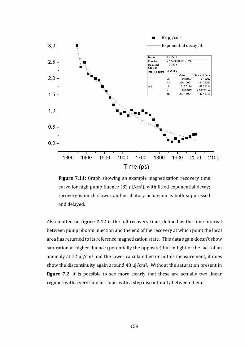
159
Figure 7.11: Graph showing an example magnetization recovery time
curve for high pump fluence (82 µJ/cm2), with fitted exponential decay;
recovery is much slower and oscillatory behaviour is both suppressed
and delayed.
Also plotted on figure 7.12 is the full recovery time, defined as the time interval
between pump photon injection and the end of the recovery at which point the local
area has returned to its reference magnetization state. This data again doesn’t show
saturation at higher fluence (potentially the opposite) but in light of the lack of an
anomaly at 72 µJ/cm2 and the lower calculated error in this measurement, it does
show the discontinuity again around 48 µJ/cm2. Without the saturation present in
figure 7.2, it is possible to see more clearly that these are actually two linear
regimes with a very similar slope, with a step discontinuity between them.
82 µJ/cm2
Exponential decay fit
160
Figure 7.13: Graph showing time constant τ as a function of pump
fluence (black), showing the recovery time from each maximum
demagnetization state; and total recovery time (blue), which includes the
time from the initial pump event, showing the total time associated with
elevated energy in the spin reservoir.
This recovery represents the time taken for the effective field vector Heff to return
to its equilibrium minimum energy state. This timescale is dominated by the change
in the magnetic anisotropy energy, Eani and the demagnetization energy, Edem as
well as a transfer of angular momentum. The relaxation takes place by the transfer
of energy and angular momentum to the environment and to the lattice reservoir.
Relaxation to the environment will occur primarily to the surrounding GdFe rather
than to the substrate, due to stronger coupling. As the surface area of the laser
stimulated region is much smaller than the volume this will be a limited, but
constant, energy sink. Relaxation from spin to the lattice is dependent on the spin-
orbital coupling between them. This can be analyzed by comparison between the
dissipation curves for lattice and spin reservoirs shown from the total Kerr signal
recovery time (displayed in figure 7.13) and the reflectivity recovery time
Ker
r si
gnal
rec
ove
ry t
ime,
τ (
ps)
Pump fluence (µJ/cm2)
To
tal e
lev
ated
en
ergy
tim
e (p
s)

161
(displayed in figure 7.3). The relationship between the two recovery mechanisms
becomes more obvious when replotted against each other in figure 7.13.
Figure 7.13: Comparison of energy dissipation from spin reservoir
(black), (Kerr signal) and lattice reservoir (red, dominant temperature
reservoir over long timescale represented in Reflectivity signal).
For low fluence, the magnetization recovery is significantly faster than the
reflectivity recovery, by ~8x (400 ps). It can be inferred from this data that angular
momentum loss from the lattice to the environment is limited at ~400 ps, and its
capacity to dissipate at this rate is not at all challenged; angular momentum transfer
from the spin to lattice is fast enough that it can be dissipated too. At ~42 µJ/cm2 an
equivalent time scale is reached, and the relaxation of spin plateaus. As this has
already been identified as the magnetization compensation temperature, this
behaviour can be attributed to the stimulated region losing net moment and its
recovery being dominated by the spin-lattice relaxation. Above TMcomp the dominant
moment has reversed, and the spin-orbital coupling to the Fe is now most important.
Pump fluence (µJ/cm2)
To
tal e
lev
ated
en
ergy
tim
e (p
s)

162
As this is lower in Fe, [5] it follows that the spin-lattice relaxation is weaker,
reducing the rate of dissipation of the spin reservoir but also of the lattice reservoir,
which is now ‘drip-fed’ energy and angular momentum. This is shown in figure
7.14. After a certain time, the lattice reservoir reaches equilibrium with the
environment, and the spin reservoir consistently takes ~200 ps longer to finally
dissipate. This will be due to a combination of fast dissipation of a lower energy
density from the lattice (once the energy from the initial electron-lattice relaxation
has dissipated) and an increased importance of the spin-environment loss channel.
Figure 7.15: Schematic showing energy and angular momentum gain
and loss channels. Spin lattice relaxation is dependent on the dominant
moment’s spin-orbit coupling, which is Gd at low temperatures, and
swaps to Fe above TMcomp.
Magnetic Precessional Frequency
In order to analyse the precessional information more accurately, it was necessary
to extract it from the underlying recovery curve. Where that recovery represents
the vector orientation of the effective field, Heff, relative to its initial state, the
procession details the motion of the net magnetization vector, M. To isolate this

163
information, the recovery curve, obtained above (from the red circles in figures 7.8
and 7.9), was subtracted from each plot; this is referred to as the residual. An
example of this result is shown in figures 7.15 and 7.16. Each residual was analysed
following two contrasted methods, and compared. Also shown is the first method:
a damped sinusoidal curve fit plotted against the residual data following equation
2.16 (more details in chapter 2). Of particular interest are the damping factor, τd
and f, the frequency of oscillation, which are related to the damping constant in the
Landau-Lifshitz Gilbert (LLG) equation (written again here in equation 2.18). For
low temperatures, this equation represents the combined coherent precession of
the net moment of both sublattices, which remain fixed relative to each other by
their exchange coupling. For higher temperatures, this approximation becomes less
physical as the sublattices decouple and begin to precess around their own separate
effective field vectors.
Mp(t) = M0 + Aexp(−t/τd) × sin(2πf(t − φ0)) (2.19)
dM/dt = −γ[M × Heff] + αMS−1[M × dM/dt] (2.18)
It can be seen here that each residual showed an oscillatory waveform, which took
at least half an oscillation to reach a maximum before behaving similarly to a
damped sinusoid even at the highest fluence, despite being particularly obscure in
the raw data. As can also be seen, the superimposed sinusoidal fits are not
adequately representative to draw conclusions for the damping parameter, but are
able to provide a set of values for frequency, plotted below in figure 7.19 and
discussed further later.

164
Figure 7.15: Example of magnetic precession residual, after removing
recovery slope low fluence measurement (black) (25 µJ/cm2), with fitted
sinusoidal decay (red).
Figure 7.16: Example of magnetic precession residual, after removing
recovery slope low fluence measurement (black) (82 µJ/cm2), with fitted
sinusoidal decay (red).
25 µJ/cm2
Sinusoidal decay fit
82 µJ/cm2
Sinusoidal decay fit

165
Additionally this technique was undertaken from the second definition of recovery
time, previously discussed and highlighted in figures 7.8 and 7.9 as blue circles.
This gave further confirmation of the significance of the temperature point
associated with ~4 (arb. units) reflectivity, by showing a sharp transition in
oscillation frequency at this time/temperature. An example is shown in figure 7.17
below for 65 µJ/cm2.
Figure 7.17: Residual for 65 µJ/cm2 fluence plot. This shows the two
frequencies, separated by a temperature boundary.
This recovery time also correlated well with a second reflectivity value of ~6.25.
This second set of residuals was used to then calculate fast Fourier transforms
(FFTs) to analyse these oscillations further in the frequency domain. A peak finding
function then provided the resonance frequencies with amplitudes, along with their
full width half maxima (FWHM) which provided the associated error. For the series,
a pair of frequencies was observed, shown in figure 7.18. These are plotted
alongside the equivalent frequency, f, obtained from the curve fitting method in
figure 7.19.
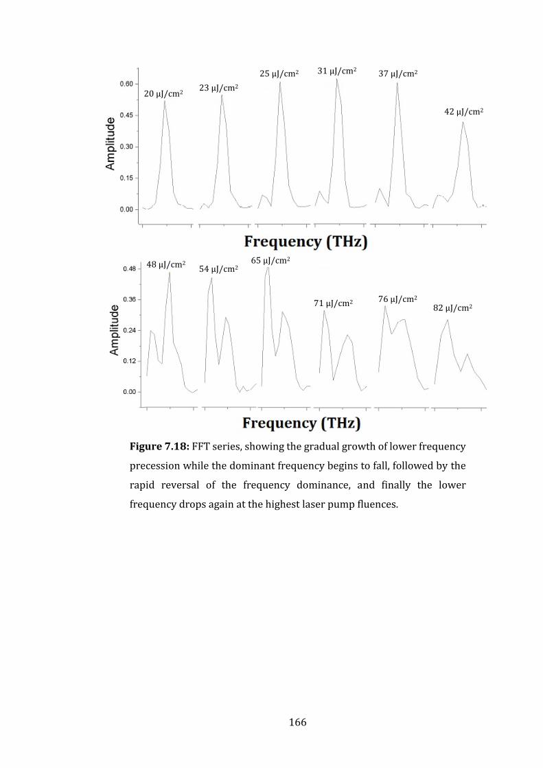
166
Figure 7.18: FFT series, showing the gradual growth of lower frequency
precession while the dominant frequency begins to fall, followed by the
rapid reversal of the frequency dominance, and finally the lower
frequency drops again at the highest laser pump fluences.
42 µJ/cm2
37 µJ/cm2 31 µJ/cm2 25 µJ/cm2
23 µJ/cm2 20 µJ/cm2
82 µJ/cm2 76 µJ/cm2 71 µJ/cm2
65 µJ/cm2 54 µJ/cm2 48 µJ/cm2

167
Figure 7.19: Comparison of FFT frequency vs curve fitted frequency for
coherent precession regime. Shows slow increase with fluence followed
by a significant drop off after 71 µJ/cm2, lower frequency oscillation
observed at higher temperature becomes stronger at higher fluences.
Figure 7.20: Graph showing resonance amplitudes from FFT as a
function of pump fluence for both oscillation frequencies observed. This
shows swapping of dominant precessional mode after TMcomp which is
also then quenched at TAcomp.
Pump fluence (µJ/cm2)
Pump fluence (µJ/cm2)

168
These frequencies are separated by a temperature boundary as defined by the
reflectivity of ~4. The higher frequency (referred to here as f1) exists below this
temperature boundary, while the higher frequency, f2, occurs only above it. Figure
7.19 shows f1 calculated by two separate methods and f2 from the FFT alone. Figure
7.20 shows the resonance amplitudes of f1 and f2. Both FFT and sine curve fitted
data of f1 suggest a general upward trend of increasing frequency as a function of
pump fluence, until after 72 µJ/cm2 when a significant reduction is observed. The
change in frequency and amplitude can be related to the torque applied to the local
macrospin, discussed in chapter 2 and reprinted here in equation 2.9.
dM(t)/dt = −γ [M(t) × Heff] (2.9)
In order to interpret this data, it is important to consider the relative dynamic
behaviour of the two sublattices within the different regimes, which can be divided
into three based on the temperatures reached: low fluence (20-31 µJ/cm2),
intermediate fluence (31-54 µJ/cm2) and high fluence (65-82 µJ/cm2).
● At low temperature, the the Gd and Fe sublattices are exchange coupled and
coherent precession with little reduction in M(t) is observed. As this region
is below the magnetization compensation temperature TMcomp, the Gd
sublattice moment dominates the magnetism. This results in lower
frequency, higher amplitude oscillations for f1, while f2 is very weak.
● Once the fluence is high enough to increase the local lattice temperature
above TMcomp, the Fe sublattice dominates, and the net moment flips, altering
the frequency. Explanations for why this goes up, rather than down (due to
larger moment) have been discussed by Stanciu et al. [6] but with no
conclusive explanation. This may be due to distortion of the frequency in the
vicinity of the two compensation temperatures. As the temperature
increases in this region, the exchange coupling between the sublattices
begins to weaken and f2 begins to become more prominent.

169
● At very high fluence, the exchange coupling reaches a minimum as the
amplitude of f2 maximizes. Here there is a divergence of frequency f1 which
corresponds to the angular momentum compensation temperature TMcomp.
The exchange mode is similarly quenched at this fluence, but grows again at
higher temperatures, as the frequency f1 begins to rapidly drop away,
corresponding to the loss of the FMR mode.
Magnetic Precession Damping
The final property of use which can be obtained from this series, is the damping of
the spin precession, which allows a direct calculation of the Gilbert damping
parameter used in the LLG equation to describe spin orbit relaxation.
Figure 7.21: Graphs showing examples of cropped FMR mode
precession data with damped sinusoidal fitting.
In order to more accurately calculate the precession damping, the residual data
collected into figures 7.4 and 7.16 was selectively refitted, specifying a new starting
time to coincide with the start of the largest oscillation. This initial growth in the
42 µJ/cm2 20 µJ/cm2
82 µJ/cm2 76 µJ/cm2
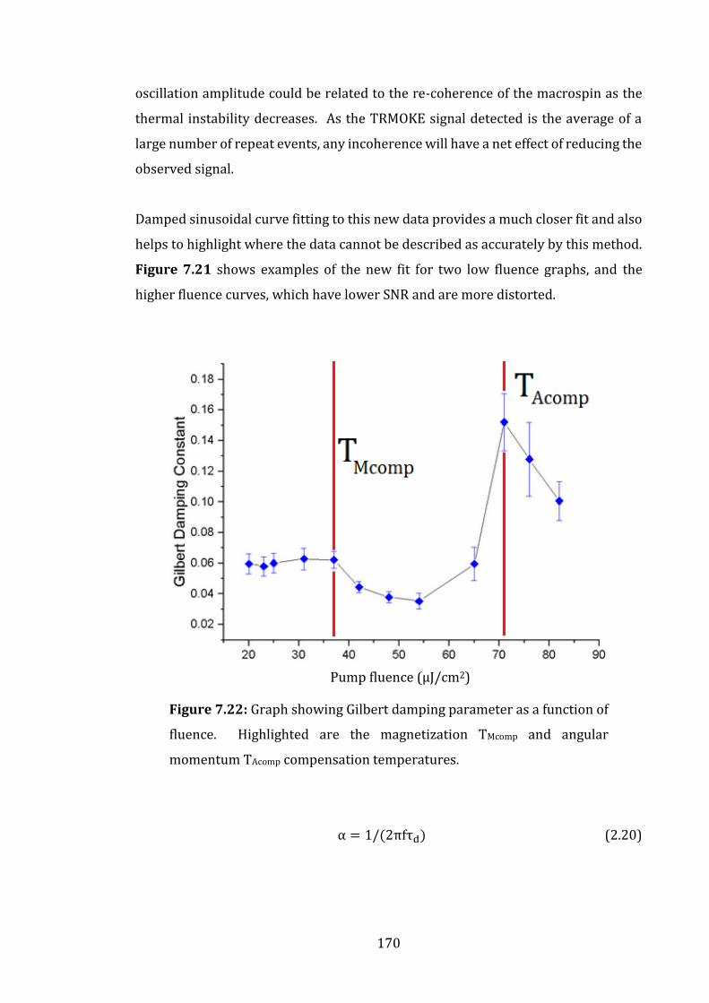
170
oscillation amplitude could be related to the re-coherence of the macrospin as the
thermal instability decreases. As the TRMOKE signal detected is the average of a
large number of repeat events, any incoherence will have a net effect of reducing the
observed signal.
Damped sinusoidal curve fitting to this new data provides a much closer fit and also
helps to highlight where the data cannot be described as accurately by this method.
Figure 7.21 shows examples of the new fit for two low fluence graphs, and the
higher fluence curves, which have lower SNR and are more distorted.
Figure 7.22: Graph showing Gilbert damping parameter as a function of
fluence. Highlighted are the magnetization TMcomp and angular
momentum TAcomp compensation temperatures.
α = 1/(2πfτd) (2.20)
Pump fluence (µJ/cm2)

171
From the FMR mode frequency f1 and exponential sine damping coefficient, τd, the
Gilbert damping parameter, α, was calculated with equation 2.21, detailed in
chapter 2. This data provides a systematic method of measurement and is shown
in figure 7.22 above. This plot confirms the analysis of the precession frequencies
in the previous section, showing both the angular momentum, TAcomp, and
magnetization, TMcomp, compensation temperatures clearly.
7.3 Summary
A series of increasing pump fluence magneto-optic measurements has been
analyzed to extract the characterizing features of a chosen composition ratio of the
rare earth-transition metal alloy GdFe. These features provide an important insight
into both the energy and angular momentum transfer interactions occurring on a
picosecond timescale between the electron, lattice and spin thermodynamic
reservoirs associated with an irradiated region of the sample. Several nonlinearity
features have been observed, which together build up a detailed timeline of the
dynamics. At each step these have been related back to the local lattice temperature,
proportional to the reflectivity response.
7.3.1 Evidence for Magnetization Compensation Temperature
During the demagnetization process a critical reflectivity of ~4V has been identified,
which has been attributed to the spin reservoir transitioning up through the
magnetization compensation temperature TMcomp by three observations:
● Above this temperature, a short lived magnetization recovery is observed.
This corresponds to the transient ferromagnetic state reported theoretically
by other groups [7] [8] and recently observed experimentally in X-ray
Magnetic Circular Dichroism (XMCD) data [9], but not reported in
experimental time resolved MOKE.
● The time taken for the 4f Gd and 3d Fe spin orbital thermal reservoirs to
equilibrate increased by as much as 175% at this temperature.

172
● At this temperature a step change in the peak reflectivity is observed,
indicating a sudden increase in peak temperature experienced by the sample
area.
During the recovery, more evidence that the reflectivity of ~4V corresponds to
TMcomp is provided by the following observations:
● A significant transition between non- and highly fluence dependent regimes
is observed in the lattice relaxation time for fluences which raise the
temperature above this point. This is due to a change from Gd dominated to
Fe dominated spin-orbital coupling to the lattice. The smaller coupling
offered by Fe results in a slower ‘drip fed’ transfer of energy and angular
momentum which causes the slowing of its recovery.
● A sharp transition in precessional modes is observed at this threshold. A
lower frequency exchange mode is observed above the threshold, and a
higher frequency FMR mode coherent precession is consistently observed
below. The exchange mode is caused by higher temperatures weakening the
exchange coupling between the sublattices and causing them to precess
around divergent effective field vectors. It is seen to grow in strength from
this temperature.
● The coherent precession FMR mode is seen to decrease in strength
dramatically from this point and show a limited increase in frequency in
agreement with observations reported by Stanciu et al. [6]
● The Gilbert damping, calculated from the FMR mode decay and frequency,
showed a decline again at this transition, indicating that the spin-orbit
coupling was reduced, corroborating the interpretation of the lattice
relaxation time mechanism.
173
7.3.2 Evidence for Angular Momentum Compensation
Temperature
During the ultrafast demagnetization process, a higher temperature critical point
was also observed corresponding to a reflectivity value of ~6.25V, which was again
consistent across each fluence measurement. This was interpreted as the angular
momentum compensation temperature TAcomp and manifested in the following
ways:
● The observed phenomenon attributed to the ferromagnetic transient state
sharply increased in amplitude above this temperature.
● The time taken for the irradiated area to fully demagnetize peaked at this
temperature after which it begins to decrease again. This enhancement of
the demagnetization rate is indicative of meeting an energy threshold.
Additionally, the recovery at higher fluences showed three key features
corresponding to a turning point at TAcomp:
● The frequency of the FMR mode increased underwent a small but significant
increase followed by a decline, consistent with theory. From reports [6] it is
expected that the frequency diverges around this point and higher fluence
resolution might uncover this.
● The exchange mode is observed to quench just below this fluence, before
increasing again. As the exchange mode softens, it begins to synchronise with
the FMR mode around TAcomp again consistently with literature.
● The Gilbert damping shows the strongest corresponding response, in line
with previous reports, confirming that this is in fact TAcomp.
The observation of a strong increase in damping along with a rise in FMR frequency
at TAcomp conveys the importance of this material for spintronic application. These
174
characteristics lead to the ability to perform ultrafast reversal of magnetization
direction for magneto-optic recording media.
7.4 References
[1] F. Radu, et al., Nature. Comms. 1728, 1 (2012)
[2] Andrei Kirilyuk, et al. Reviews of Modern Physics, 82 (2010)
[3] J. Åkerman, Science 308, 508 (2005)
[4] C. Felser, G. h. Fecher, Spintronics: From Materials to Devices (Springer Verlag,
Berlin, 2013)
[5] J. Stöhr, H. C. Siegmann, Magnetism, (Solid-State Sciences Springer Verlag,
Berlin, 2006)
[6] C. D. Stanciu, et al., Phys. Rev. B, 73, 220402(R) (2006)
[7] S. Weinholdt, et al., Phys. Rev. B, 88, 020406(R) (2013)
[8] U. Atxitia, et al., Phys. Rev. B, 87, 224417 (2013)
[9] I. Radu, et al., Nature (London) 472, 205 (2011)

175
Chapter 8
Conclusions & Further Work
Both of the materials studied in this project, half-metallic Fe3O4 (magnetite) and the
rare-earth transition metal alloy GdFe represent important aspects of spintronic
research [1] [2]. Each material contains its own set of unique challenges and
opportunities.
8.1 Discussion of Post-Oxidized Fe3O4
8.1.1 Discussion of Results
In this work, the nature of post-oxidized Fe films has been explored with a particular
interest in the depth and quality of the oxidation process and the phase of iron oxide
produced. It is noteworthy that the growth mechanism appears to produce the
Fe3O4 inverse spinel structure with ease and that the formation of APB defects is
functionally identical to that of a more standard island growth process.
This investigation would imply that single crystal Fe3O4 can be produced by this
method and in fact benefits from a short oxidation time. Further oxidation rather
than extending the depth of the film results in replacing the B site Fe ions, explaining
the poor magnetic performance by inhibiting the ferromagnetic exchange and

176
superexchange interactions between the Fe2+ and Fe3+. This is confirmed by the
relatively low disorder observed in (001) cross-section HRTEM, compared to much
higher disorder observed in (011) cross-section HRTEM, which resolves the B site
ions separate from the oxygen super-lattice.
The observation of periodic defects between the oxidized and unoxidized layers
appear as expected for the lattice mismatches of Fe3O4 (001)||Fe (011) and for
Fe(011)||MgO(001). This shows again how robust this growth process is, with both
layers epitaxially related to their under layer, with only 1-2 atomic planes of
transition observed. This type of limited depth oxidation has been observed
elsewhere [3], however the sharpness of the interface in this case is particularly
noteworthy.
This presents a useful method of producing a multilayer material with an Fe||Fe3O4
interface, with potential applications in spin injection device tests. The thick Fe
layer, exchange-coupled to the thin Fe3O4 layer would lower its coercivity and
increase its remanence. A current passed through this structure would experience
an enhanced spin polarization by the Fe3O4 before potentially being injected into a
semiconductor.
8.1.2 Further Research
Further research in this field must consider shorter post-oxidation times and
observe the lower limit of the oxide formation process. A sweet spot can be
identified by the crystallographic and magnetometric techniques detailed in this
thesis and Fe||Fe3O4 or pure Fe3O4 devices can be grown to begin testing of spin
injection efficiencies. This was an intended avenue of investigation during this
project, but was postponed due to uncontrollable logistics issues with the growth
stage.

177
8.2 Fluence Dependent Magneto-Dynamics in GdFe
8.2.1 Discussion of Results
This investigation has uncovered four key features in the temperature dependent
behaviour of a key spintronic material GdFe. 1. A discontinuity in the ultrafast peak
reflectivity with fluence. 2. An observed transient picosecond timescale magnetic
moment recovery. 3. A relationship between the lattice and spin relaxation rates. 4.
A low frequency exchange mode softening between the compensation
temperatures. These manifest from the unique interaction between the
antiferromagnetically coupled sublattices. These provide further insight into the
energy and angular momentum exchange taking place, as well as a robust
methodology for characterizing such materials in future.
At fluences which raise the peak temperature above TMcomp, a step in the peak
reflectivity was observed. In other words, for a proportionally larger energy
density, a constant extra level of heat is produced above this point. This would imply
that either the specific heat capacity of the lattice has reduced by a fixed value, or
that the electron->lattice and electron->spin energy transfer ratios have been
altered. The first option is unlikely, but the second is plausible as a result of the
swapping of the dominant sublattices. This could also be a result of, and evidence
for, the fast coherent phonon spin-lattice exchange, which is allowed by the large 4f
spin-orbital coupling, but inhibited by the much smaller 3d value.
The observed picosecond magnetic moment recovery is produced by the transient
ferromagnetic state. This is consistent with the spin temperature rapidly
transitioning through the magnetization compensation point and reversing the
dominance of the field. This has been reported experimentally in XMCD data [4] ,
but not with the clarity observed in this system. It shows a strong agreement with
the interpretation of the other features in this dynamic investigation.
The relaxation of the spin and lattice systems have been observed to be strongly
interdependent, as a function of fluence. This provides a clear indication of the
timescales of energy and angular momentum transfer. As the lattice-environment
178
is stronger than the spin-environment coupling, exchange will predominantly be by
transfer out of the spin system and into the lattice. At low fluence the coupling is
strong between them, due to the dominance of the Gd sublattice, and energy transfer
is limited only by lattice coupling to the environment (at around 400 ps). As the
fluence rises, the Fe sublattice takes over dominance and the spin-orbit coupling
significantly weakens. This slows the spin-lattice exchange, creating a longer lived
elevated energy state in the lattice. Lattice relaxation shows a consistent 200 ps lag
behind spin relaxation in this regime. This would imply that spin-environment
exchange plays a larger role, which would be consistent with the itinerant nature of
the now dominant 3d Fe. A single point in this region shows a 100 ps lag between
the lattice and spin relaxation, corresponding to the angular momentum
compensation state. These interpretations are based on a variable strength of the
spin-orbital coupling, which is consistent with and supported by the independently
measured Gilbert damping results.
The observation of a low frequency oscillation is interpreted as the manifestation of
the exchange mode. This interpretation can be supported by comparison to that
made by Mekonnen et al. [5] to assess the validity of this conclusion. In their paper
Femtosecond Laser Excitation of Spin Resonances in Amorphous Ferrimagnetic Gd1-
xCox Alloys the authors quote an exchange mode of the order of ~70 GHz, while this
investigation finds a much lower frequency exchange mode ~1.5 GHz. The
frequency of the exchange mode is found via the gyromagnetic ratios of each
sublattice (γRE, γTM)and the interatomic exchange coefficient between them
λRE−TM. This is presented by Mekonnen in the form of equation 3.3, where x is the
relative concentration of the transition metal, TM and 1 − xis that of the rare earth
RE.
fex = λRE−TMγREγTM[xMTM/γTM − (1 − x)MRE/γRE] (3.3)
While this will not be affected by external field strength like the FMR mode, it can be
expected that this system will have a weaker exchange mode by comparing Fe to Co.
The gyromagnetic ratios (γ/2π) of Fe [6] and Co [7] are 0.1382 kHz/G and 1.0054
kHz/G respectively, making this an order of magnitude smaller in Fe. So for a GdFe
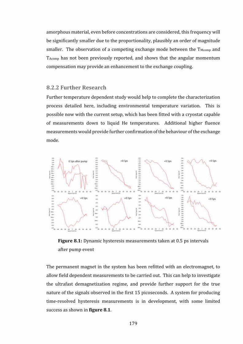
179
amorphous material, even before concentrations are considered, this frequency will
be significantly smaller due to the proportionality, plausibly an order of magnitude
smaller. The observation of a competing exchange mode between the TMcomp and
TAcomp has not been previously reported, and shows that the angular momentum
compensation may provide an enhancement to the exchange coupling.
8.2.2 Further Research
Further temperature dependent study would help to complete the characterization
process detailed here, including environmental temperature variation. This is
possible now with the current setup, which has been fitted with a cryostat capable
of measurements down to liquid He temperatures. Additional higher fluence
measurements would provide further confirmation of the behaviour of the exchange
mode.
Figure 8.1: Dynamic hysteresis measurements taken at 0.5 ps intervals
after pump event
The permanent magnet in the system has been refitted with an electromagnet, to
allow field dependent measurements to be carried out. This can help to investigate
the ultrafast demagnetization regime, and provide further support for the true
nature of the signals observed in the first 15 picoseconds. A system for producing
time-resolved hysteresis measurements is in development, with some limited
success as shown in figure 8.1.
180
8.3 Concluding Remarks
This thesis has explored and demonstrated a number of experimental techniques
capable of characterizing the critical parameters involved in optimizing a material
for application in a spintronic device. This has involved preparation and
observation of microscopy images as well as the construction and use of a
femtosecond pump-probe MOKE apparatus. A number of new and supported
observations have been made, which can be used to feedback to growth of improved
materials.
8.4 References
[1] S. A. Wolf, et al., Magn. and Mat., 294, 1488 (2001)
[2] A. Hirohata and K. Takanashi, J. Phys. D: Appl. Phys., 47, 193001 (2014)
[3] N. Cabrera and N. F. Mott, Rep. Prog. Phys. 12, 163 (1949)
[4] I. Radu, et al., Nature (London) 472, 205 (2011)
[5] A. Mekonnen, et al., Phys. Rev. Lett., 107, 117202 (2011)
[6] G. G. Scott, Phys. Rev., 99, 1241 (1955)
[7] R. E Walstedt, et al., Phys. Rev., 162, 301 (1967)
181
Glossary
Å Angstrom
AOM Acousto-Optic Modulator
APB Anti-Phase Domain Boundary
Ar Argon
BBO Barium Borate
Fe Iron
Fe3O4 Magnetite
FFT Fast Fourier Transform
FMR Ferromagnetic Resonance
FWHM Full-Width Half Maximum
Gd Gadolinium
GMR Giant Magneto Resistance
GVD Group Velocity Dispersion
ħ Planck Constant
Hc Magnetic Coercivity
HDD Hard Disk Drive
Heff Effective Magnetic Field Vector
(HR)TEM (High-Resolution) Transmission Electron Microscopy
JEOL Japan Electron Optics Laboratory Company
Jex Exchange Integral
LBO Lithium Triborate
LLG Landau-Lifshitz Gilbert equation
MBE Molecular Beam Epitaxy
MOKE Magneto Optic Kerr Effect
MR Magnetic Rememance
MRAM Magnetic Random Access Memory
MS Saturation Magnetisation
Nd Neodymium
O Oxygen
Oe Oersted

182
PSD Phase Sensitive Detection
RE Rare Earth Metal
SADIFF Select-Area Diffraction
SHG Second Harmonic Generating
Si Silicon
SNR Signal to Noise Ratio
TC Time Constant
Ti Titanium
TM Transition Metal
μB Bohr Magneton
VSM Vibrating Sample Magnetometry
XMCD X-ray Magnetic Circular Dichroism
YVO Yttrium Vanadate
Antiferromagnet A magnetic material whose sublattice moments sit
opposite to each other and exactly cancel.
Birefringence The property of a material causing it to have a
refractive index dependent on the polarization and
direction of light.
Curie temperature A phase transition temperature above which magnetic
materials undergo a sudden reversible loss of
magnetic order.
Exchange A quantum mechanical effect which occurs only
between identical particles and leads to moment
alignment required for ferromagnetism.
Fermion A subatomic particle with half-integer spin.

183
Ferrimagnet A magnetic material which exhibits non-perfectly
cancelling antiferromagnetism, such that some net
moment exists.
Ferromagnet A material susceptible to magnetization.
Fluence Radiant energy received by a surface per unit area.
Kerr Effect A change in the refractive index of a material in
response to an applied field.
Magnetic Moment A property of magnetic materials which interacts with
an applied field to produce a mechanical moment.
Magnetoresistance The extent to which a material’s electrical resistance is
modified by an externally applied magnetic field.
Precession The movement of an axis of rotation around a second
axis due to a torque force acting to move the first axis.
Spin A quantum mechanical intrinsic angular momentum
exhibited by a subatomic particles and atomic nuclei.
Spintronic Spin Transport Electronics (portmanteau).
Ultrafast Timescales on the order of less than 100 picoseconds.
Voigt Effect A magneto-optical phenomenon which causes
polarized light to rotate and elliptize within an
optically active medium.


