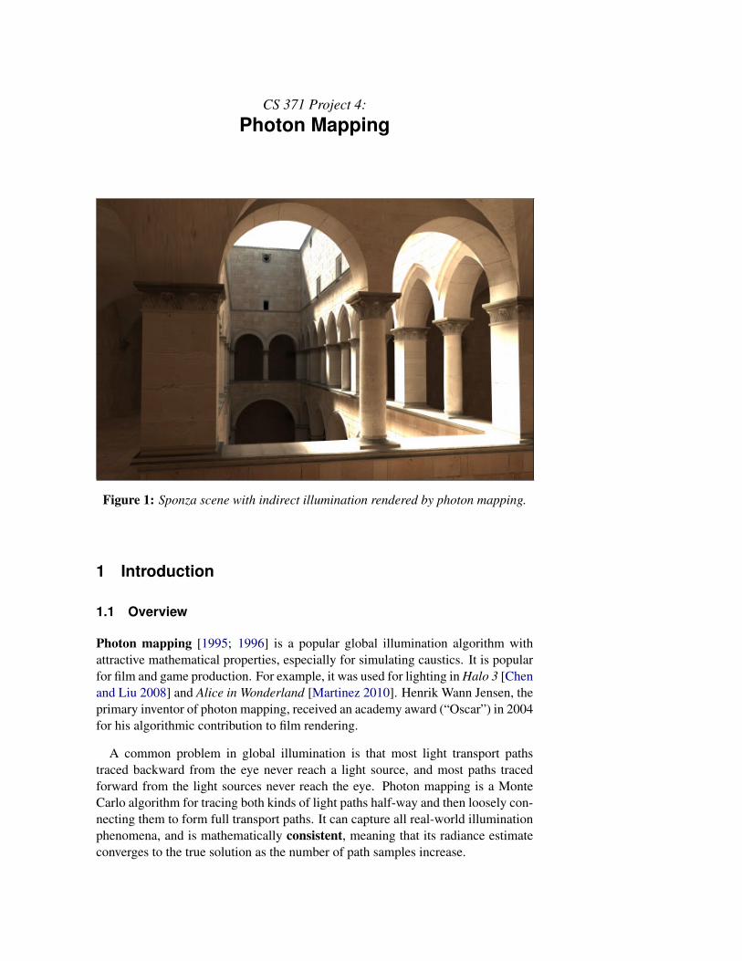
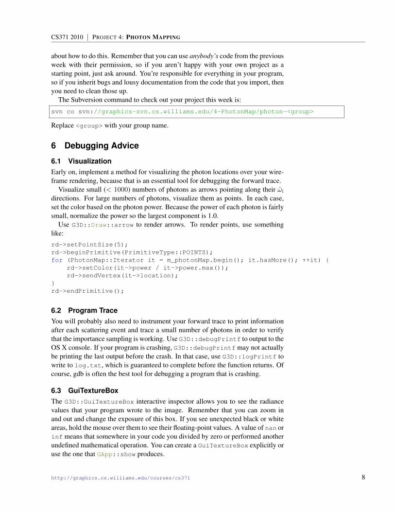
CS 371 Project 4: Photon Mapping Figure 1: Sponza scene with indirect illumination rendered by photon mapping. 1 Introduction 1.1 Overview Photon mapping [1995; 1996] is a popular global illumination algorithm with attractive mathematical properties, especially for simulating caustics. It is popular for film and game production. For example, it was used for lighting in Halo 3 [Chen and Liu 2008] and Alice in Wonderland [Martinez 2010]. Henrik Wann Jensen, the primary inventor of photon mapping, received an academy award (“Oscar”) in 2004 for his algorithmic contribution to film rendering. A common problem in global illumination is that most light transport paths traced backward from the eye never reach a light source, and most paths traced forward from the light sources never reach the eye. Photon mapping is a Monte Carlo algorithm for tracing both kinds of light paths half-way and then loosely con- necting them to form full transport paths. It can capture all real-world illumination phenomena, and is mathematically consistent, meaning that its radiance estimate converges to the true solution as the number of path samples increase.
Transcript
CS 371 Project 4:
Photon Mapping
Figure 1: Sponza scene with indirect illumination rendered by photon mapping.
1 Introduction
1.1 Overview
Photon mapping [1995; 1996] is a popular global illumination algorithm withattractive mathematical properties, especially for simulating caustics. It is popularfor film and game production. For example, it was used for lighting in Halo 3 [Chenand Liu 2008] and Alice in Wonderland [Martinez 2010]. Henrik Wann Jensen, theprimary inventor of photon mapping, received an academy award (“Oscar”) in 2004for his algorithmic contribution to film rendering.
A common problem in global illumination is that most light transport pathstraced backward from the eye never reach a light source, and most paths tracedforward from the light sources never reach the eye. Photon mapping is a MonteCarlo algorithm for tracing both kinds of light paths half-way and then loosely con-necting them to form full transport paths. It can capture all real-world illuminationphenomena, and is mathematically consistent, meaning that its radiance estimateconverges to the true solution as the number of path samples increase.
CS371 2010 | PROJECT 4: PHOTON MAPPING
1.2 Educational GoalsIn this project you will implement a photon mapping framework that can render aphotorealistic image of any scene for which you can provide a suitable BRDF andgeometric model. You will work from resources in the computer science literatureincluding Jensen’s paper [1996] and his SIGGRAPH course notes. Along the wayyou will:
• Learn to read a computer science paper and implement an algorithm from it.
• Design your own structure for a complex mathematical program.
• Learn to create and perform experimental analysis without explicit guidance.
• Solve the kind of radiometry problems we’ve seen in lecture on your own.
• Gain experience with Monte Carlo importance sampling, an essential tech-nique for graphics and other high-performance computing domains includingcomputational biology, finance, and nuclear science.
• Gain experience with the hash grid spatial data structure for expected O(1)insert, remove, and linear-time gather in the size of the query radius andoutput.
• Use the trait and iterator software design patterns employed for statically-typed polymorphic data structures in C++.
1.3 ScheduleThis is a challenging, pair-programming project that builds extends the previousray tracer project. The program will only add about 100 lines to your existingray tracer. However, they are mathematically sophisticated lines and you will takeresponsibility for the program design and experiment design yourself this weekinstead of having them given to you in the handout.
Note that you have three extra days and one extra lab session compared to mostprojects because the project spans Fall reading period. If you plan to take a four-day weekend I recommend completely implementing and debugging the forwardtrace before you leave.
As a reference, my implementation contained 9 files, 420 statements, and 300comment lines as reported by iCompile. I spent substantially longer debugging thisprogram than I did for the other projects this semester.
Out: Tuesday, October 5Checkpoint 1 (Sec. 3.2): Thursday, October 7, 1:00 pmCheckpoint 2 (Sec. 3.3): Thursday, October 14, 1:00 pm
Due: Friday, October 15, 11:00 pm
2 Rules/Honor Code
You are encouraged to talk to other students and share strategies and programmingtechniques. You should not look at any other group’s code for this project or use
code from other external sources except for: Jensen’s publications, the pbrt library,RTR3 and FCG textbooks, materials presented in lecture, and the G3D library (aslimited below). You may look at and use anyone’s code from last week’s project,with their permission.
During this project, you may use any part of the G3D library and look at all of itssource code, including sample programs, with the exception of SuperBSDF::scatter,which you may not invoke or read the source for.
You may share data files and can collaborate with other groups to create test andvisually impressive scenes. If you share a visually impressive scene with anothergroup, ensure that you use different camera angles or make other modifications todistinguish your image of it. On this project you may use any development stylethat you choose. You are not required to use pure side-by-side pair programming,although you may still find that an effective and enjoyable way of working.
3 Specification
1. Implement the specific variant of the photon mapping [Jensen 1996] algo-rithm described in Section 3.1.
2. Create a graphical user interface backed by functionality for:
(a) Selecting resolution
(b) Real-time preview with camera control
(c) Rendering the view currently observed in the real-time preview
(d) Setting RenderSettings::numEmittedPhotons
(e) Setting RenderSettings::maxForwardBounces and RenderSettings::maxBackwardBounces
(f) Enabling explicit direct illumination (vs. handling direct illuminationvia the photon map)
(g) Enabling shadow rays when direct illumination is enabled
(h) Enabling real-time visualization of the stored photons over the wire-frame (see Section 6.1).
(i) Setting the photon gather radius r, RenderSettings::photonRadius
(j) Displaying the number of triangles in the scene
(k) Displaying the forward and backward trace times
3. Document the interfaces of your source code using Doxygen formatting.
4. Devise and render one visually impressive scene of your own creation, asdescribed in Section 3.4.
5. Devise and render as many custom scenes as needed to demonstrate correct-ness or explore errors and performance, as described in Section 3.4.
6. Produce the reports described in Sections 3.2-3.4 as a cumulative Doxygenmainpage.
3.1 DetailsPhoton mapping algorithm was introduced by Jensen and Christensen [1995] andrefined by Jensen [1996]. Use those primary sources as your guide to the algo-rithm. Additional information about the algorithm and implementation is availablein Jensen’s book [2001] and course notes [2007]. The notes are almost identical tothe book and are available online. Section 7 of this project document summarizesmathematical aspects covered in class that are ambiguous in the original papers.
Make the following changes relative to the algorithm described in the 1996 paper.These increase the number of photons needed for convergence by a constant factorbut greatly simplify the implementation. The algorithm remains mathematicallyconsistent.
1. Do not implement:
(a) The projection map; it is a useful optimization for irregular scenes butis hard to implement.
(b) The illumination maps described in the 1995 paper. Pure photon mapsare today the preferred implementation [Jensen 1996].
(c) The caustic map—just store a single global photon map and do notdistinguish between path types.
(d) Shadow photons; they are an important optimization for area lightsources but are unnecessary for point emitters.
2. Use G3D::PointHashGrid instead of a kd-tree to implement the photonmap data structure. This gives superior performance [Ma and McCool 2002].
3. Ignore the 1995 implementation of the photon class. Instead use a varianton the 1996 implementation: store position, incident direction, and powerfor each photon. Both papers recommend compressing photons. Use a nat-ural floating point representation instead of a compressed one. Do not storesurface normals in the photons.
4. Use a constant-radius gather sphere (as described on page 7 of the 1996paper). When you have that working, you may optionally implement theellipsoid gathering method or the k-nearest-neighbor method and compareperformance and image quality.
5. Implement the algorithm that Jensen calls“direct visualization of the photonmap”1 rather than final gathering. This means that you should not makemultiple ray casts from a point when estimating indirect illumination, butinstead use the radiance estimate from the photon map directly.
Beware that the description of the trace from the eye sounds more complicatedthan it actually is. You’re just going to extend your existing ray tracer by addingindirect light to the direct illumination at every point.
1Jensen refers to the kind of gathering you’re implementing as “visualizing the photon map.” Thisdocument calls that simply “gathering” and the “radiance estimate” and uses “visualization” to referto debugging tools.
3.2 Checkpoint 1 Report (due Thursday, Oct. 7, 1:00 pm)1. Implement Photon class (it need not have any methods!)
2. Give pseudo-code for the entire photon mapping algorithm in your Doxygen Tip: Parts of the pho-
ton mapping algorithm
will be presented in lec-
ture the Wednesday after
the project starts, however
you can begin now be-
cause the handout and pa-
pers contain all of that in-
formation and more.
mainpage.
(a) Almost all of the information that you need is in this handout, but isdistributed so that you have to think and read instead of copying it. Besure to read everything in here.
(b) Use a hierarchical list, with the four major steps at the top level and thedetails inside. Your full pseudo-code, including some LaTeX for theequations should be around 40 lines long.
(c) I recommend using either nested HTML lists (<ol><li>...</ol>)or simple preformatted HTML (<pre>...</pre>) inside a Doxygen\htmlonly....\endhtmlonly block.
(d) The details you need are in the implementation section (7), Jensen’snotes [2007], and McGuire and Luebke’s appendix [2009].
(e) Use actual (and anticipated actual) names of RayTracer methods andmembers in the code so that they will be linked correctly when you re-ally implement them. With careful use of \copydoc and \copybriefyou can avoid typing the documentation twice.
(f) Give all details for the implementation of RayTracer::emitPhoton(discussed Wednesday in class).
3. Prove (in your Doxygen mainpage) that the emitted photons collectively rep-resent the total emitted power of the lights,∑
P∈photonsP.Φ =
∑E∈lights
L.Φ. (1)
4. Prove that Lo in Equation 5 has radiance units in your Doxygen mainpage.
5. Show a screenshot of the specified user interface in your Doxygen mainpage.
We will set up the photon map data structure together in the scheduled lab us-ing the trait and iterator design patterns, and you will then implement and begindebugging your forward trace.
3.3 Checkpoint 2 Report (due Thursday, Oct. 14, 1:00 pm)Complete a preliminary version of your report and hypothetical results, so that theformatting is done.
Answer the BSDF Diagrams questions from the final report. You can changeyour answer later, but try to get it right the first time.Tip: You should have written the code for the entire program at this point, but it
need not be working correctly yet. This way I can help you work through bugs during
the scheduled lab without having downtime while you generate lots of new code. Your
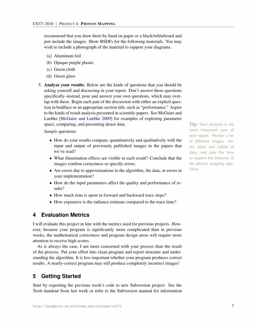
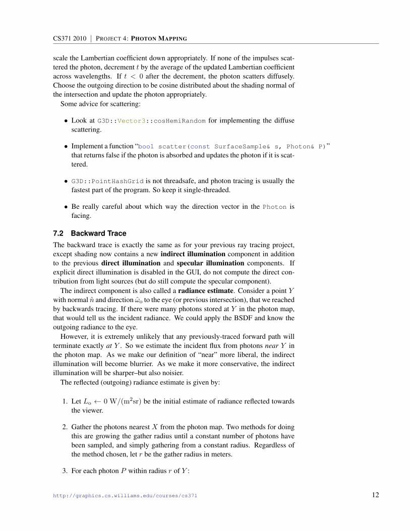
(a) Cardiod caustic from a metalring rendered by Henrik WannJensen using photon mapping.
(b) Cornell box photographicreference image by FrancoisSillion
(c) Sponza atrium ren-dered by Matt Pharr andGreg Humphreys usingphoton mapping.
Figure 2: Classic global illumination test scenes.
forward trace should be working at this point, so you’ll probably spend most of your
time in the scheduled lab debugging the radiance estimate and performing experiments
for your final report.
3.4 Final ReportExtend the mainpage of your Doxygen-generated documentation to include a brief,motivating description of your design (including where each major part of the al-gorithm is implemented), any known bugs and what you know about them, and thefollowing elements. Retain the information from the checkpoint reports.
1. Render the following classic global illumination test scenes, attempting tomatch the reference images as closely as possible: Tip: ifs/ring.ifs
(a) Metal ring from by Jensen [2001] shown in Figure 2(a), http://graphics.ucsd.edu/˜henrik/images/caustics.html
(b) Cornell box photographic reference by Francois Sillion shown in Fig-ure 2(b), http://www.graphics.cornell.edu/online/box/compare.html
(c) Sponza atrium from Pharr’s and Humphreys’s book shown in Figure 2(c),http://www.pbrt.org/scenes_images/sponza-phomap.jpg
2. Show one “teaser” image of a custom scene intended to impress the viewer atthe top of your report. Plan to spend at least three person-hours just creatingthe scene for this image. You may collaborate with other groups on this step.
3. Show other images as needed of custom scenes to demonstrate correctnessin specific cases and to support your discussion.
4. BSDF Diagrams. Create a set of BSDF diagrams as 2D schematics of the3D shape for a fixed angle of incidence, as we commonly draw in lecture.Show the BSDF for red, green, and blue wavelengths (in the appropriatecolors) either side-by-side or overlaid on the same image. To save time, I
recommend that you draw them by hand on paper or a black/whiteboard andjust include the images. Show BSDFs for the following materials. You maywish to include a photograph of the material to support your diagrams.
(a) Aluminum foil(b) Opaque purple plastic(c) Green cloth(d) Green glass
5. Analyze your results. Below are the kinds of questions that you should beasking yourself and discussing in your report. Don’t answer these questionsspecifically–instead, pose and answer your own questions, which may over-lap with these. Begin each part of the discussion with either an explicit ques-tion in boldface or an appropriate section title, such as “performance.” Aspireto the kinds of result analysis presented in scientific papers. See McGuire andLuebke [McGuire and Luebke 2009] for examples of exploring parameterspace, comparing, and presenting dense data. Tip: Your analysis is the
most important part of
your report. Render a lot
of different images, cre-
ate plots and tables of
data, and take the time
to explore the behavior of
the photon mapping algo-
rithm.
Sample questions:
• How do your results compare, quantitatively and qualitatively with theinput and output of previously published images in the papers thatwe’ve read?• What illumination effects are visible in each result? Conclude that the
images confirm correctness or specific errors.• Are errors due to approximations in the algorithm, the data, or errors in
your implementation?• How do the input parameters affect the quality and performance of re-
sults?• How much time is spent in forward and backward trace steps?• How expensive is the radiance estimate compared to the trace time?
4 Evaluation Metrics
I will evaluate this project in line with the metrics used for previous projects. How-ever, because your program is significantly more complicated than in previousweeks, the mathematical correctness and program design areas will require moreattention to receive high scores.
As is always the case, I am more concerned with your process than the resultof the process. Put your effort into clean program and report structure and under-standing the algorithm. It is less important whether your program produces correctresults. A nearly-correct program may still produce completely incorrect images!
5 Getting Started
Start by exporting the previous week’s code to new Subversion project. See theTools handout from last week or refer to the Subversion manual for information
about how to do this. Remember that you can use anybody’s code from the previousweek with their permission, so if you aren’t happy with your own project as astarting point, just ask around. You’re responsible for everything in your program,so if you inherit bugs and lousy documentation from the code that you import, thenyou need to clean those up.
The Subversion command to check out your project this week is:
svn co svn://graphics-svn.cs.williams.edu/4-PhotonMap/photon-<group>
Replace <group> with your group name.
6 Debugging Advice
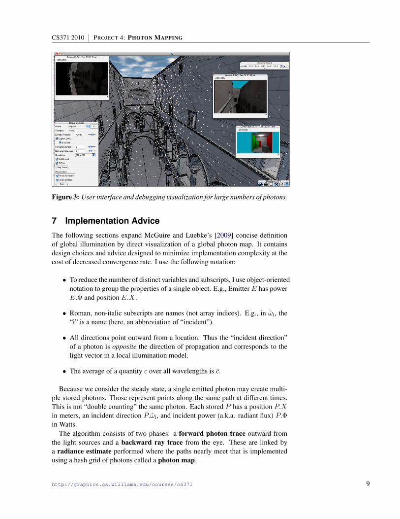
6.1 VisualizationEarly on, implement a method for visualizing the photon locations over your wire-frame rendering, because that is an essential tool for debugging the forward trace.
Visualize small (< 1000) numbers of photons as arrows pointing along their ω̂i
directions. For large numbers of photons, visualize them as points. In each case,set the color based on the photon power. Because the power of each photon is fairlysmall, normalize the power so the largest component is 1.0.
Use G3D::Draw::arrow to render arrows. To render points, use somethinglike:
rd->setPointSize(5);rd->beginPrimitive(PrimitiveType::POINTS);for (PhotonMap::Iterator it = m_photonMap.begin(); it.hasMore(); ++it) {
6.2 Program TraceYou will probably also need to instrument your forward trace to print informationafter each scattering event and trace a small number of photons in order to verifythat the importance sampling is working. Use G3D::debugPrintf to output to theOS X console. If your program is crashing, G3D::debugPrintf may not actuallybe printing the last output before the crash. In that case, use G3D::logPrintf towrite to log.txt, which is guaranteed to complete before the function returns. Ofcourse, gdb is often the best tool for debugging a program that is crashing.
6.3 GuiTextureBoxThe G3D::GuiTextureBox interactive inspector allows you to see the radiancevalues that your program wrote to the image. Remember that you can zoom inand out and change the exposure of this box. If you see unexpected black or whiteareas, hold the mouse over them to see their floating-point values. A value of nan orinf means that somewhere in your code you divided by zero or performed anotherundefined mathematical operation. You can create a GuiTextureBox explicitly oruse the one that GApp::show produces.
Figure 3: User interface and debugging visualization for large numbers of photons.
7 Implementation Advice
The following sections expand McGuire and Luebke’s [2009] concise definitionof global illumination by direct visualization of a global photon map. It containsdesign choices and advice designed to minimize implementation complexity at thecost of decreased convergence rate. I use the following notation:
• To reduce the number of distinct variables and subscripts, I use object-orientednotation to group the properties of a single object. E.g., Emitter E has powerE.Φ and position E.X .
• Roman, non-italic subscripts are names (not array indices). E.g., in ω̂i, the“i” is a name (here, an abbreviation of “incident”).
• All directions point outward from a location. Thus the “incident direction”of a photon is opposite the direction of propagation and corresponds to thelight vector in a local illumination model.
• The average of a quantity c over all wavelengths is c̄.
Because we consider the steady state, a single emitted photon may create multi-ple stored photons. Those represent points along the same path at different times.This is not “double counting” the same photon. Each stored P has a position P.Xin meters, an incident direction P.ω̂i, and incident power (a.k.a. radiant flux) P.Φin Watts.
The algorithm consists of two phases: a forward photon trace outward fromthe light sources and a backward ray trace from the eye. These are linked bya radiance estimate performed where the paths nearly meet that is implementedusing a hash grid of photons called a photon map.
7.1 Forward TraceThe forward photon trace computes the photon map, scattering (“bouncing”) eachphoton a limited number of times. Each emitted photon may produce multiplestored photons. Repeat the following numEmitted times:
1. Select an emitter E ∈ emiters with probability proportionate to its relativepower, averaged over wavelengths:
ρ̄e(E) =E.Φ̄∑
F∈emitters
F.Φ̄. (2)
2. Let E be the selected emitter. Create a new photon P with power2
P.Φ← E.Φ
numEmitted · ρ̄e(E), (3)
and initial position P.X ← E.X at the emitter. For an omnidirectional pointemitter, choose direction P.ω̂i uniformly at random on the sphere. For a spotlight, use rejection sampling against the cone of the spot light to ensure thatthe emitted direction is within the cone.
3. Repeat at most maxForwardBounces times:
(a) Let Y be the first intersection of ray (P.X,−P.ω̂i) with the scene. Ifthere is no such intersection, abort processing of this photon by imme-diately exiting this loop.
(b) Update the photon with P.X ← Y .
(c) Store a copy of photon P in the photon map.
(d) Scatter the photon. If this photon is absorbed instead of scattering, abortprocessing it by immediately exiting this loop (this is Russian roulettesampling of the scattering function). At a surface whose reflectivity isρs that varies with wavelength, let the scattering probability be ρ̄s. Ifthe photon scatters, let its power be updated by P.Φ← P.Φ · ρs/ρ̄s.
If explicit direct illumination is enabled in the GUI, do not store photons on theirfirst bounce, but do still scatter them.
Some advice for the photon forward trace and the photon radiance estimate:
• A spot light has G3D::GLight::spotHalfAngle ≤ π/22Note that the power of an individual photon is small when either numEmitted or |emitters| is
large. Jensen chooses to scale power such that the average photon has power 1.0 at each wavelength,claiming that this avoids underflow and improves floating point accuracy [Jensen 2001]. I believe thisis a misunderstanding of the IEEE floating point format and have not experimentally observed anyloss of precision even when using millions of photons.
• G3D::GLight::color is the power that a spot light would have if it were apoint light. The actual emitted power of the light taking the cone into accountis G3D::GLight::power, which is what you should use. This interfacemakes it so that lights don’t appear to get “darker” at points already withinthe cone when you adjust the cone angle.
• Be really careful with the photon direction convention. It is confusing fortwo reasons. First, the propagation direction is different than the incident di-rection that you eventually want to store. Second, the photon travels betweentwo points during each iteration, and the vectors describing the direction be-tween them point in opposite directions at each end. So your conventionwill be backwards for half of the iteration no matter what you do. Use as-sertions heavily and run targeted experiments with small numbers of photonand small numbers of bounces to ensure that you have this correct. There areseveral places that you will have to negate the photon direction.
• Just as with backwards tracing, you have to bump photons a small amountalong the geometric normal of the last surface hit to avoid getting “stuck”on surfaces. If you see strange diagonal patterns of photons or the photonsgenerally have the same color as the surface that they are on, you aren’tbumping (or are bumping in the wrong direction!)
• Photons store incident illumination–before a bounce.
7.1.1 Scattering
Our BSDF from the previous projects contained a diffuse Lambertian lobe and aglossy Blinn-Phong lobe. The Blinn-Phong lobe could have an infinite exponenton the cosine term, representing a mirror reflection.
Scattering from a finite Blinn-Phong lobe is a little tricky3. Therefore, to sim-plify the implementation you will will approximate the approximate the BSDF dur-ing forward scattering with only a diffuse Lambertian lobe and a mirror-reflectionimpulse.
To implement the scattering, first query the intersection for the impulse(s) andthe Lambertian coefficient. We ignore the glossy coefficient (consider the kinds oferrors this creates, and what it means for the images). Choose a number t uniformlyat random on [0, 1]. The coefficient of an impulse is the probability that a photonscatters along that direction. So, for each impulse, decrement t by the impulse’scoefficient averaged over its wavelengths. If t < 0 after a decrement, the photonscattered in that direction, so update the photon’s information and return it.
The probability of the photon performing Lambertian scattering is the Lamber-tian coefficient scaled by one minus the sum of the impulse coefficients. Thishas nothing to do with the radiometry or the mathematics–it is just the way thatSuperBSDF is defined. It is defined that way so that it is easy to ensure energyconservation. If you increase the impulse probability in the scene file, it is un-derstood that the sampling code (which in this case, you’re the one writing!) will
3Two options are rejection sampling, which can be slow, and an approximate analytic form that iscomplex [Ashikhmin and Shirley 2000].
scale the Lambertian coefficient down appropriately. If none of the impulses scat-tered the photon, decrement t by the average of the updated Lambertian coefficientacross wavelengths. If t < 0 after the decrement, the photon scatters diffusely.Choose the outgoing direction to be cosine distributed about the shading normal ofthe intersection and update the photon appropriately.
Some advice for scattering:
• Look at G3D::Vector3::cosHemiRandom for implementing the diffusescattering.
• Implement a function “bool scatter(const SurfaceSample& s, Photon& P)”that returns false if the photon is absorbed and updates the photon if it is scat-tered.
• G3D::PointHashGrid is not threadsafe, and photon tracing is usually thefastest part of the program. So keep it single-threaded.
• Be really careful about which way the direction vector in the Photon isfacing.
7.2 Backward TraceThe backward trace is exactly the same as for your previous ray tracing project,except shading now contains a new indirect illumination component in additionto the previous direct illumination and specular illumination components. Ifexplicit direct illumination is disabled in the GUI, do not compute the direct con-tribution from light sources (but do still compute the specular component).
The indirect component is also called a radiance estimate. Consider a point Ywith normal n̂ and direction ω̂o to the eye (or previous intersection), that we reachedby backwards tracing. If there were many photons stored at Y in the photon map,that would tell us the incident radiance. We could apply the BSDF and know theoutgoing radiance to the eye.
However, it is extremely unlikely that any previously-traced forward path willterminate exactly at Y . So we estimate the incident flux from photons near Y inthe photon map. As we make our definition of “near” more liberal, the indirectillumination will become blurrier. As we make it more conservative, the indirectillumination will be sharper–but also noisier.
The reflected (outgoing) radiance estimate is given by:
1. Let Lo ← 0 W/(m2sr) be the initial estimate of radiance reflected towardsthe viewer.
2. Gather the photons nearest X from the photon map. Two methods for doingthis are growing the gather radius until a constant number of photons havebeen sampled, and simply gathering from a constant radius. Regardless ofthe method chosen, let r be the gather radius in meters.
Lo ← Lo + Ii · fY (P.ω̂i, ω̂o) ·max(0, P.ω̂i · n̂) (5)
Compute the double integral in Equation 4 by hand; the denominator should bea constant over the loop.
Function κ() is the 2D falloff for which Jensen recommends a cone [Jensen1996] filter, κ(x) = 1 − x/r. When debugging, it is easier to first choose to haveno falloff within the gather sphere, i.e., κ(x) = 1. In that case, the double integralis equal to the area of the largest cross-section of the sphere, πr2. To help buildsome intuition for this, recall one derivation of the area of a disk of radius r. Thearea of a small rectangular patch on a disk at radius s is (s · dθ) · ds; the length ofthis patch along the radial axis is clearly ds and, in the limit as dθ → 0, the lengthperpendicular to the radial axis is the length of the arc at radius s: sdθ. The integralof the patch area expression over the full circle and disk radius is∫ r
0
∫ 2π
0s dθ ds =
1
2s2 · 2π
]r0
= πr2. (6)
The more general expression given in Equation 4 is the “area” of disk of variabledensity, where the density at distance s is κ(s).
Tip: When you disable the explicit direct illumination, the noise and blurriness should
increase, but the intensity of all surfaces should be the same. Test this with 1-bounce
photons so there is no “indirect” light to confuse the issue.
8 What’s Next
This section describes directions that you may be interested in exploring on yourown, and possibly as a future midterm or final project. I do not expect you toimplement these as part of this project.
Elliptical gathering: Compressing the gather sphere into an ellipsoid along thenormal of each intersection helps avoid gathering photons that may not describe theflux at that intersection. Jensen describes this in detail in the notes and 1996 paper.
Final gathering: Only gather from caustic photons the way that we have been.For photons with some diffuse scattering event in their path, cast a large number ofrays from each shading point and gather at those locations. This increases renderingtime but dramatically improves both smoothness and sharpness in the renderedimage.
Transmission: Transmissive surfaces pose some interesting design problems.You must track the medium from which the ray is exiting as well as the one thatit is entering, implement Snel’s law, and attenuate the photon energy based on thedistance that it traveled through the transmissive medium. Refractive caustics areone of the effects for which photon mapping is extremely well suited. A related
problem is rendering participating media such as fog. This is typically done bymarching the ray through the medium, periodically scattering as if hitting sparseparticles.
Full BSDF scattering: We simplified the BSDF to make the scattering impor-tance sampling algorithm relatively efficient and straightforward. Processing thetrue BSDF increases accuracy.
8.1 G3D::PointHashGridG3D::PointHashGrid uses the C++ trait design pattern. This is useful for caseswhere a data structure must work with a class that may not have been designed towork with it, and therefore does not have the right interface. The idea of this designpattern is that adapter classes can describe the traits of other classes.G3D::PointHashGrid<T> requires a helper class that tells it how to get the
position of an instance of the T class; in this case, T is Photon. The helper classmust have a static method called getPosition. PointHashGrid also requireseither an operator== method on the Photon class or another helper that can testfor equality. See the documentation, which offers examples on this point.
ReferencesASHIKHMIN, M., AND SHIRLEY, P. 2000. An anisotropic phong brdf model. J. Graph. Tools 5, 2, 25–32. 11
CHEN, H., AND LIU, X. 2008. Lighting and material of halo 3. In SIGGRAPH ’08: ACM SIGGRAPH 2008classes, ACM, New York, NY, USA, 1–22. 1
JENSEN, H. W., AND CHRISTENSEN, N. J. 1995. Photon maps in bidirectional Monte Carlo ray tracing ofcomplex objects. Computers & Graphics 19, 2, 215–224. 1, 4
JENSEN, H. W., AND CHRISTENSEN, P. 2007. High quality rendering using ray tracing and photon mapping. InSIGGRAPH ’07: ACM SIGGRAPH 2007 courses, ACM, New York, NY, USA, 1. 4, 5
JENSEN, H. W. 1996. Global illumination using photon maps. In Rendering Techniques, 21–30. 1, 2, 3, 4, 13
JENSEN, H. W. 2001. Realistic image synthesis using photon mapping. A. K. Peters, Ltd., Natick, MA, USA. 4,6, 10
MA, V. C. H., AND MCCOOL, M. D. 2002. Low latency photon mapping using block hashing. In HWWS’02: Proceedings of the ACM SIGGRAPH/EUROGRAPHICS conference on Graphics hardware, EurographicsAssociation, Aire-la-Ville, Switzerland, Switzerland, 89–99. 4
MARTINEZ, A., 2010. Faster photorealism in wonderland: Physically based shading and lighting at sony picturesimageworks, August. in Physically Based Shading Models in Film and Game Production SIGGRAPH 2010Course Notes. 1
MCGUIRE, M., AND LUEBKE, D. 2009. Hardware-accelerated global illumination by image space photonmapping. In HPG ’09: Proceedings of the Conference on High Performance Graphics 2009, ACM, NewYork, NY, USA, 77–89. 5, 7, 9


![371 [Vol. CORPORATE AND BUSINESS LAW JOURNAL 2:371: 2021]](https://static.documents.pub/doc/80x56/617a02a951808a692b5a5087/371-vol-corporate-and-business-law-journal-2371-2021.jpg)


