CS 450: Numerical Anlaysis 1 Partial Di�erential Equations University of Illinois at Urbana-Champaign 1 These slides have been drafted by Edgar Solomonik as lecture templates and supplementary material for the book “Scientific Computing: An Introductory Survey” by Michael T. Heath (slides).
1These slides have been drafted by Edgar Solomonik as lecture templates and supplementarymaterial for the book “Scientific Computing: An Introductory Survey” by Michael T. Heath (slides).
Partial Di�erential Equations� Partial di�erential equations (PDEs) describe physical laws and other
continuous phenomena:
� The advection PDE describes basic phenomena in fluid flow,
ut = −a(t, x)ux
where ut = ∂u/∂t and ux = ∂u/∂x.
Types of PDEs� Some of the most important PDEs are second order:
� The discriminant determines the canonical form of second-order PDEs:
Demo: Time-dependent PDEs
Characteristic Curves� A characteristic of a PDE is a level curve in the solution:
� More generally, characteristic curves describe curves in the solution fieldu(t, x) that correspond to solutions of ODEs, e.g. for ut = −a(t, x)ux withu(0, x) = u0(x),
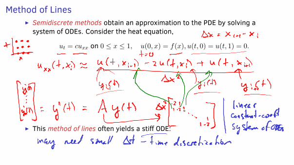
Method of Lines� Semidiscrete methods obtain an approximation to the PDE by solving a
system of ODEs. Consider the heat equation,
ut = cuxx on 0 ≤ x ≤ 1, u(0, x) = f(x), u(t, 0) = u(t, 1) = 0.
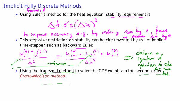
� This method of lines often yields a sti� ODE:
Semidiscrete Collocation� Instead of finite-di�erences, we can express u(t, x) in a spatial basis
� Consistency means that the local truncation error goes to zero, and is easy toverify by Taylor expansions.
� Stability implies that the approximate solution at any time t must remainbounded.
� Together these conditions are necessary and su�cient for convergence.
� Stability can be ascertained by spectral or Fourier analysis:
� In the method of lines, we saw that the eigenvalues of the resulting ODE definethe stability region.
� Fourier analysis decomposes the solution into a sum of harmonic functions andbounds their amplitudes.
CFL Condition� The domain of dependence of a PDE for a given point (t, x) is the portion of
the problem domain influencing this point through the PDE:
� The Courant, Friedrichs, and Lewy (CFL) condition states that a necessarycondition for an explicit finite-di�erencing scheme to be stable for ahyperbolic PDE is that the domain of the dependence of the PDE becontained in the domain of dependence of the scheme:
Time-Independent PDEs� We now turn our focus to time-independent PDEs as exemplified by the
Helmholtz equation:uxx + uyy + λu = f(x, y)
� We discretize as before, but no longer perform time stepping:
Finite-Di�erencing for Poisson� Consider the Poisson equation with equispaced mesh-points on [0, 1]:
Multidimensional Finite Elements� There are many ways to define localized basis functions, for example in the
2D FEM method2:
Sparse Linear Systems� Finite-di�erence and finite-element methods for time-independent PDEs give
rise to sparse linear systems:� typified by the 2D Laplace equation, where for both finite di�erences and FEM,
� Direct methods apply LU or other factorization to A, while iterative methodsrefine x by minimizing r = Ax− b, e.g. via Krylov subspace methods.
Direct Methods for Sparse Linear Systems� It helps to think of A as the adjacency matrix of graph G = (V,E) where
V = {1, . . . n} and aij �= 0 if and only if (i, j) ∈ E:
� Factorizing the lth row/column in Gaussian elimination corresponds toremoving node i, with nonzeros (new edges) introduces for each k, l suchthat (i, k) and (i, l) are in the graph.
Vertex Orderings for Direct Methods� Select the node of minimum degree at each step of factorization:
� Graph partitioning also serves to bound fill, remove vertex separator S ⊂ Vso that V \ S = V1 ∪ · · · ∪ Vk become disconnected, then order V1, . . . , Vk, S:
� Nested dissection ordering partitions graph into halves recursively, orderingeach separator last.
Demo: Sparse Matrix Factorizations and Fill-In
Sparse Iterative Methods
� Sparse iterative methods avoid overhead of fill in sparse direct factorization.Matrix splitting methods provide the most basic iterative methods:
Sparse Iterative Methods� The Jacobi method is the simplest iterative solver:
� The Jacobi method converges if A is strictly row-diagonally-dominant:
Gauss-Seidel Method� The Jacobi method takes weighted sums of x(k) to produce each entry of
x(k+1), while Gauss-Seidel uses the latest available values, i.e. to computex(k+1)i it uses a weighted sum of
x(k+1)1 , . . . x
(k+1)i−1 , x
(k)i , . . . , x(k)n .
� Gauss-Seidel provides somewhat better convergence than Jacobi:
Successive Over-Relaxation� The successive over-relaxation (SOR) method seeks to improve the spectral
radius achieved by Gauss-Seidel, by choosing
M =1
ωD +L, N =
� 1
ω− 1
�D −U
� The parameter ω in SOR controls the ‘step-size’ of the iterative method:
Demo: Stationary Iterative Methods
Conjugate Gradient� The solution to Ax = b is a minima of the quadratic optimization problem,
minx
||Ax− b||22
� Conjugate gradient works by picking A-orthogonal descent directions
� The convergence rate of CG is linear with coe�cient√
κ(A)−1√κ(A)+1
:
Demo: Jacobi vs Conjugate Gradient
Preconditioning� Preconditioning techniques choose matrix M ≈ A that is easy to invert and
solve a modified linear system with an equivalent solution to Ax = b,
M−1Ax = M−1b
� M is chosen to be an e�ective approximation to A with a simple structure: