28
CS1512 Foundations of Computing Science 2 Lecture 5 Inferential statistics
| Date post: | 28-Mar-2015 |
| Category: |
Documents |
| Upload: | colin-glass |
| View: | 224 times |
| Download: | 2 times |
CS1512Foundations ofComputing Science 2
Lecture 5
Inferential statistics
Originals from the University of San Diego, adapted by K.van Deemter
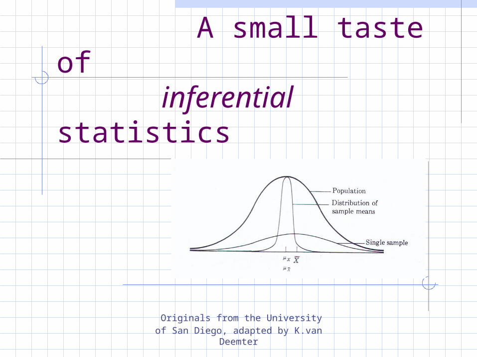
A small taste of inferential statistics
Reasons for sampling
If you want to know something about a population, your results would be most accurate if you could study the entire population.But it is often not feasible (cost, time) to study the whole population.
An example …
We suspect that there less crime in Aberdeen than the national average
How can we test this? We do not have the funds to
measure the crime rate in every street in Abdn, so we take a random sample of one or more streets.
An example ...
Sampling in general: Study a sample, and try to draw conclusions about the sample space (population) as a whole The larger the sample, the more accurately
will it tend to reflect the properties of the population
In this example: We calculate how much crime, on average, the streets in our sample have experienced and compare it to the national average.
1. A simplistic approach involving a sample of one
Suppose UK crime is normally distributed, with 4 crimes per street (mean ) and known st. dev. Now choose a sample of one Abdn street, which happens to have experienced 2 crimesSuppose Aberdeen crime levels were the same as the national average, how probable would it be to find 2 crimes or less crimes in a given street?Recall that this can be computed given mean and standard deviation of a normally distr. population.If this is highly unlikely then say “it looks as if Abdn has less crime than the national average”
But ...
National crime may not be normally distributedThe standard deviation on the number of crimes per street may be very high As a result of this, you may find that 2 or
less crimes per street may not be so improbable
For these reasons, a more sophisticated approach is called for The trick is to look at a larger sample and focus on the sample mean
2. A more sophisticated approach involving larger samples
What is the probability of obtaining the sample mean that you did? Compare your sample to other
samples of the same size from the same population.
To make calculations easy, suppose your variable can have values 2,4,6,8 only (e.g. two crimes, four crimes, etc). Consider all possible samples of two: {2,4}, {4,2},{2,6}, {6,2}, {4,4},...

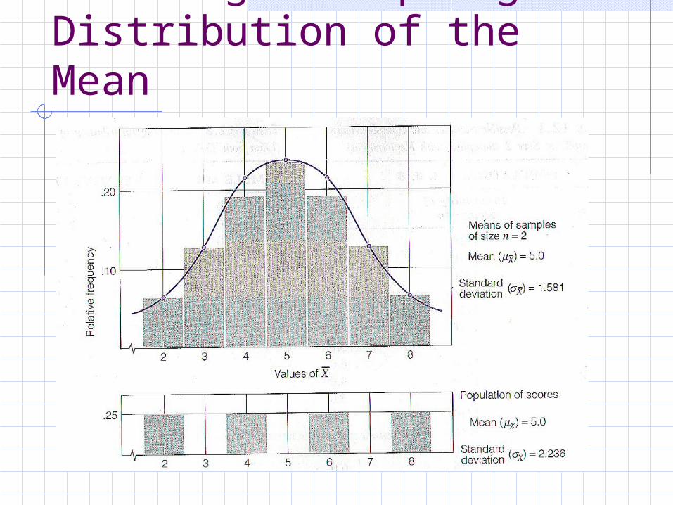
Creating a Sampling Distribution of the Mean
Although there are 16 different possible samples, there are not 16 different sample means possible. The ones that are possible have different probabilities.

The sampling distribution of the mean
Has the same mean as the original distribution Tends to be (almost) normally distributedHas a smaller standard deviationThe larger the sample size n, the smaller the standard deviation of the mean
x
nx
There is a formula which says how the new standard deviation depends on the old one () and the sample size n. In case you’re curious:
Creating a Sampling Distribution of the Mean
Sampling Distribution of the Mean
This distribution describes the entire spectrum of sample means that could occur just by chance.In other words, the sampling distribution of the mean allows us to determine whether, among the set of random possibilities, the one observed sample mean can be viewed as a common outcome or a rare outcome.

Using the Sampling Distribution of the Mean to Determine Probability
Probability of obtaining a particular sample mean.
Rare outcome.
Common outcome.
Rare outcome.

But we were not gambling on the likelihood that one particular sample mean will occur E.g., our guess was not: “average
crime in Aberdeen is 3 crimes per street”
Our guess was that crime in the average Aberdeen street was below the national average
How would statisticians handle this?

The correct procedure (just a sketch!)
We start with the hypothesis that the crime rate on average in Aberdeen is the same as the national average.
This is called the null Hypothesis (H0). This is roughly the opposite of what you try to confirm (which is called the alternative Hypothesis HA or the research Hypothesis): that there’s less crime in Aberdeen
To test the null hypothesis, we ask what sample means would occur if many samples of the same size were drawn at random from our population if our null hypothesis was true.
Then we compare our sample mean with the means in this sampling distribution.
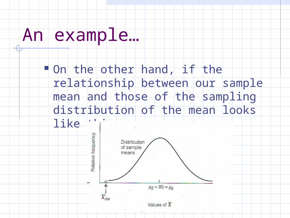
An example…
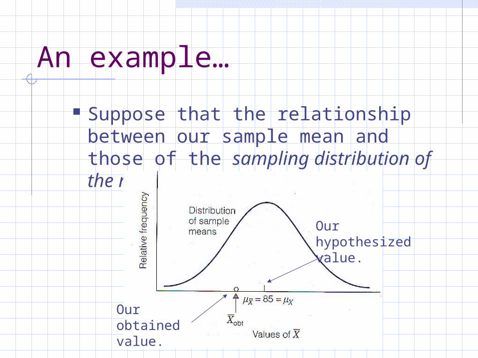
Suppose that the relationship between our sample mean and those of the sampling distribution of the mean looks like this…
Our obtained value.
Our hypothesized value.
An example…
If so, our sample mean is one that could reasonably occur if the null hypothesis is true, and we will retain this hypothesis as one that could be true. (i.e., The crime rate of Aberdeen could be the same as the national average.)
An example…
On the other hand, if the relationship between our sample mean and those of the sampling distribution of the mean looks like this…

An example…
Our sample mean is so deviant that it would be quite unusual to obtain such a value when our hypothesis is true. In this case, we would reject our hypothesis and conclude that it is more likely that the crime rate of Abdn is not the same as the national average. The population represented by the
sample differs significantly from the comparison population.

Going into this a bit more deeply (no need to understand this in detail)
But how deviant is deviant enough? In other words, How unlikely does H0 need to be to count as false?
In some areas a probability of 0.5 is generally agreed to be small enough ( 95% certainty)
In areas where errors are costly (e.g., medicine), it’s often chosen as low as 0.1 ( 99% certainty)
This is called the decision rule.We say that the difference between observed mean m and the hypothesised mean is significant if the decision rule decides that m is unlikely to have come about by accident.
0.1, 0.5, etc. are also called levels of significance
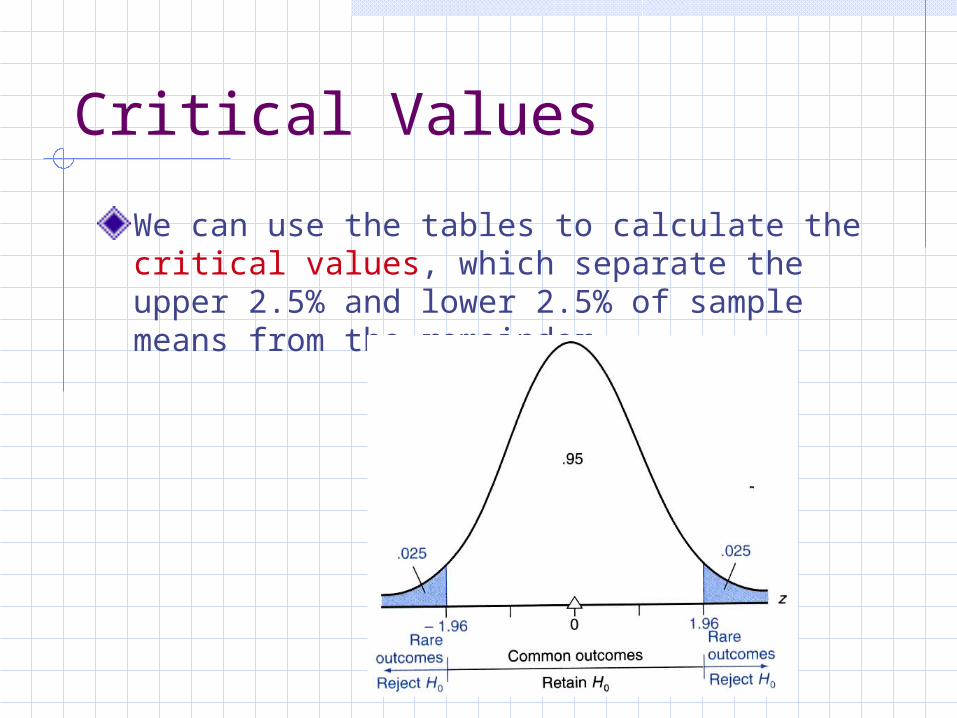
Critical Values
We can use the tables to calculate the critical values, which separate the upper 2.5% and lower 2.5% of sample means from the remainder.
Another example…
A psychologist is working with people who have had surgery. The psychologist thinks that people may recover from the operation more quickly if friends and family are in the room with them after the operation.
It is known that time to recover from this kind of surgery is normally distributed with a mean of 12 days and a standard deviation of 5 days.
The procedure of having friends and family in the room for the period after the surgery is done with 9 randomly selected patients. The patients recover in an average of 8 days.
Using the .01 level of significance, what should the researcher conclude?
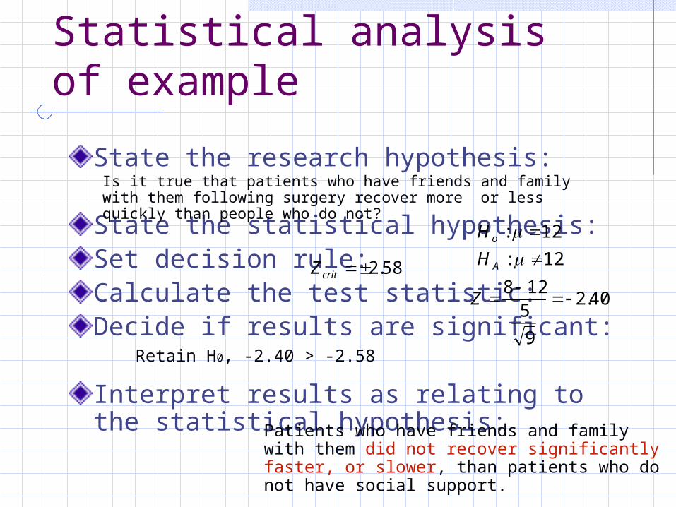
Statistical analysis of example
For illustration, we show here how this experiment is analysed statistically.
H0 is the null hypothesis HA is the alternative hypothesis (research hyp.)
A test statistic says how far from the population mean the sample mean is. An often-used statistic is ZZ involves the sample mean m, the hypothesised mean , and the standard deviation on the means

Statistical analysis of example
An often-used test statistic is Z. Z involves the sample mean m, the hypothesised mean , and the standard deviation on the means
We have seen that the standard deviation on the means is
n
mZ
nx
• The formula for Z is• Z = the difference between m and , compared with the new standard deviation
Statistical analysis of example
State the research hypothesis:
State the statistical hypothesis:Set decision rule:Calculate the test statistic:Decide if results are significant:
Interpret results as relating to the statistical hypothesis:
12:
12:
A
o
H
H
58.2critZ
40.2
9
5128
Z
Is it true that patients who have friends and family with them following surgery recover more or less quickly than people who do not?
Patients who have friends and family with them did not recover significantly faster, or slower, than patients who do not have social support.
Retain H0, -2.40 > -2.58
Does it follow that “friends and family do not have the predicted effect”?No! You may have used too few subjects, for example. The facts did point in the right direction (because recovery was 4 days faster, on average), so maybe do a bigger experiment
An experiment can never confirm the null hypothesis, only disconfirm it.

Summing up inferential statistics
This is essentially what’s been done when you read that one medicine is more effective than another one user interface is better liked than another one computer program runs faster than another,
on typical input In most cases, people are comparing one
sample with another (rather than with a completely known population, as in our examples)
Still, the techniques are always similar.

Summing up statistics and probability
We’ve covered some key concepts only (plus a quick illustration of how these concepts can be used in hypothesis testing) More from Professor Hunter, who will talk about
simulations and random number generators More in year 2, when you learn about HCI
In the lectures on probability, we wrote “P(q) = a”, where 0 <= a <= 1
Now we move on to Symbolic Logic, where we focus on the cases where a=0 or a=1


