CS208: Applied Privacy for Data ScienceMachine Learning under DP: Lecture

James Honaker & Salil VadhanSchool of Engineering & Applied Sciences

Harvard University

April 8, 2019

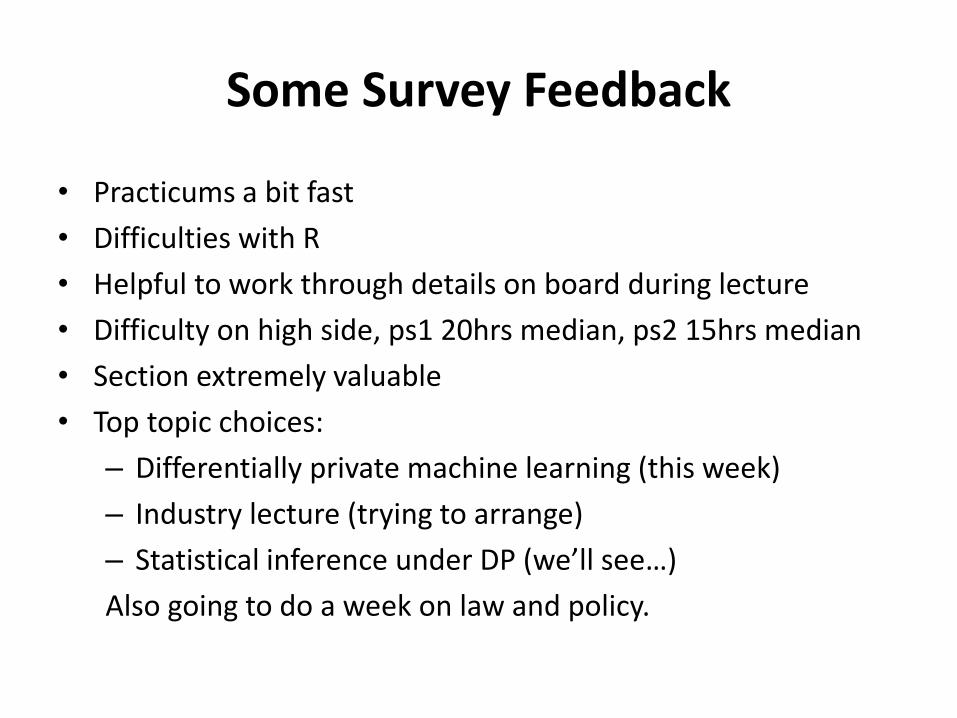
Some Survey Feedback

• Practicums a bit fast• Difficulties with R• Helpful to work through details on board during lecture• Difficulty on high side, ps1 20hrs median, ps2 15hrs median• Section extremely valuable• Top topic choices:

– Differentially private machine learning (this week)– Industry lecture (trying to arrange)– Statistical inference under DP (we’ll see…)Also going to do a week on law and policy.

Supervised ML Inputs

• Data 𝑥𝑥1,𝑦𝑦1 , … , 𝑥𝑥𝑛𝑛,𝑦𝑦𝑛𝑛 ∼ 𝒫𝒫– Examples 𝑥𝑥𝑖𝑖 ∈ 𝒳𝒳 𝑑𝑑-dimensional, discrete or continuous– Labels 𝑦𝑦𝑖𝑖 ∈ 𝒴𝒴 1-dimensional, discrete or continuous– 𝒫𝒫 typically unknown

• A family ℳ of models 𝑚𝑚𝜃𝜃: 𝒳𝒳 → 𝒴𝒴– Parameters 𝜃𝜃 ∈ Θ are 𝑘𝑘-dimensional, discrete or continuous– Linear regression: 𝑚𝑚𝛽𝛽,𝛼𝛼 𝑥𝑥 = 𝛽𝛽, 𝑥𝑥 + 𝛼𝛼

or 𝑚𝑚𝛽𝛽,𝛼𝛼,𝜎𝜎 𝑥𝑥 = 𝛽𝛽, 𝑥𝑥 + 𝛼𝛼 + 𝒩𝒩(0,𝜎𝜎2).– Deep neural nets: 𝜃𝜃 = vector of weights at all nodes

• A loss function ℓ ∶ Θ × 𝒳𝒳 × 𝒴𝒴 → ℝ– Classification error: ℓ 𝜃𝜃|𝑥𝑥,𝑦𝑦 = 𝐼𝐼(𝑚𝑚𝜃𝜃 𝑥𝑥 ≠ 𝑦𝑦).– Squared loss: ℓ 𝜃𝜃|𝑥𝑥,𝑦𝑦 = 𝑚𝑚𝜃𝜃 𝑥𝑥 − 𝑦𝑦 2.– Negative Log-likelihood: ℓ 𝜃𝜃|𝑥𝑥,𝑦𝑦 = −log Pr

𝑚𝑚[𝑚𝑚𝜃𝜃 𝑦𝑦 = 𝑥𝑥]

Supervised ML Output

Primary Goal (risk minimization):• Find 𝜃𝜃 ∈ Θ minimizing 𝐿𝐿 𝜃𝜃 = E 𝑥𝑥,𝑦𝑦 ∼𝒫𝒫 ℓ(𝜃𝜃|𝑥𝑥,𝑦𝑦) .• Difficulty: 𝒫𝒫 unknown.

Subgoal 1 (empirical risk minimization (ERM)):• Find 𝜃𝜃 ∈ Θ minimizing 𝐿𝐿 𝜃𝜃|�⃗�𝑥, �⃗�𝑦 = 1

𝑛𝑛∑𝑖𝑖=1𝑛𝑛 ℓ(𝜃𝜃|𝑥𝑥𝑖𝑖 ,𝑦𝑦𝑖𝑖) .

• Turns learning into optimization.• Difficulty: overfitting*

Subgoal 2 (regularized ERM):• Find 𝜃𝜃 ∈ Θ minimizing 𝐿𝐿 𝜃𝜃|�⃗�𝑥, �⃗�𝑦 = 1

𝑛𝑛∑𝑖𝑖=1𝑛𝑛 ℓ(𝜃𝜃|𝑥𝑥𝑖𝑖 ,𝑦𝑦𝑖𝑖) + 𝑅𝑅 𝜃𝜃 .

• 𝑅𝑅(𝜃𝜃) typically penalizes “large” 𝜃𝜃, can capture Bayesian prior.

*Fact: DP automatically helps prevent overfitting! [Dwork et al. `15]

APPROACHES TO ML WITH DP

Output Perturbation[Chaudhuri-Monteleoni-Sarwate `11]

𝑀𝑀 �⃗�𝑥, �⃗�𝑦 = argmin𝜃𝜃1𝑛𝑛�𝑖𝑖=1

𝑛𝑛

ℓ(𝜃𝜃|𝑥𝑥𝑖𝑖 ,𝑦𝑦𝑖𝑖) + 𝑅𝑅 𝜃𝜃 + Noise

Challenge: bounding sensitivity of 𝜃𝜃𝑜𝑜𝑜𝑜𝑜𝑜 = argmin𝜃𝜃 ⋅• Global sensitivity can be infinite (e.g. OLS regression)• Global sensitivity can be bounded when ℓ is strictly convex, has

bounded gradient (as a function of 𝜃𝜃), and 𝑅𝑅 is strongly convex. Even analyzing local sensitivity seems to require unique global optimum and using an optimizer that is guaranteed to succeed.

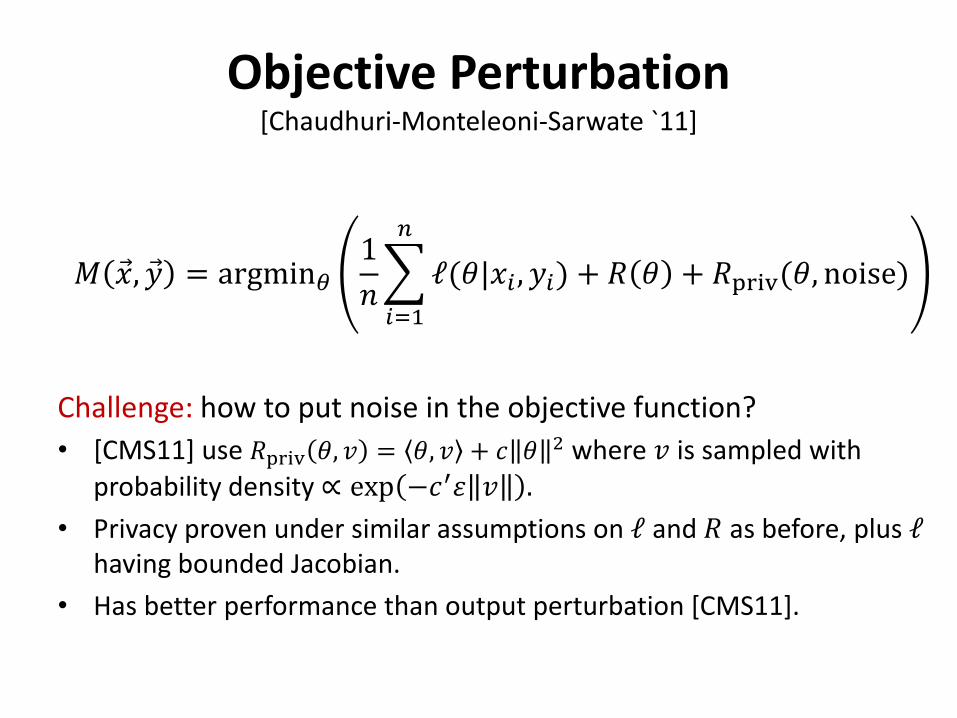
Objective Perturbation[Chaudhuri-Monteleoni-Sarwate `11]

𝑀𝑀 �⃗�𝑥, �⃗�𝑦 = argmin𝜃𝜃1𝑛𝑛�𝑖𝑖=1

𝑛𝑛

ℓ(𝜃𝜃|𝑥𝑥𝑖𝑖 ,𝑦𝑦𝑖𝑖) + 𝑅𝑅 𝜃𝜃 + 𝑅𝑅priv(𝜃𝜃, noise)

Challenge: how to put noise in the objective function?• [CMS11] use 𝑅𝑅priv 𝜃𝜃, 𝑣𝑣 = 𝜃𝜃, 𝑣𝑣 + 𝑐𝑐 𝜃𝜃 2 where 𝑣𝑣 is sampled with

probability density ∝ exp −𝑐𝑐′𝜀𝜀 𝑣𝑣 .• Privacy proven under similar assumptions on ℓ and 𝑅𝑅 as before, plus ℓ

having bounded Jacobian.• Has better performance than output perturbation [CMS11].

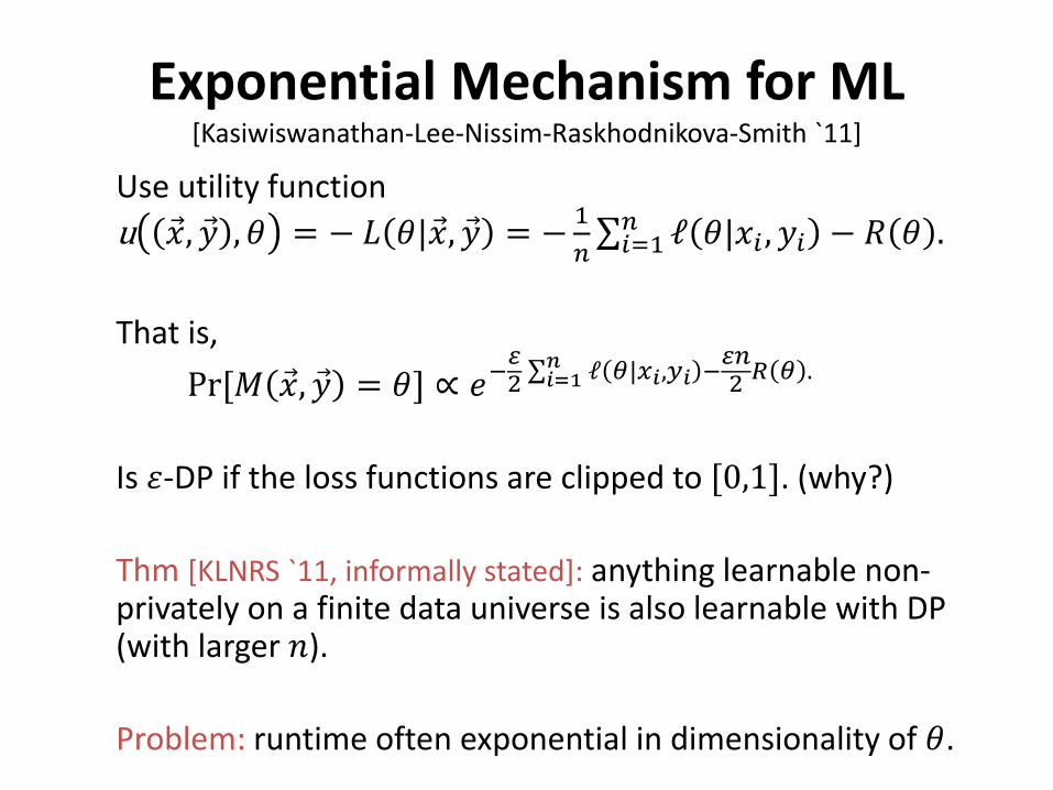
Exponential Mechanism for ML[Kasiwiswanathan-Lee-Nissim-Raskhodnikova-Smith `11]

Use utility function u �⃗�𝑥, �⃗�𝑦 ,𝜃𝜃 = − 𝐿𝐿 𝜃𝜃|�⃗�𝑥, �⃗�𝑦 = − 1

𝑛𝑛∑𝑖𝑖=1𝑛𝑛 ℓ 𝜃𝜃|𝑥𝑥𝑖𝑖 ,𝑦𝑦𝑖𝑖 − 𝑅𝑅 𝜃𝜃 .

That is, Pr[𝑀𝑀 �⃗�𝑥, �⃗�𝑦 = 𝜃𝜃] ∝ 𝑒𝑒−

𝜀𝜀2 ∑𝑖𝑖=1

𝑛𝑛 ℓ 𝜃𝜃|𝑥𝑥𝑖𝑖,𝑦𝑦𝑖𝑖 −𝜀𝜀𝑛𝑛2 𝑅𝑅 𝜃𝜃 .

Is 𝜀𝜀-DP if the loss functions are clipped to [0,1]. (why?)

Thm [KLNRS `11, informally stated]: anything learnable non-privately on a finite data universe is also learnable with DP (with larger 𝑛𝑛).

Problem: runtime often exponential in dimensionality of 𝜃𝜃.

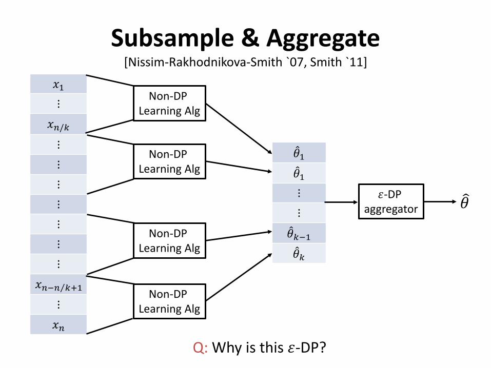
Subsample & Aggregate[Nissim-Rakhodnikova-Smith `07, Smith `11]

𝑥𝑥1⋮

𝑥𝑥𝑛𝑛/𝑘𝑘

⋮⋮⋮⋮⋮⋮⋮

𝑥𝑥𝑛𝑛− ⁄𝑛𝑛 𝑘𝑘+1

⋮𝑥𝑥𝑛𝑛

Non-DP Learning Alg

Non-DP Learning Alg

Non-DP Learning Alg

Non-DP Learning Alg

�̂�𝜃1�̂�𝜃1⋮⋮

�̂�𝜃𝑘𝑘−1�̂�𝜃𝑘𝑘

𝜀𝜀-DP aggregator

�𝜃𝜃

Q: Why is this 𝜀𝜀-DP?

Subsample & Aggregate[Nissim-Rakhodnikova-Smith `07, Smith `11]

• Typical aggregators: DP (clipped) mean, DP median• Benefits:

– Use any non-private estimator as a black box– Can give optimal asymptotic convergence rates: for many statistical

estimators, variance is asymptotically 𝑐𝑐𝜃𝜃/(sample size), so variance of DP mean �̂�𝜃 is

( ⁄1 𝑘𝑘) ⋅ 𝑐𝑐𝜃𝜃 ⋅ ⁄𝑘𝑘 𝑛𝑛 + 𝑂𝑂( ⁄1 𝜀𝜀𝑘𝑘)2 = 1 + 𝑜𝑜 1 ⋅ 𝑐𝑐𝜃𝜃/𝑛𝑛if 𝑘𝑘 = 𝜔𝜔 𝑛𝑛 .

• Drawbacks:– Dependence on dimension, model parameters, distribution can be bad.– Often takes very large sample size to kick in.

Modifying ML Algorithms

• Another approach: decompose existing ML/inference algorithms into steps that can be made DP, like Statistical Queries (estimating means of bounded functions)

• Example: linear regression– ⁄𝑆𝑆𝑥𝑥𝑥𝑥 𝑛𝑛 , ⁄𝑆𝑆𝑥𝑥𝑦𝑦 𝑛𝑛 , �̅�𝑥, �𝑦𝑦 are all statistical queries

• Today: gradient descent and variants– main method used in practice for training deep neural nets

GRADIENT DESCENT WITH DP(slides modified from Adam Smith, BU CS 591 Fall 2018)

Gradient Descent• Proceed in steps

• Start from (carefully chosen) initial parameters �̂�𝜃0• At each step, move in direction opposite to the

gradient of the loss ∇𝐿𝐿(�̂�𝜃│�⃗�𝑥, �⃗�𝑦).• Gradient is the vector of partial derivatives

[Wikipedia]

Gradient Descent for Convex Loss

18

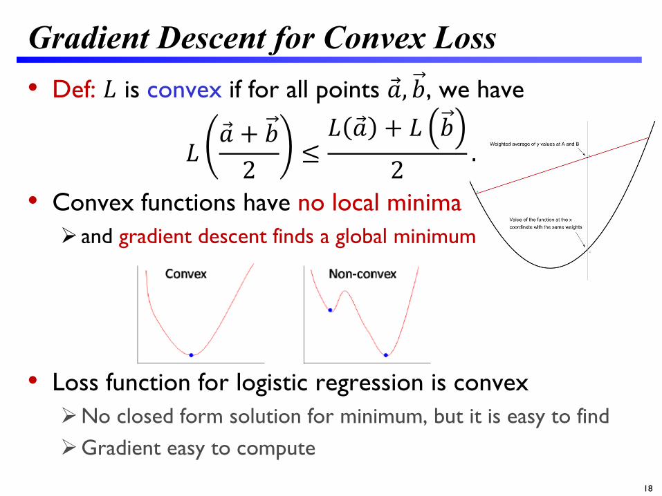
• Def: 𝐿𝐿 is convex if for all points �⃗�𝑎, 𝑏𝑏, we have

𝐿𝐿�⃗�𝑎 + 𝑏𝑏

2≤𝐿𝐿 �⃗�𝑎 + 𝐿𝐿 𝑏𝑏

2.

• Convex functions have no local minima and gradient descent finds a global minimum

• Loss function for logistic regression is convexNo closed form solution for minimum, but it is easy to findGradient easy to compute

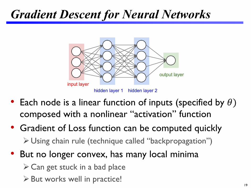
Gradient Descent for Neural Networks

• Each node is a linear function of inputs (specified by 𝜃𝜃)composed with a nonlinear “activation” function

• Gradient of Loss function can be computed quicklyUsing chain rule (technique called “backpropagation”)

• But no longer convex, has many local minimaCan get stuck in a bad placeBut works well in practice!

19

Common activation functions

20

Sigmoid 𝜎𝜎 𝑥𝑥 = 11+𝑒𝑒−𝑥𝑥 tanh 𝑥𝑥 = 2𝜎𝜎 2𝑥𝑥 − 1

ReLU 𝑥𝑥 = max(0, 𝑥𝑥) Leaky ReLU 𝑥𝑥 = max(0.05𝑥𝑥, 𝑥𝑥)

Neural Networks & Privacy• Best known models for many problems are DNNs

Sentence prediction (smart completion) Image/video/text recognition Author recognition Textual analysis …

• Problem: The best DNNs end up memorizing their inputs! Chiyuan Zhang, Samy Bengio, Moritz Hardt, Benjamin Recht, and Oriol

Vinyals. Understanding deep learning requires rethinking generalization. International Conference on Learning Representations (ICLR), 2017.

Nicholas Carlini, Chang Liu, Jernej Kos, Úlfar Erlingsson, Dawn Song. The Secret Sharer: Measuring Unintended Neural Network Memorization & Extracting Secrets. arXiv:1802.08232

• Potential solution Differentially private training of DNNs Input: training data Output: architecture & weights

21

Gradient Descent: Formal Description

22

• SpecifyNumber of steps 𝑇𝑇Learning rate 𝜂𝜂

• Pick initial point �̂�𝜃0• For 𝑡𝑡 = 1 to 𝑇𝑇Compute gradient

𝑔𝑔𝑜𝑜 =1𝑛𝑛�𝑖𝑖

∇ℓ �𝜃𝜃𝑜𝑜−1|𝑥𝑥𝑖𝑖 ,𝑦𝑦𝑖𝑖 + ∇𝑅𝑅 �𝜃𝜃𝑜𝑜−1

�𝜃𝜃𝑜𝑜 = �𝜃𝜃𝑜𝑜−1 − 𝜂𝜂 ⋅ 𝑔𝑔𝑜𝑜

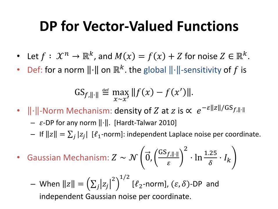
DP for Vector-Valued Functions

• Let 𝑓𝑓 ∶ 𝒳𝒳𝑛𝑛 → ℝ𝑘𝑘, and 𝑀𝑀 𝑥𝑥 = 𝑓𝑓 𝑥𝑥 + 𝑍𝑍 for noise 𝑍𝑍 ∈ ℝ𝑘𝑘.• Def: for a norm ⋅ on ℝ𝑘𝑘. the global ⋅ -sensitivity of 𝑓𝑓 is

GS𝑓𝑓, ⋅ ≝ max𝑥𝑥∼𝑥𝑥′

𝑓𝑓 𝑥𝑥 − 𝑓𝑓 𝑥𝑥′ .

• ⋅ -Norm Mechanism: density of 𝑍𝑍 at 𝑧𝑧 is ∝ 𝑒𝑒−𝜀𝜀 𝑧𝑧 /GS𝑓𝑓, ⋅

– 𝜀𝜀-DP for any norm ⋅ . [Hardt-Talwar 2010]– If 𝑧𝑧 = ∑𝑗𝑗 |𝑧𝑧𝑗𝑗| [ℓ1-norm]: independent Laplace noise per coordinate.

• Gaussian Mechanism: 𝑍𝑍 ∼ 𝒩𝒩 0,GS𝑓𝑓, ⋅

𝜀𝜀

2⋅ ln 1.25

𝛿𝛿⋅ 𝐼𝐼𝑘𝑘

– When 𝑧𝑧 = ∑𝑗𝑗 𝑧𝑧𝑗𝑗2 1/2

[ℓ2-norm], (𝜀𝜀, 𝛿𝛿)-DP and independent Gaussian noise per coordinate.

DP Gradient Descent

24

[Williams-McSherry`10, …]

• SpecifyNumber of steps 𝑇𝑇Learning rate 𝜂𝜂Privacy parameters 𝜀𝜀, 𝛿𝛿

Clipping parameter ∆. Write 𝑧𝑧 ∆ = 𝑧𝑧 ⋅ max 1, ∆𝑧𝑧 2

.

Noise variance 𝜎𝜎2 = TBD(𝑇𝑇, 𝜀𝜀, 𝛿𝛿,∆).

• Pick initial point �̂�𝜃0• For 𝑡𝑡 = 1 to 𝑇𝑇Estimate gradient as noisy average of clipped gradients �𝑔𝑔𝑜𝑜 = 1

𝑛𝑛∑𝑖𝑖 ∇ℓ �𝜃𝜃𝑜𝑜−1|𝑥𝑥𝑖𝑖 ,𝑦𝑦𝑖𝑖 ∆ + ∇𝑅𝑅 �𝜃𝜃𝑜𝑜−1 + 𝒩𝒩(0,𝜎𝜎2𝐼𝐼)

�𝜃𝜃𝑜𝑜 = �𝜃𝜃𝑜𝑜−1 − 𝜂𝜂 ⋅ �𝑔𝑔𝑜𝑜

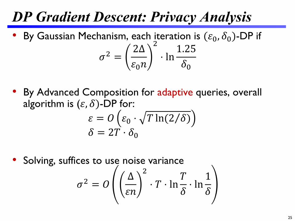
DP Gradient Descent: Privacy Analysis

25

• By Gaussian Mechanism, each iteration is (𝜀𝜀0, 𝛿𝛿0)-DP if

𝜎𝜎2 =2∆𝜀𝜀0𝑛𝑛

2

⋅ ln1.25𝛿𝛿0

• By Advanced Composition for adaptive queries, overall algorithm is (𝜀𝜀, 𝛿𝛿)-DP for:

𝜀𝜀 = 𝑂𝑂 𝜀𝜀0 ⋅ 𝑇𝑇 ln( ⁄2 𝛿𝛿)𝛿𝛿 = 2𝑇𝑇 ⋅ 𝛿𝛿0

• Solving, suffices to use noise variance

𝜎𝜎2 = 𝑂𝑂∆𝜀𝜀𝑛𝑛

2

⋅ 𝑇𝑇 ⋅ ln𝑇𝑇𝛿𝛿⋅ ln

1𝛿𝛿

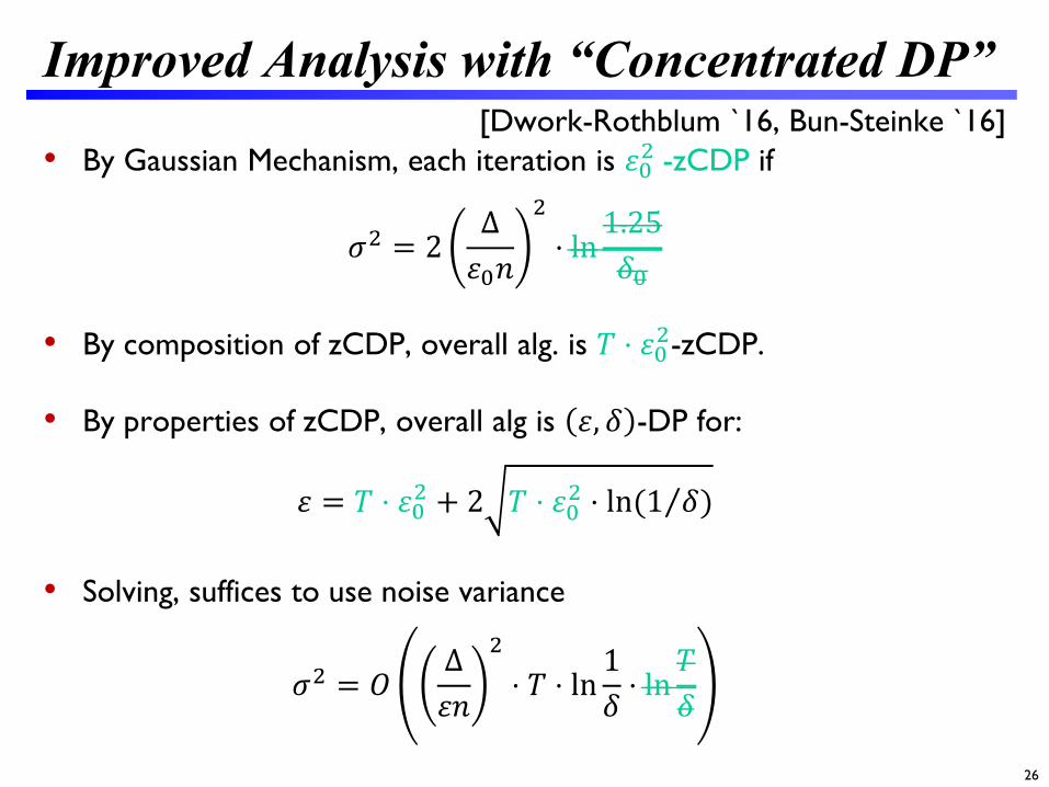
Improved Analysis with “Concentrated DP”

26

[Dwork-Rothblum `16, Bun-Steinke `16]• By Gaussian Mechanism, each iteration is 𝜀𝜀02 -zCDP if

𝜎𝜎2 = 2∆𝜀𝜀0𝑛𝑛

2

⋅ ln1.25𝛿𝛿0

• By composition of zCDP, overall alg. is 𝑇𝑇 ⋅ 𝜀𝜀02-zCDP.

• By properties of zCDP, overall alg is 𝜀𝜀, 𝛿𝛿 -DP for:

𝜀𝜀 = 𝑇𝑇 ⋅ 𝜀𝜀02 + 2 𝑇𝑇 ⋅ 𝜀𝜀02 ⋅ ln( ⁄1 𝛿𝛿)

• Solving, suffices to use noise variance

𝜎𝜎2 = 𝑂𝑂∆𝜀𝜀𝑛𝑛

2

⋅ 𝑇𝑇 ⋅ ln1𝛿𝛿⋅ ln

𝑇𝑇𝛿𝛿

DP Stochastic Gradient Descent (SGD)

27

[Jain-Kothari-Thakurta `12, Song-Chaudhuri-Sarwate `13, Bassily-Smith-Thakurta `14]

• Specify Number of steps 𝑇𝑇, learning rate 𝜂𝜂, privacy parameters 𝜀𝜀, 𝛿𝛿, clipping

parameter ∆. Batch size 𝐵𝐵 ≪ 𝑛𝑛 (for efficiency) Noise variance 𝜎𝜎2 = TBD(𝑇𝑇, 𝜀𝜀, 𝛿𝛿,∆,𝐵𝐵).

• Pick initial point �̂�𝜃0• For 𝑡𝑡 = 1 to 𝑇𝑇 Select a random batch 𝑆𝑆𝑜𝑜 ⊆ {1, … ,𝑛𝑛} of size 𝐵𝐵.Estimate gradient as noisy average of clipped gradients �𝑔𝑔𝑜𝑜 = 1

𝐵𝐵∑𝑖𝑖∈𝑆𝑆𝑡𝑡 ∇ℓ �𝜃𝜃𝑜𝑜−1|𝑥𝑥𝑖𝑖 ,𝑦𝑦𝑖𝑖 ∆ + ∇𝑅𝑅 �𝜃𝜃𝑜𝑜−1 + 𝒩𝒩(0,𝜎𝜎2𝐼𝐼)

�𝜃𝜃𝑜𝑜 = �𝜃𝜃𝑜𝑜−1 − 𝜂𝜂 ⋅ �𝑔𝑔𝑜𝑜

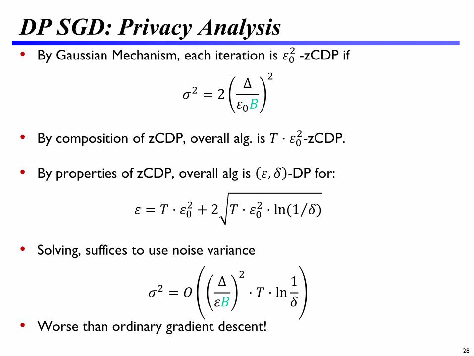
DP SGD: Privacy Analysis

28

• By Gaussian Mechanism, each iteration is 𝜀𝜀02 -zCDP if

𝜎𝜎2 = 2∆𝜀𝜀0𝐵𝐵

2

• By composition of zCDP, overall alg. is 𝑇𝑇 ⋅ 𝜀𝜀02-zCDP.

• By properties of zCDP, overall alg is 𝜀𝜀, 𝛿𝛿 -DP for:

𝜀𝜀 = 𝑇𝑇 ⋅ 𝜀𝜀02 + 2 𝑇𝑇 ⋅ 𝜀𝜀02 ⋅ ln( ⁄1 𝛿𝛿)

• Solving, suffices to use noise variance

𝜎𝜎2 = 𝑂𝑂∆𝜀𝜀𝐵𝐵

2

⋅ 𝑇𝑇 ⋅ ln1𝛿𝛿

• Worse than ordinary gradient descent!

DP SGD: Improved Privacy Analysis

29

[Bassily-Smith-Thakurta `14, Abadi-Chu-Goodfellow-McMahan-Mironov-Talwar-Zhang `17]

• Privacy amplification by subsampling:If 𝑆𝑆 ∶ 𝒳𝒳𝑛𝑛 → 𝒳𝒳𝐵𝐵 outputs a random subset of 𝑝𝑝𝑛𝑛 out of 𝑛𝑛 rows and 𝑀𝑀 ∶ 𝒳𝒳𝐵𝐵 → 𝒴𝒴 is (𝜀𝜀, 𝛿𝛿)-DP, then 𝑀𝑀′ 𝑥𝑥 = 𝑀𝑀(𝑆𝑆 𝑥𝑥 ) is ( 𝑒𝑒𝑜𝑜 − 1 ⋅ 𝜀𝜀, 𝑝𝑝 ⋅ 𝛿𝛿)-DP.

• We can take 𝑝𝑝 = ⁄𝐵𝐵 𝑛𝑛 .Unfortunately does privacy amplification by subsampling does

not hold for zCDP.But similar analysis can be recovered using the “moments

accountant” [Abadi et al. `17] or “truncated zCDP” [Bun et al. `18].

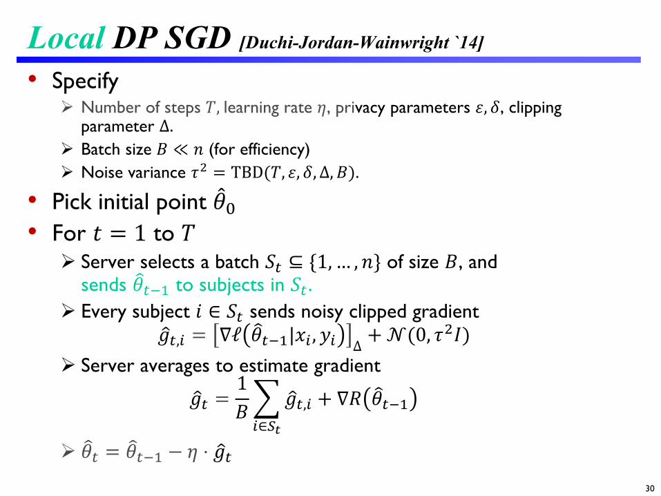
Local DP SGD [Duchi-Jordan-Wainwright `14]

30

• Specify Number of steps 𝑇𝑇, learning rate 𝜂𝜂, privacy parameters 𝜀𝜀, 𝛿𝛿, clipping

parameter ∆. Batch size 𝐵𝐵 ≪ 𝑛𝑛 (for efficiency) Noise variance 𝜏𝜏2 = TBD(𝑇𝑇, 𝜀𝜀, 𝛿𝛿,∆,𝐵𝐵).

• Pick initial point �̂�𝜃0• For 𝑡𝑡 = 1 to 𝑇𝑇 Server selects a batch 𝑆𝑆𝑜𝑜 ⊆ {1, … ,𝑛𝑛} of size 𝐵𝐵, and

sends �𝜃𝜃𝑜𝑜−1 to subjects in 𝑆𝑆𝑜𝑜. Every subject 𝑖𝑖 ∈ 𝑆𝑆𝑜𝑜 sends noisy clipped gradient

�𝑔𝑔𝑜𝑜,𝑖𝑖 = ∇ℓ �𝜃𝜃𝑜𝑜−1|𝑥𝑥𝑖𝑖 ,𝑦𝑦𝑖𝑖 ∆ + 𝒩𝒩(0, 𝜏𝜏2𝐼𝐼) Server averages to estimate gradient

�𝑔𝑔𝑜𝑜 =1𝐵𝐵�𝑖𝑖∈𝑆𝑆𝑡𝑡

�𝑔𝑔𝑜𝑜,𝑖𝑖 + ∇𝑅𝑅 �𝜃𝜃𝑜𝑜−1

�𝜃𝜃𝑜𝑜 = �𝜃𝜃𝑜𝑜−1 − 𝜂𝜂 ⋅ �𝑔𝑔𝑜𝑜

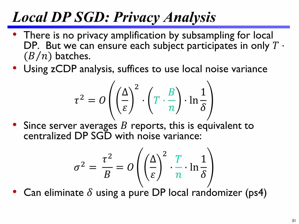
Local DP SGD: Privacy Analysis

31

• There is no privacy amplification by subsampling for local DP. But we can ensure each subject participates in only 𝑇𝑇 ⋅( ⁄𝐵𝐵 𝑛𝑛) batches.

• Using zCDP analysis, suffices to use local noise variance

𝜏𝜏2 = 𝑂𝑂∆𝜀𝜀

2

⋅ 𝑇𝑇 ⋅𝐵𝐵𝑛𝑛

⋅ ln1𝛿𝛿

• Since server averages 𝐵𝐵 reports, this is equivalent to centralized DP SGD with noise variance:

𝜎𝜎2 =𝜏𝜏2

𝐵𝐵= 𝑂𝑂

∆𝜀𝜀

2

⋅𝑇𝑇𝑛𝑛⋅ ln

1𝛿𝛿

• Can eliminate 𝛿𝛿 using a pure DP local randomizer (ps4)

Publicly available tools for DP Learning• Basic Mechanisms as building blocks (R): link• Techniques for DP Convex Optimization (Python): link• DP SGD (DNNs) using Tensorflow (Python): linkDP MNIST exampleDP Optimizer link

32

More on Non-DP Deep Learning• Stanford CS231n lecture notes

http://cs231n.github.io/neural-networks-1/• Deep learning tutorial

http://www.deeplearning.net/tutorial/mlp.html• TensorFlow visual demo

https://playground.tensorflow.org• Tensorflow and PyTorch tutorials

33