70
CS26007:Introduction to Wireless Networking Guangtao Xue Department of Computer Sciences, Shanghai Jiao Tong University Fall 2015

CS26007:Introduction to Wireless Networking
Guangtao XueDepartment of Computer Sciences,
Shanghai Jiao Tong University
Fall 2015
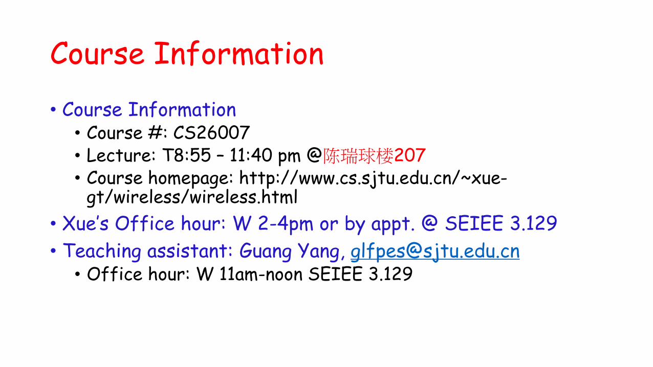
Course Information
• Course Information• Course #: CS26007• Lecture: T8:55 – 11:40 pm @陈瑞球楼207• Course homepage: http://www.cs.sjtu.edu.cn/~xue-
gt/wireless/wireless.html
• Xue’s Office hour: W 2-4pm or by appt. @ SEIEE 3.129
• Teaching assistant: Guang Yang, [email protected]• Office hour: W 11am-noon SEIEE 3.129

Course Workload
•Grading-Class participation: 20% (include in-class exercises)
-Homework: 30%
-Project: 50%
Course Material• Required textbook
– Ad Hoc Wireless Networks: Architectures and Protocols by C. Siva Ram Murthy and B.S. Manoj– Mobile Communications by Jochen Schiller
• Recommended references– Computer Networking: A top down approach featuring the Internet by James Kurose and Keith Ross– 802.11 Wireless Networks: The Definitive Guide by Matthew S. Gast– Wireless Communications Principles and Practice by Ted Rappaport– Ad Hoc Networking by Charles E. Perkins

Motivation

UMTS,
DECT
2 Mbit/s
UMTS, GSM
384 kbit/s
UMTS, GSM
115 kbit/s
GSM 115 kbit/s,
WLAN 11 Mbit/s
GSM 53 kbit/s
Bluetooth 500 kbit/s
GSM/EDGE 384 kbit/s,
WLAN 780 kbit/s
LAN, WLAN
600 Mbps
Mobile and Wireless Services –Always Best Connected
100kps

On the road

UMTS, WLAN,
DAB, GSM, WiMAX, LTE
cdma2000, TETRA, ...
GPS, GSM, WLAN, Bluetooth,
Ad hoc networks
On the Road

Home Networking
Camcorder
HDTV
Game
Game
iPod
High-quality
speaker
UWB
WiFi Bluetooth
WiFi
Surveillance
Surveillance
Surveillance
WiFi
WiFi
GSM, LTE,WiMAX
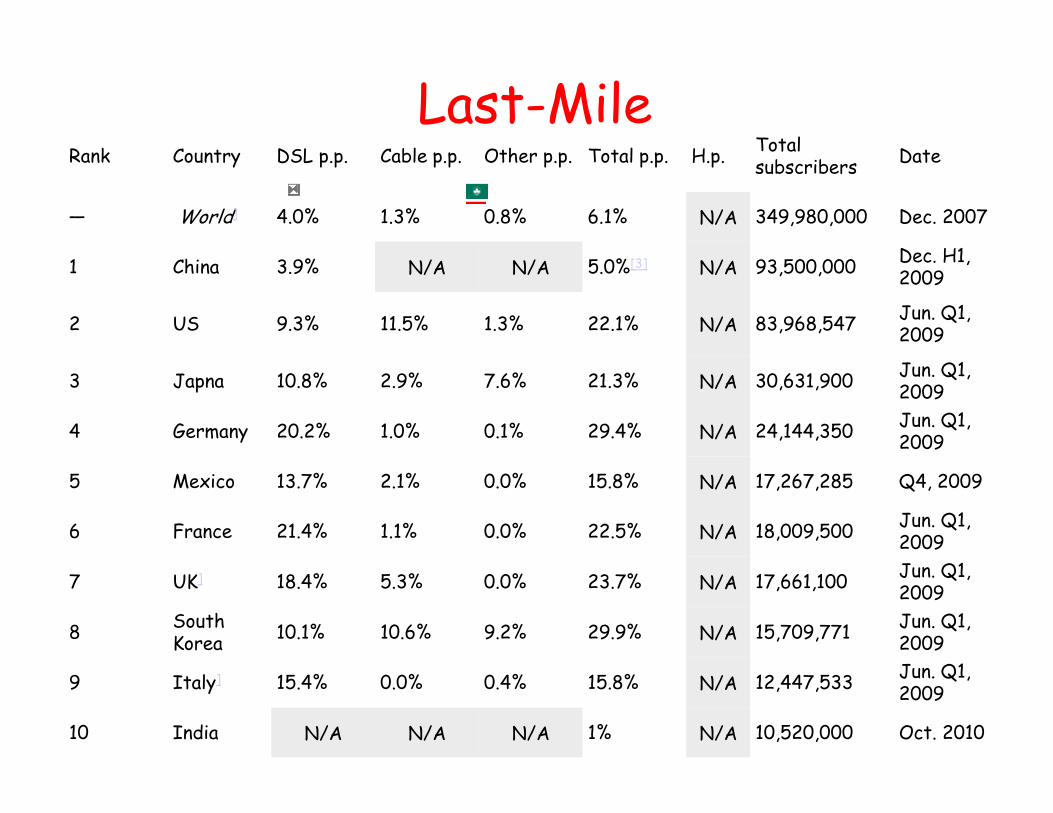
Last-MileRank Country DSL p.p. Cable p.p. Other p.p. Total p.p. H.p.
Total subscribers
Date
— World] 4.0% 1.3% 0.8% 6.1% N/A 349,980,000 Dec. 2007
1 China 3.9% N/A N/A 5.0%[3] N/A 93,500,000Dec. H1, 2009
2 US 9.3% 11.5% 1.3% 22.1% N/A 83,968,547Jun. Q1, 2009
3 Japna 10.8% 2.9% 7.6% 21.3% N/A 30,631,900Jun. Q1, 2009
4 Germany 20.2% 1.0% 0.1% 29.4% N/A 24,144,350Jun. Q1, 2009
5 Mexico 13.7% 2.1% 0.0% 15.8% N/A 17,267,285 Q4, 2009
6 France 21.4% 1.1% 0.0% 22.5% N/A 18,009,500Jun. Q1, 2009
7 UK] 18.4% 5.3% 0.0% 23.7% N/A 17,661,100Jun. Q1, 2009
8South Korea
10.1% 10.6% 9.2% 29.9% N/A 15,709,771Jun. Q1, 2009
9 Italy] 15.4% 0.0% 0.4% 15.8% N/A 12,447,533Jun. Q1, 2009
10 India N/A N/A N/A 1% N/A 10,520,000 Oct. 2010
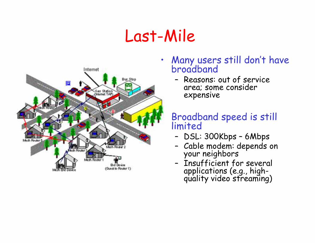
Last-Mile• Many users still don’t have
broadband– Reasons: out of service
area; some consider expensive
• Broadband speed is still limited– DSL: 300Kbps – 6Mbps– Cable modem: depends on
your neighbors– Insufficient for several
applications (e.g., high-quality video streaming)
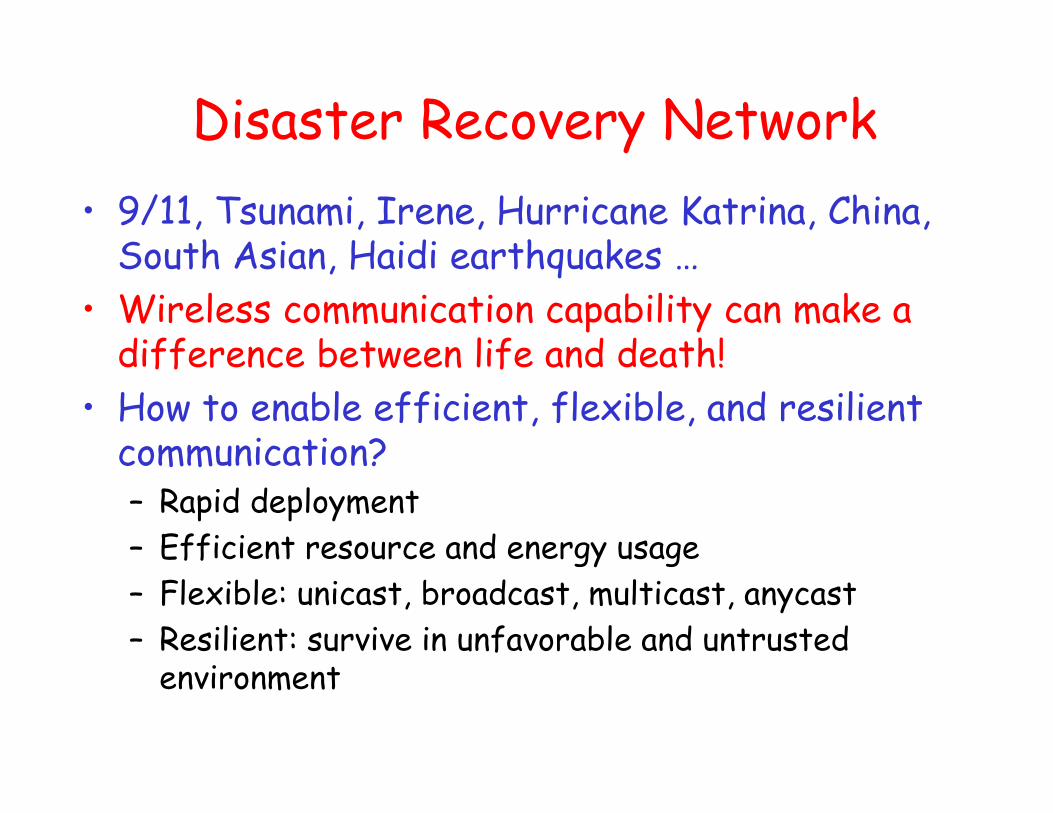
Disaster Recovery Network
• 9/11, Tsunami, Irene, Hurricane Katrina, China, South Asian, Haidi earthquakes …
• Wireless communication capability can make a difference between life and death!
• How to enable efficient, flexible, and resilient communication?– Rapid deployment
– Efficient resource and energy usage
– Flexible: unicast, broadcast, multicast, anycast
– Resilient: survive in unfavorable and untrusted environment

• Micro-sensors, on-board processing, wireless interfaces feasible at very small scale--can monitor phenomena “up close”
• Enables spatially and temporally dense environmental monitoring
Embedded Networked Sensing will reveal
previously unobservable phenomena
Contaminant TransportEcosystems, Biocomplexity
Marine Microorganisms Seismic Structure Response
Environmental Monitoring

Wearable Computing

Challenges in Wireless Networking Research
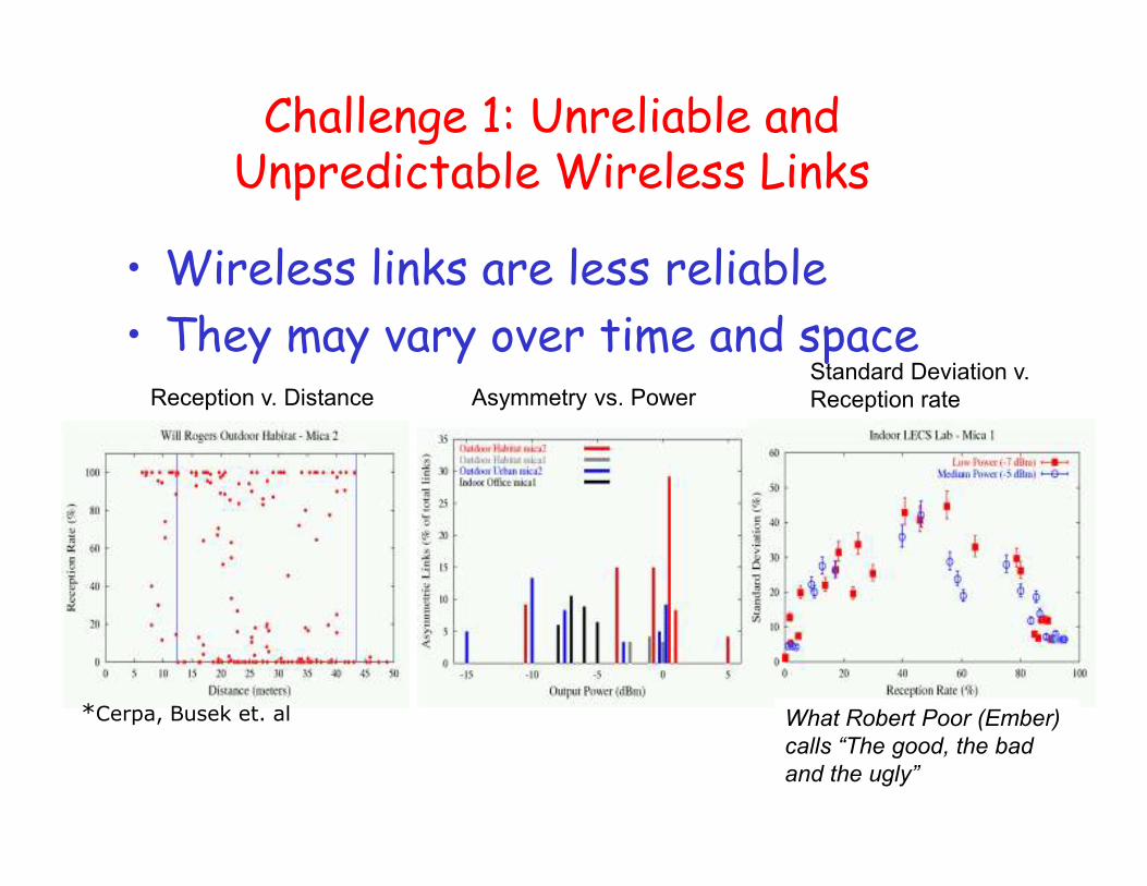
Challenge 1: Unreliable and Unpredictable Wireless Links
Asymmetry vs. PowerReception v. DistanceStandard Deviation v.
Reception rate
*Cerpa, Busek et. al What Robert Poor (Ember)
calls “The good, the bad
and the ugly”
• Wireless links are less reliable
• They may vary over time and space

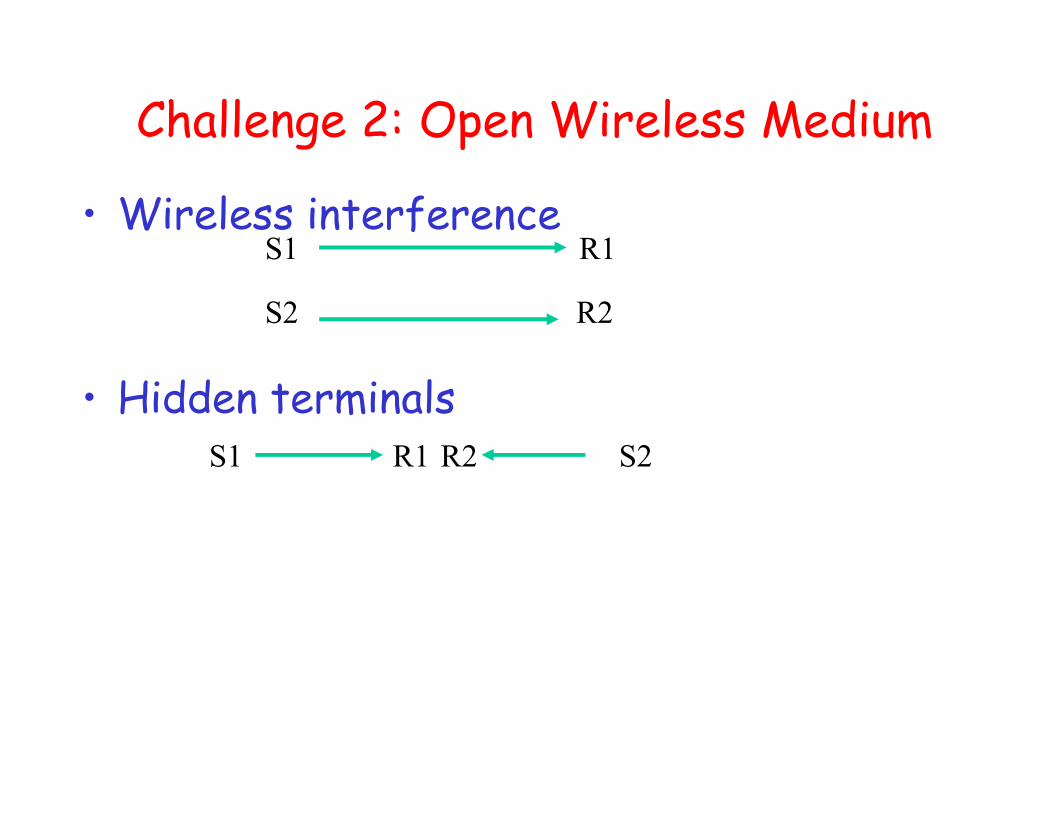
Challenge 2: Open Wireless Medium
• Wireless interference
S1
S2
R1
R2
Challenge 2: Open Wireless Medium
• Wireless interference
• Hidden terminals
S1
S2
R1
R2
S1 R1 S2R2
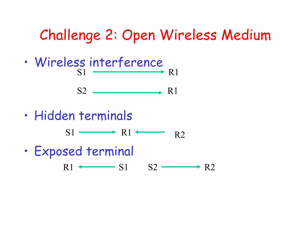
Challenge 2: Open Wireless Medium
• Wireless interference
• Hidden terminals
• Exposed terminal
S1
S2
R1
R1
S1 R1 R2
R1 S1 S2 R2

Challenge 2: Open Wireless Medium
• Wireless interference
• Hidden terminals
• Exposed terminal
• Wireless security– Eavesdropping, Denial of service, …
S1
S2
R1
R1
S1 R1 S2
R1 S1 S2 R2
Challenge 3: Intermittent Connectivity
• Reasons for intermittent connectivity– Mobility
– Environmental changes
• Existing networking protocols assume always-on networks
• Under intermittent connected networks– Routing, TCP, and applications all break
• Need a new paradigm to support communication under such environments
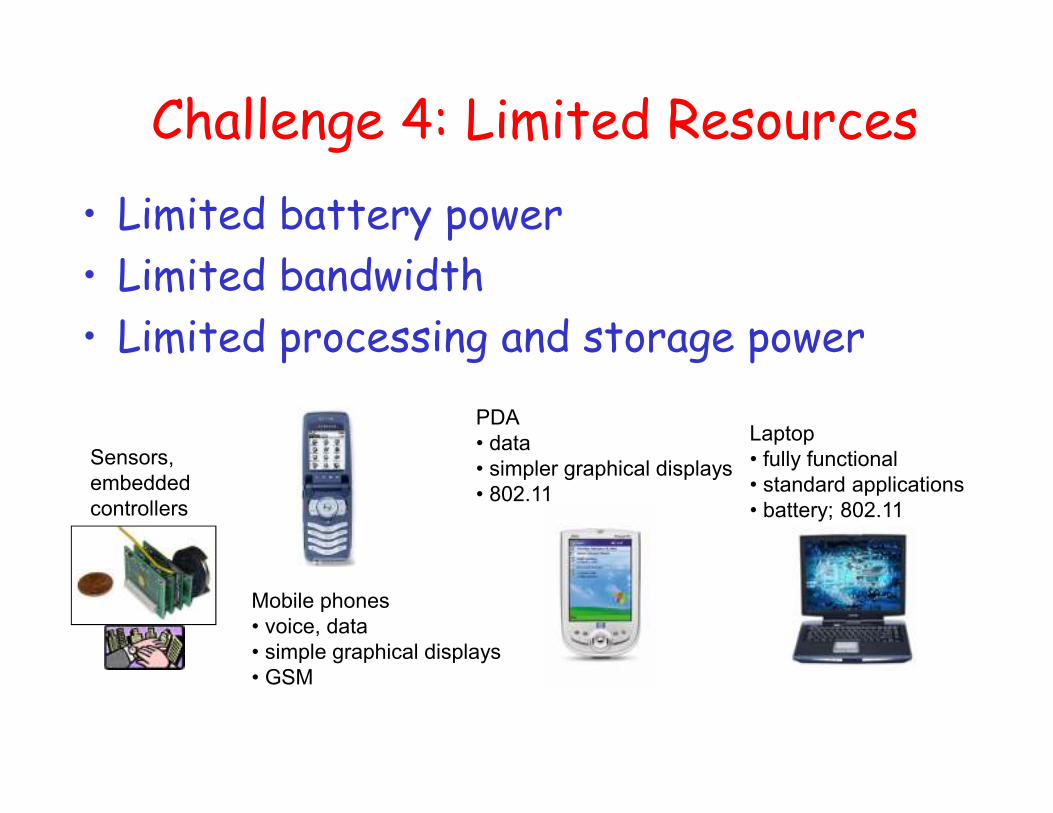
Challenge 4: Limited Resources
• Limited battery power
• Limited bandwidth
• Limited processing and storage power
Sensors,
embedded
controllers
Mobile phones
• voice, data
• simple graphical displays
• GSM
PDA
• data
• simpler graphical displays
• 802.11
Laptop
• fully functional
• standard applications
• battery; 802.11

Introduction to Wireless Networking

Internet Protocol Stack• Application: supporting network
applications– FTP, SMTP, HTTP
• Transport: data transfer between processes– TCP, UDP
• Network: routing of datagrams from source to destination– IP, routing protocols
• Link: data transfer between neighboring network elements– Ethernet, WiFi
• Physical: bits “on the wire”– Coaxial cable, optical fibers, radios
application
transport
network
link
physical

Physical Layer

Outline
• Signal
• Frequency allocation
• Signal propagation
• Multiplexing
• Modulation
• Spread Spectrum

Overview of Wireless Transmissions
source decoding
bit
streamchannel decoding
receiver
demodulation
source coding
bit
stream
channel coding
analog
signal
sender
modulation
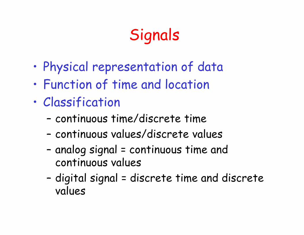
Signals
• Physical representation of data
• Function of time and location
• Classification– continuous time/discrete time
– continuous values/discrete values
– analog signal = continuous time and continuous values
– digital signal = discrete time and discrete values
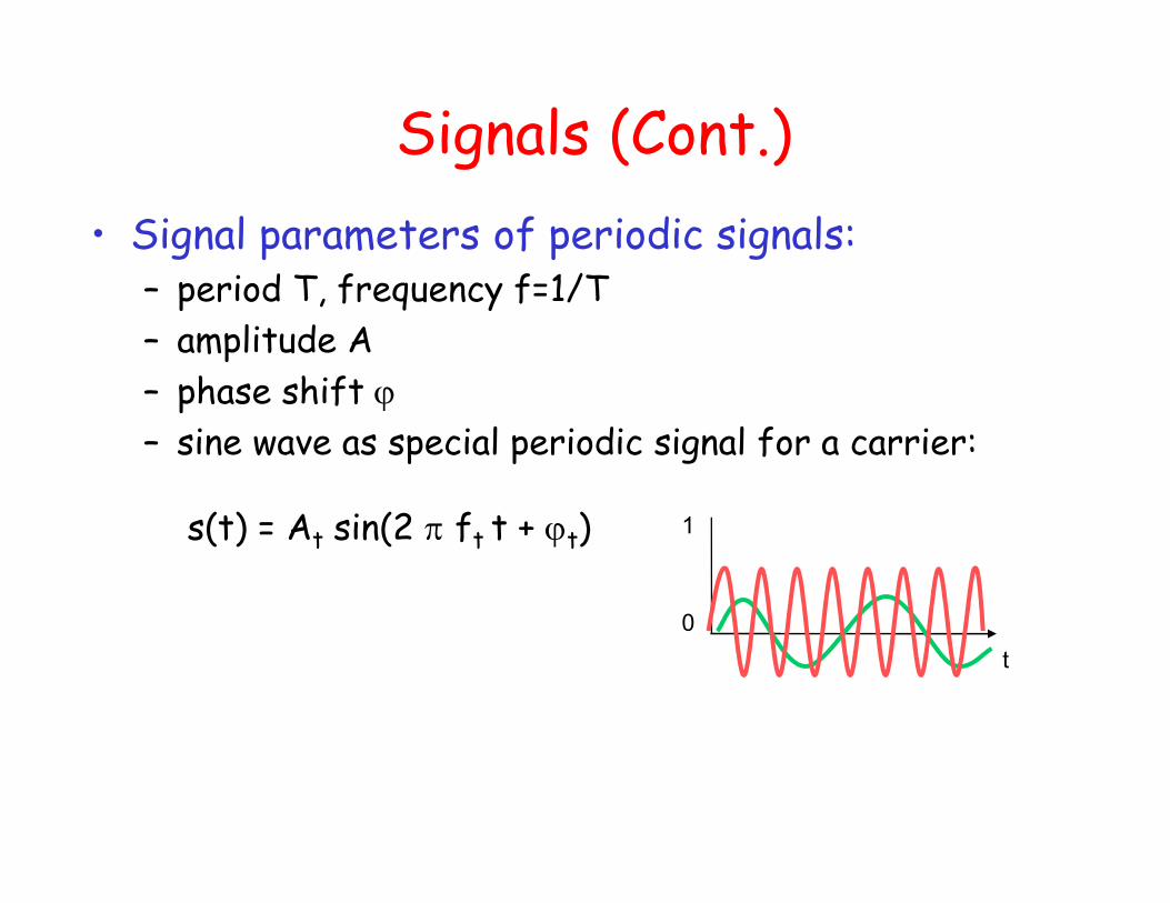
Signals (Cont.)
• Signal parameters of periodic signals: – period T, frequency f=1/T
– amplitude A
– phase shift ϕ
– sine wave as special periodic signal for a carrier:
s(t) = At sin(2 π ft t + ϕt) 1
0
t
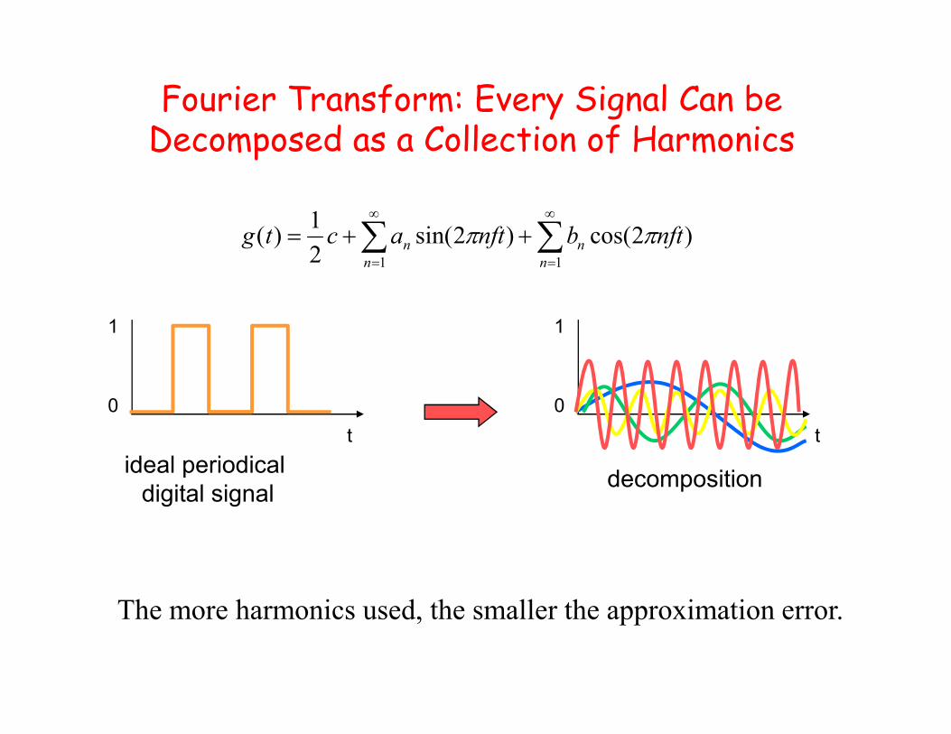
)2cos()2sin(2
1)(
11
nftbnftactgn
n
n
n ππ ∑∑∞
=
∞
=
++=
1
0
1
0
t t
ideal periodical
digital signaldecomposition
Fourier Transform: Every Signal Can be Decomposed as a Collection of Harmonics
The more harmonics used, the smaller the approximation error.

Why Not Send Digital Signal in Wireless Communications?
• Digital signals need– infinite frequencies for perfect transmission
– however, we have limited frequencies in wireless communications

Frequencies for Communication
VLF = Very Low Frequency UHF = Ultra High Frequency
LF = Low Freq., submarine SHF = Super High Frequency
MF = Medium Freq., radio EHF = Extra High Frequency
HF = High Freq., radio Visible light
VHF = Very High Frequency, TV UV = Ultraviolet Light
Frequency and wave length: λ = c/f , wave length λ, speed of light c ≅3x10⁸m/s, frequency f
1 Mm
300 Hz
10 km
30 kHz
100 m
3 MHz
1 m
300 MHz
10 mm
30 GHz
100 µm
3 THz
1 µm
300 THz
visible lightVLF LF MF HF VHF UHF SHF EHF infrared UV
optical transmissioncoax cabletwisted
pair
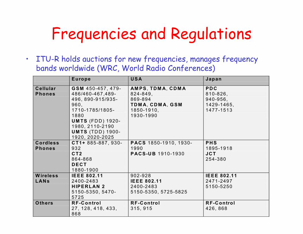
• ITU-R holds auctions for new frequencies, manages frequency bands worldwide (WRC, World Radio Conferences) Europe USA Japan
Cellular Phones
GSM 450-457, 479-486/460-467,489-496, 890-915/935-960, 1710-1785/1805-1880 UMTS (FD D) 1920-1980, 2110-2190 UMTS (TD D) 1900-1920, 2020-2025
AMPS , TDMA , CDMA 824-849, 869-894 TDMA , CDMA , GSM 1850-1910, 1930-1990
PDC 810-826, 940-956, 1429-1465, 1477-1513
Cordless Phones
CT1+ 885-887, 930-932 CT2 864-868 DECT 1880-1900
PACS 1850-1910, 1930-1990 PACS-UB 1910-1930
PHS 1895-1918 JCT 254-380
Wireless LANs
IEEE 802.11 2400-2483 HIPERLAN 2 5150-5350, 5470-5725
902-928 IEEE 802.11 2400-2483 5150-5350, 5725-5825
IEEE 802.11 2471-2497 5150-5250
Others RF-Control 27, 128, 418, 433, 868
RF-Control 315, 915
RF-Control 426, 868
Frequencies and Regulations
Why Need A Wide Spectrum
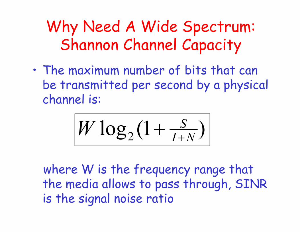
Why Need A Wide Spectrum: Shannon Channel Capacity
• The maximum number of bits that can be transmitted per second by a physical channel is:
where W is the frequency range that the media allows to pass through, SINR is the signal noise ratio
)1(log2 NISW ++
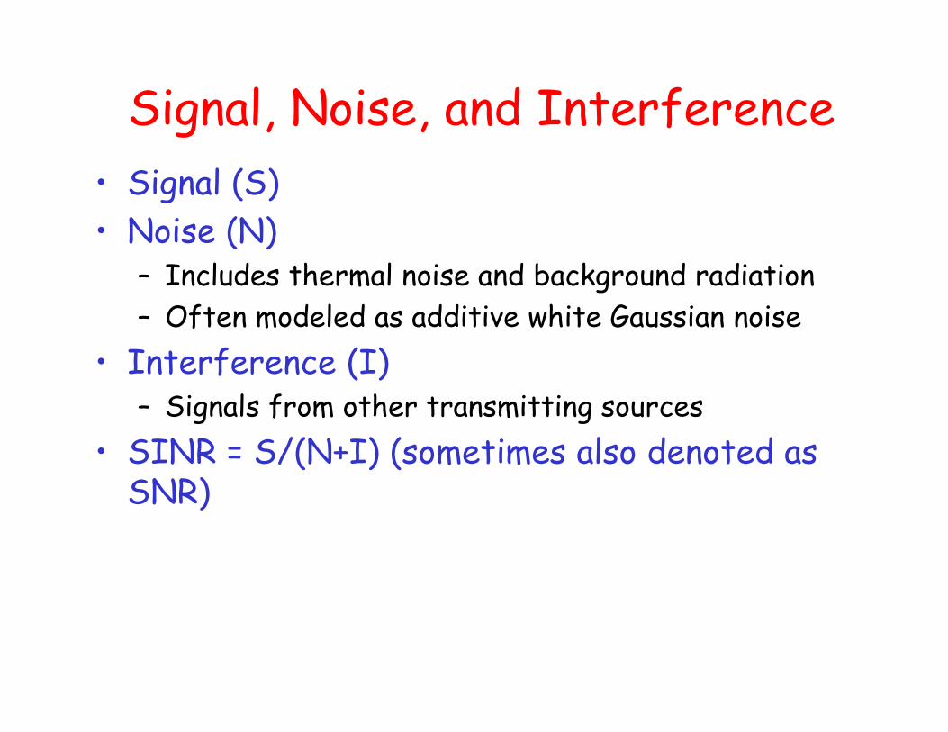
Signal, Noise, and Interference
• Signal (S)
• Noise (N)– Includes thermal noise and background radiation
– Often modeled as additive white Gaussian noise
• Interference (I)– Signals from other transmitting sources
• SINR = S/(N+I) (sometimes also denoted as SNR)

dB and Power conversion
• dB– Denote the difference between two power levels
– (P2/P1)[dB] = 10 * log10 (P2/P1)
– P2/P1 = 10^(A/10)
– Example: P2 = 100 P1 [Answer: 20dB], P2/P1=10 dB [Answer: P2/P1 = 10]
• dBm and dBW– Denote the power level relative to 1 mW or 1 W
– P[dBm] = 10*log10(P/1mW)
– P[dBW] = 10*log10(P/1W)
– Example: P = 0.001 mW [Answer: -30dBm], P = 100 W [Answer: 20dBW]

Outline
• Signal
• Frequency allocation
• Signal propagation
• Multiplexing
• Modulation
• Spread Spectrum
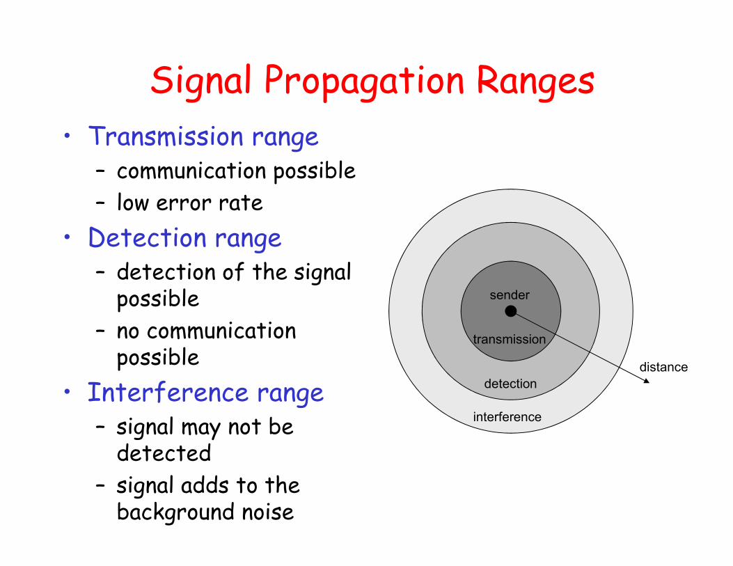
distance
sender
transmission
detection
interference
• Transmission range– communication possible
– low error rate
• Detection range– detection of the signal
possible
– no communication possible
• Interference range– signal may not be
detected
– signal adds to the background noise
Signal Propagation Ranges

• Does signal propagation via a straight line?
Signal Propagation
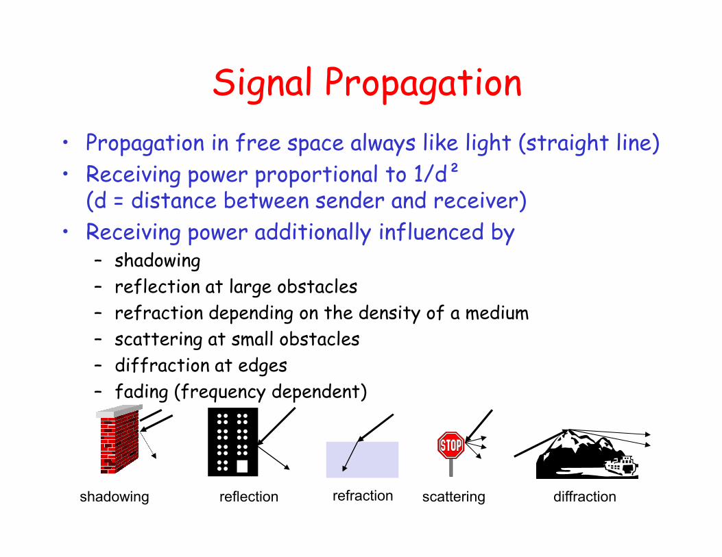
• Propagation in free space always like light (straight line)
• Receiving power proportional to 1/d² (d = distance between sender and receiver)
• Receiving power additionally influenced by– shadowing
– reflection at large obstacles
– refraction depending on the density of a medium
– scattering at small obstacles
– diffraction at edges
– fading (frequency dependent)
reflection scattering diffractionshadowing refraction
Signal Propagation

Path Loss
• Free space model
• Two-ray ground reflection model
• Log-normal shadowing
• Indoor model
• P = 1 mW at d0=1m, what’s Pr at d=2m?
Ld
GGPdP rtt
r 22
2
)4()(
πλ
=
Ld
hhGGPdP rtrtt
r 4
22
)( =
≥
<−−=
CnWWAFC
CnWWAFnW
d
dndBmdPdBmdP tr
*
*)log(10])[(])[(
0
σXdBdPdBdP += ])[(])[(
λπ /)4( rtc hhd =
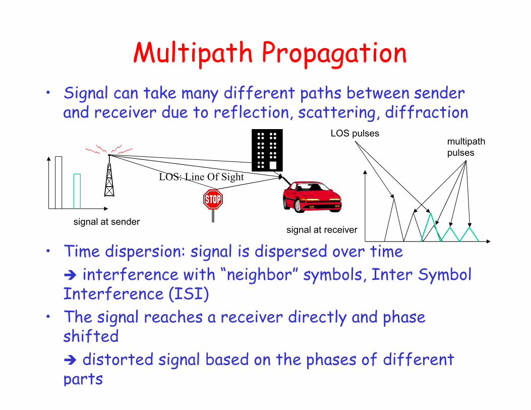
• Signal can take many different paths between sender and receiver due to reflection, scattering, diffraction
• Time dispersion: signal is dispersed over time
� interference with “neighbor” symbols, Inter Symbol Interference (ISI)
• The signal reaches a receiver directly and phase shifted
� distorted signal based on the phases of different parts
signal at sender
Multipath Propagation
signal at receiver
LOS pulsesmultipath
pulses
LOS: Line Of Sight

• Channel characteristics change over time and location – e.g., movement of sender, receiver and/or scatters
• � quick changes in the power received (short term/fast fading)
• Additional changes in– distance to sender
– obstacles further away
• � slow changes in the average power received (long term/slow fading)
short term fading
long term
fading
t
power
Fading

shadow fading
Rayleigh fading
path loss
log (distance)
Received
Signal
Power
(dB)
Typical Picture

Real world example

Outline
• Signal
• Frequency allocation
• Signal propagation
• Multiplexing
• Modulation
• Spread Spectrum
How to allow multiple nodes share the spectrum?

• Goal: multiple use of a shared medium
• Multiplexing in 4 dimensions– space (si)
– time (t)
– frequency (f)
– code (c)
• Important: guard spaces needed!
Multiplexing

Space Multiplexing
• Assign each region a channel
• Pros– no dynamic coordination
necessary
– works also for analog signals
• Cons– Inefficient resource
utilization
s2
s3
s1f
t
c
k2 k3 k4 k5 k6k1
f
t
c
f
t
c
channels ki

Frequency Multiplexing
• Separation of the whole spectrum into smaller frequency bands
• A channel gets a certain band of the spectrum for the whole time
• Pros:– no dynamic coordination
necessary
– works also for analog signals
• Cons:– waste of bandwidth
if the traffic is distributed unevenly
– Inflexible
– guard spaces
k2 k3 k4 k5 k6k1
f
t
c
f
t
c
k2 k3 k4 k5 k6k1
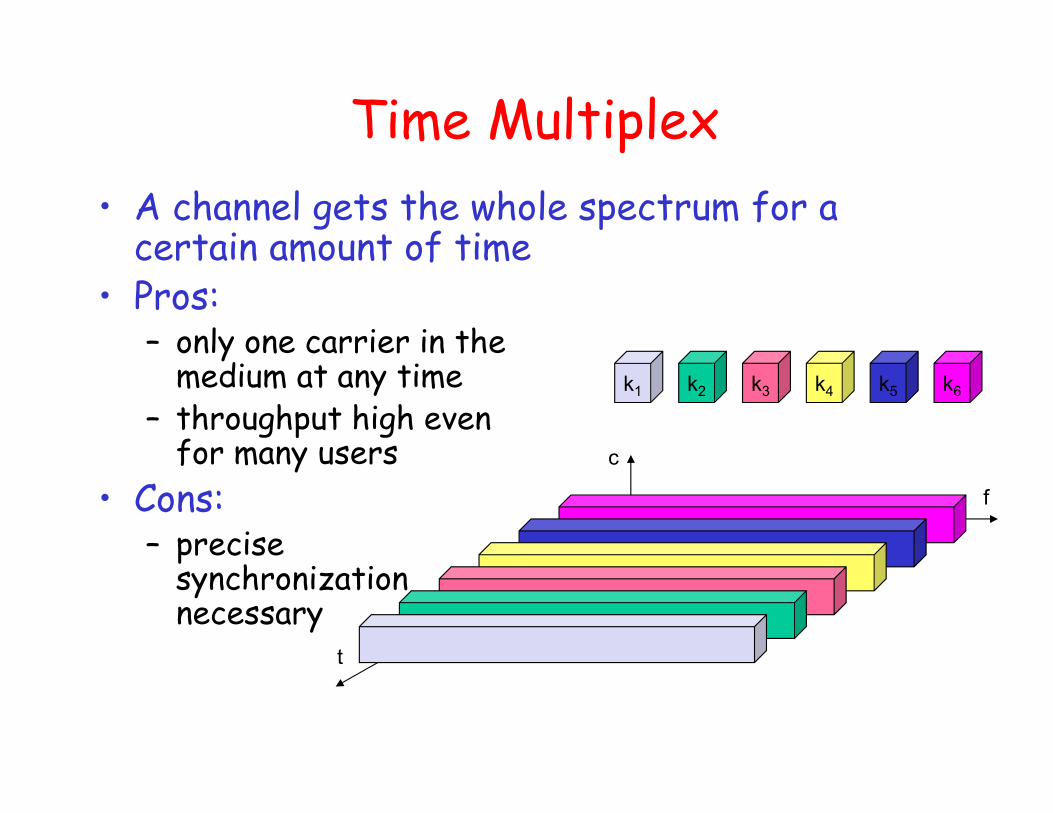
Time Multiplex
• A channel gets the whole spectrum for a certain amount of time
• Pros:– only one carrier in the
medium at any time– throughput high even
for many users
• Cons:– precise
synchronization necessary
f
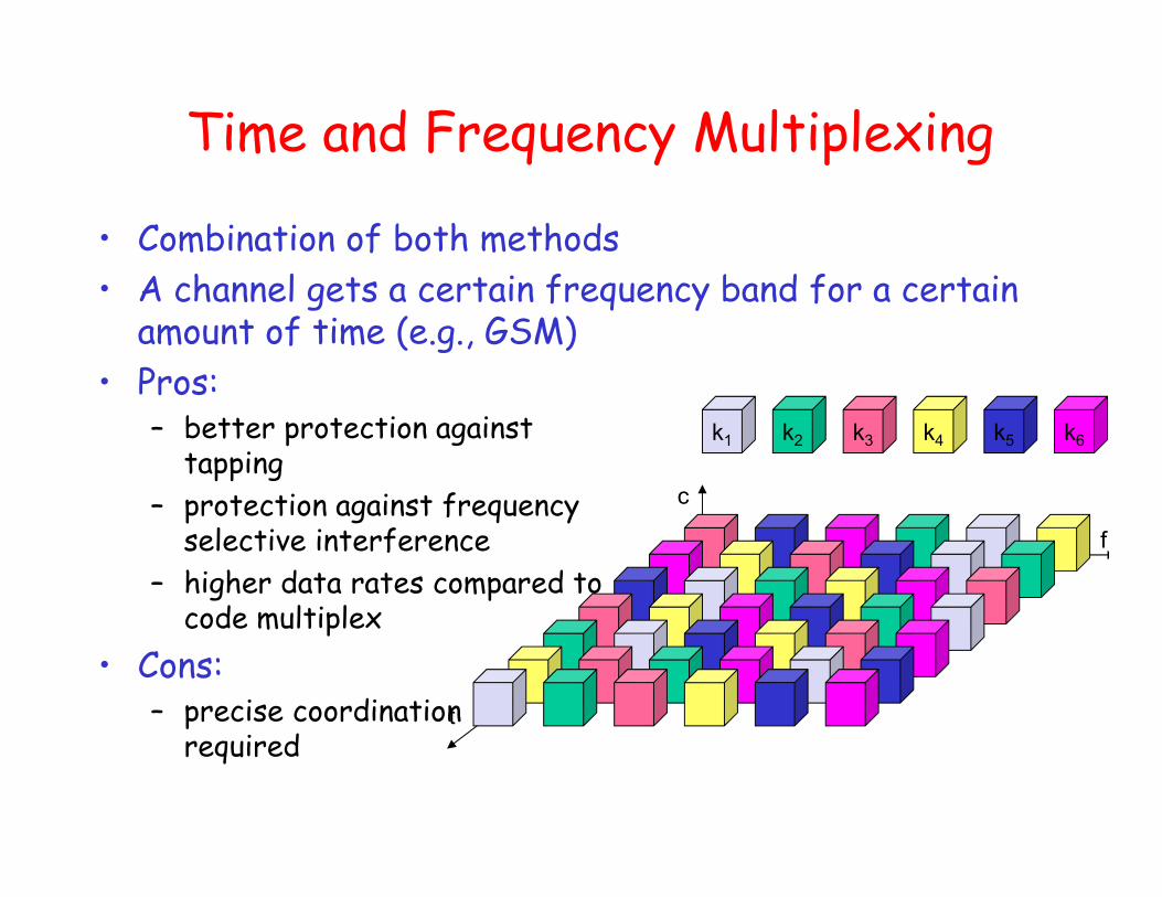
Time and Frequency Multiplexing
• Combination of both methods
• A channel gets a certain frequency band for a certain amount of time (e.g., GSM)
• Pros:– better protection against
tapping
– protection against frequency selective interference
– higher data rates compared tocode multiplex
• Cons:– precise coordination
requiredt
c
k2 k3 k4 k5 k6k1

Code Multiplexing• Each channel has a unique code
• All channels use the same spectrum simultaneously
• Pros:– bandwidth efficient
– no coordination and synchronization necessary
– good protection against interference and tapping
• Cons:– more complex signal regeneration
– need precise power control
• Implemented using spread spectrum technology
k2 k3 k4 k5 k6k1
f
t
c

Outline
• Signal
• Frequency allocation
• Signal propagation
• Multiplexing
• Modulation
• Spread Spectrum

Modulation I• Digital modulation
– Digital data is translated into an analog signal (baseband)
– Difference in spectral efficiency, power efficiency, robustness
• Analog modulation– Shifts center frequency of baseband signal up
to the radio carrier
– Reasons?

Modulation I• Digital modulation
– Digital data is translated into an analog signal (baseband)
– Difference in spectral efficiency, power efficiency, robustness
• Analog modulation– Shifts center frequency of baseband signal up
to the radio carrier
– Reasons• Antenna size is on the order of signal’s wavelength
• More bandwidth available at higher carrier frequency
• Medium characteristics: path loss, shadowing, reflection, scattering, diffraction depend on the signal’s wavelength

Modulation and Demodulation
digital
modulation
digital
data analog
modulation
radio
carrier
analog
baseband
signal
101101001 radio transmitter
synchronization
decision
digital
dataanalog
demodulation
radio
carrier
analog
baseband
signal
101101001 radio receiver

Modulation Schemes
• Amplitude Modulation (AM)
• Frequency Modulation (FM)
• Phase Modulation (PM)
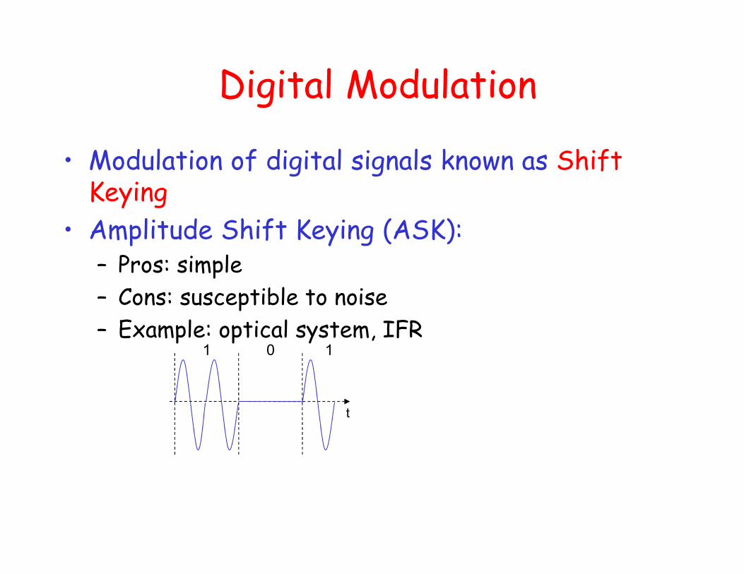
• Modulation of digital signals known as Shift Keying
• Amplitude Shift Keying (ASK):– Pros: simple
– Cons: susceptible to noise
– Example: optical system, IFR1 0 1
t
Digital Modulation

Digital Modulation II
• Frequency Shift Keying (FSK):– Pros: less susceptible to noise
– Cons: requires larger bandwidth
1 0 1
t
1 0 1
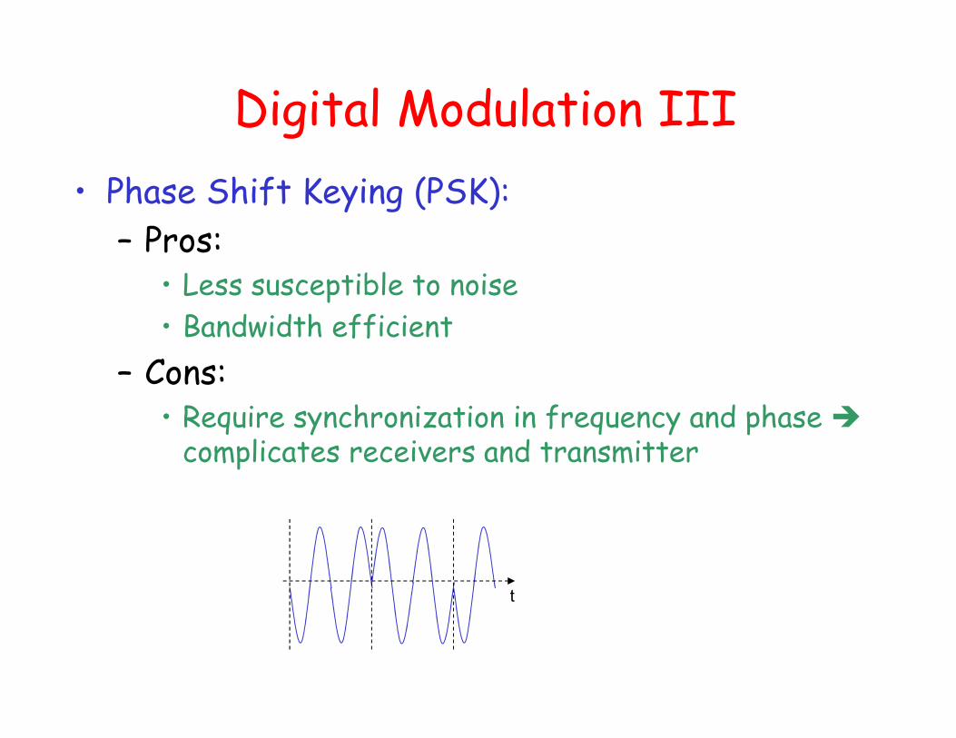
Digital Modulation III
• Phase Shift Keying (PSK):
– Pros: • Less susceptible to noise
• Bandwidth efficient
– Cons:• Require synchronization in frequency and phase �
complicates receivers and transmitter
t

• BPSK (Binary Phase Shift Keying):– bit value 0: sine wave
– bit value 1: inverted sine wave
– very simple PSK
– low spectral efficiency
– robust, used in satellite systems
Q
I01
Phase Shift Keying
11 10 00 01
Q
I
11
01
10
00
A
t
• QPSK (Quadrature Phase Shift Keying):– 2 bits coded as one symbol
– needs less bandwidth compared to BPSK
– symbol determines shift of sine wave
– Often also transmission of relative, not absolute phase shift: DQPSK -Differential QPSK
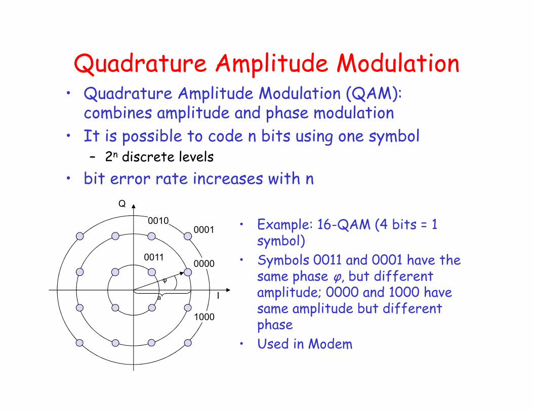
• Quadrature Amplitude Modulation (QAM): combines amplitude and phase modulation
• It is possible to code n bits using one symbol– 2n discrete levels
• bit error rate increases with n
0000
0001
0011
1000
Q
I
0010
φ
a
Quadrature Amplitude Modulation
• Example: 16-QAM (4 bits = 1 symbol)
• Symbols 0011 and 0001 have the same phase φ, but different amplitude; 0000 and 1000 have same amplitude but different phase
• Used in Modem
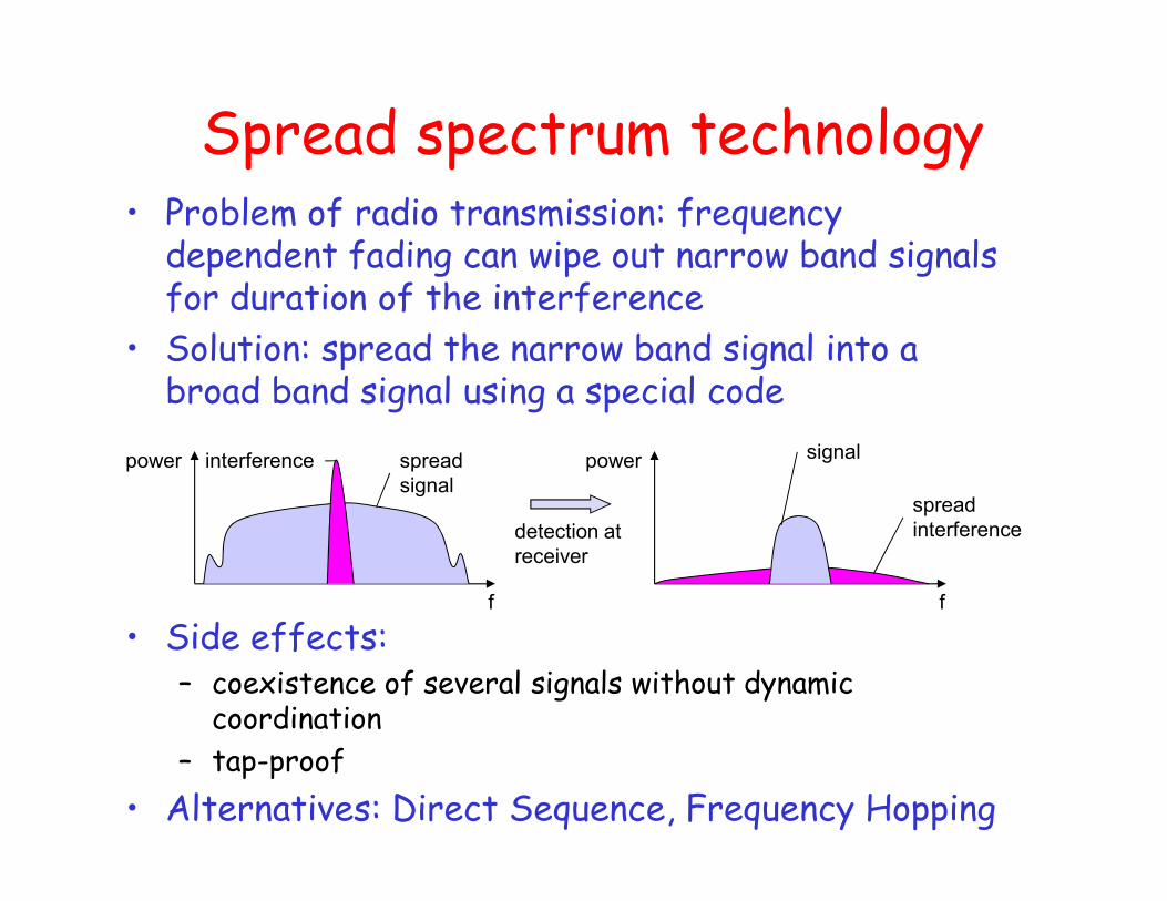
Spread spectrum technology• Problem of radio transmission: frequency
dependent fading can wipe out narrow band signals for duration of the interference
• Solution: spread the narrow band signal into a broad band signal using a special code
• Side effects:– coexistence of several signals without dynamic
coordination
– tap-proof
• Alternatives: Direct Sequence, Frequency Hopping
detection at
receiver
interference spread
signal
signal
spread
interference
f f
power power
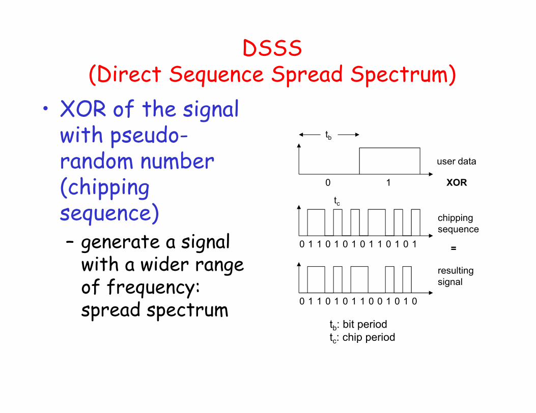
DSSS (Direct Sequence Spread Spectrum)
• XOR of the signal with pseudo-random number (chipping sequence)– generate a signal
with a wider range of frequency: spread spectrum
user data
chipping
sequence
resulting
signal
0 1
0 1 1 0 1 0 1 01 0 0 1 11
XOR
0 1 1 0 0 1 0 11 0 1 0 01
=
tb
tc
tb: bit period
tc: chip period
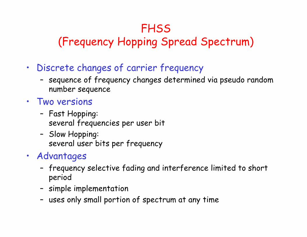
• Discrete changes of carrier frequency– sequence of frequency changes determined via pseudo random
number sequence
• Two versions– Fast Hopping:
several frequencies per user bit
– Slow Hopping: several user bits per frequency
• Advantages– frequency selective fading and interference limited to short
period
– simple implementation
– uses only small portion of spectrum at any time
FHSS (Frequency Hopping Spread Spectrum)

FHSS: Example
user data
slow
hopping
(3 bits/hop)
fast
hopping
(3 hops/bit)
0 1
tb
0 1 1 t
f
f1
f2
f3
t
td
f
f1
f2
f3
t
td
tb: bit period td: dwell time
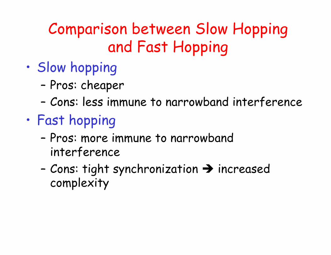
Comparison between Slow Hopping and Fast Hopping
• Slow hopping– Pros: cheaper
– Cons: less immune to narrowband interference
• Fast hopping– Pros: more immune to narrowband
interference
– Cons: tight synchronization � increased complexity


