CS262 Lecture Notes: Hidden Markov Models Sarah S January 21 2016 1 Summary Last lecture introduced hidden Markov models, and began to discuss some of the algorithms that can be used with HMMs to learn about sequences. In this lecture, we dive more deeply into the capabilities of HMMs, focusing mostly on their use in evaluation. We discuss higher order HMMs, and end with a brief discussion of HMM learning, to be expanded on in the next lecture. 2 CpG Islands The main example used to illustrate the concepts of HMMs is the idea of “CpG islands.” The notation ‘CpG’ indicates two adjacent nucleotides, a C and a G (these are next to each other, not paired across the strand — the p stands for the phosphate inbetween the cytosine and guanine). CpG islands are inter- esting because the distribution of adjacent Cs and Gs is different from other nucleotide pairs — they occur much less often than you’d expect in the overall genome (“CG supression”). However, there are places in the genome where they occur much more often. These are CpG islands, and they’re interesting because they tend to be methy- lated (an extra methyl is added to a cytosine base). Methylation closes up the structure of the strand, making it too close together for the transcription enzymes to get to — so the section can’t be transcribed. When this happens near a promoter, and entire gene can be permanently silenced. Over 60% of promoters occur in CpG islands. 1
Transcript
CS262 Lecture Notes: Hidden Markov Models
Sarah S
January 21 2016
1 Summary
Last lecture introduced hidden Markov models, and began to discuss some ofthe algorithms that can be used with HMMs to learn about sequences. In thislecture, we dive more deeply into the capabilities of HMMs, focusing mostly ontheir use in evaluation. We discuss higher order HMMs, and end with a briefdiscussion of HMM learning, to be expanded on in the next lecture.
2 CpG Islands
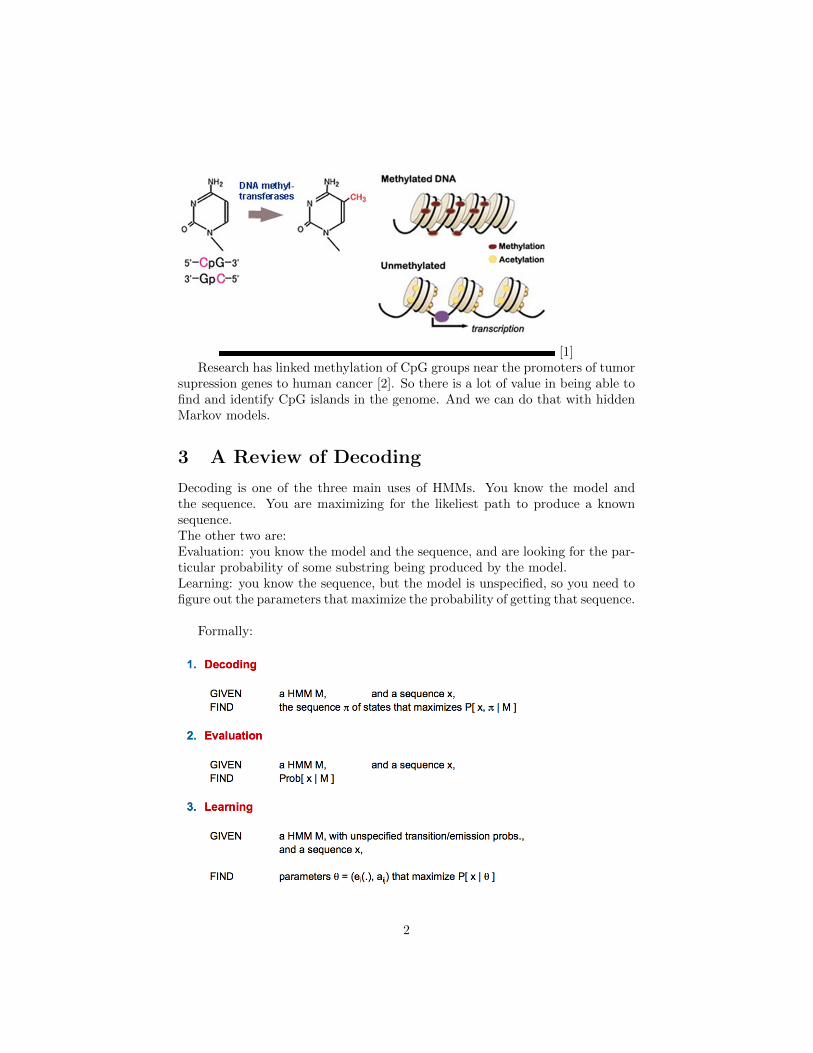
The main example used to illustrate the concepts of HMMs is the idea of “CpGislands.” The notation ‘CpG’ indicates two adjacent nucleotides, a C and a G(these are next to each other, not paired across the strand — the p stands forthe phosphate inbetween the cytosine and guanine). CpG islands are inter-esting because the distribution of adjacent Cs and Gs is different from othernucleotide pairs — they occur much less often than you’d expect in the overallgenome (“CG supression”).However, there are places in the genome where they occur much more often.These are CpG islands, and they’re interesting because they tend to be methy-lated (an extra methyl is added to a cytosine base). Methylation closes upthe structure of the strand, making it too close together for the transcriptionenzymes to get to — so the section can’t be transcribed. When this happensnear a promoter, and entire gene can be permanently silenced. Over 60% ofpromoters occur in CpG islands.
1
[1]Research has linked methylation of CpG groups near the promoters of tumor
supression genes to human cancer [2]. So there is a lot of value in being able tofind and identify CpG islands in the genome. And we can do that with hiddenMarkov models.
3 A Review of Decoding
Decoding is one of the three main uses of HMMs. You know the model andthe sequence. You are maximizing for the likeliest path to produce a knownsequence.The other two are:Evaluation: you know the model and the sequence, and are looking for the par-ticular probability of some substring being produced by the model.Learning: you know the sequence, but the model is unspecified, so you need tofigure out the parameters that maximize the probability of getting that sequence.
Formally:
2
Consider the question of decoding in the context of CpG islands. Decodingcan tell you which areas are islands, and which are not, by determining whatpath is most likely to have led to the sequence at hand. (For detailed formulasand math, see the notes from last lecture)
4 Evaluation
This determines the likelihood a sequence is generated by a particular model.Or, given the sequence and the model, what is the most likely state at someposition? If you remember the casino example (a casino is switching in a loadeddie that rolls sixes half the time), evaluation asks “is a particular region loadedor fair?” You pick a particular area, then compare against all possible states tofind out what the greatest probability is. (N.B. remember to account for theprobability cost of switching between states at the borders of the selected area.)Specifically, Evaluation can compute:P(x) – Probability of x given the modelP (xi. . . xj) – Probability of a substring of x given the modelP (πi = k|x) – “Posterior” probability that the ith state is k, given x
So how do you calculate P(x) given the model? With a “forward probability.”The forward probability is the probability that some position xi is what it is,given everything that came before. So, sum over all possible ways of generatingx: P (x) =
∑π P (x, π) =π P (x|π)P (π)
Seems reasonable, but this creates an exponential number of paths! Luckily,we don’t have to deal with all of them. Really all we care about is generatingthe first i characters of x, and ending up in state k. So we can simplify to:fk(i) = P (x1. . . xi, πi = k).
This leads to fk(i) = ek(xi)∑l fl(i–1)alk
Derivation:
fk(i) = P (x1...xi, πi = k)
use probability rules to obtain:
3
=∑π1...πi−1
P (x1...xi−1, π1....πi−1, πi = k)ek(xi)
ek(xi) is the emission probability, i.e. the probability that state k will emitthe value xi
=∑l
∑π1...πi−2
P (x1...xi−1, π1....πi−2, πi−1 = l)alkek(xi)alk is the transition probability, that between states πi−1 and πi we will
transition from state l to state k
Simplify:=
∑l P (x1...xi−1, πi−1 = l)alkek(xi)
And now using the original definition:= ek(xi)
∑l fl(i− 1)alk
Now that we know how to get a forward probability, how do we figure outthe maximum probability? Dynamic programming!Initialization: f0(0) = 1 and fk(0) = 0, for all k ¿ 0Iteration: fk(i) = ek(xi)
∑l fl(i–1)alk
Termination: P (x) =∑k fk(N)
7 Backwards Algorithm
Now, what if we want some P (πi = k|x), the probability distribution that theith position is k, given x? We need a helper to figure out the probability at ourpoint of interest. We already have the forward probability — now we need thebackwards probability.Fun fact! P(x) can be defined with the backwards probability as well as theforward —- they are identical in their structure of computational steps andrecursion.
7.1 Derivation of backwards probability
Define the backward probability: Starting from ith state = k, generate rest of xbk(i) = P (xi + 1. . . xN |πi = k)
And again, dynamic programming saves the day, as we find the best proba-bility by computing bk(i) for all k, i
Initialization: bk(N) = 1, for all k
Iteration: bk(i) =∑l el(xi+1)aklbl(i+ 1)
Termination: P (x) =∑l a0lel(x1)bl(1)
7.2 Computational Complexity for forward and backward
Not great. O(K2N) time, and O(KN) space.
There’s also a danger of underflows, since all this multiplying decimals leadsto really small numbers. Remember that when using Viterbi, you can use thesum of logs to avoid underflow? Well, when computing Forward or Backwardprobabilities, you can rescale at each few positions by multiplying by a constant.That keeps the numbers big enough for the computer to handle.
8 Posterior Decoding:
Posterior probability asks: what is the most likely state at position i of sequencex? Or, what is the probability that the ith state is k, given x?
Since we’ve shown how to compute fk(i) and bk(i), we can calculate P (πi =k|x) = (fk(i)bk(i))/P (x)
Let’s introduce a bit of new notation:π̂i = argmaxkP (πi = k|x)
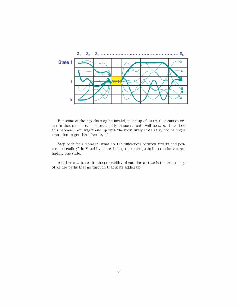
Posterior decoding produces a curve of likelihood of state for each position:
5
But some of these paths may be invalid, made up of states that cannot oc-cur in that sequence. The probability of such a path will be zero. How doesthis happen? You might end up with the most likely state at xi not having atransition to get there from xi−1!
Step back for a moment: what are the differences between Viterbi and pos-terior decoding? In Viterbi you are finding the entire path; in posterior you arefinding one state.
Another way to see it: the probability of entering a state is the probabilityof all the paths that go through that state added up.
6
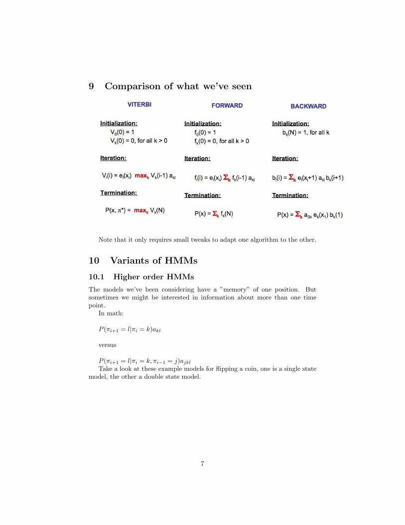
9 Comparison of what we’ve seen
Note that it only requires small tweaks to adapt one algorithm to the other.
10 Variants of HMMs
10.1 Higher order HMMs
The models we’ve been considering have a ”memory” of one position. Butsometimes we might be interested in information about more than one timepoint.
In math:
P (πi+1 = l|πi = k)akl
versus
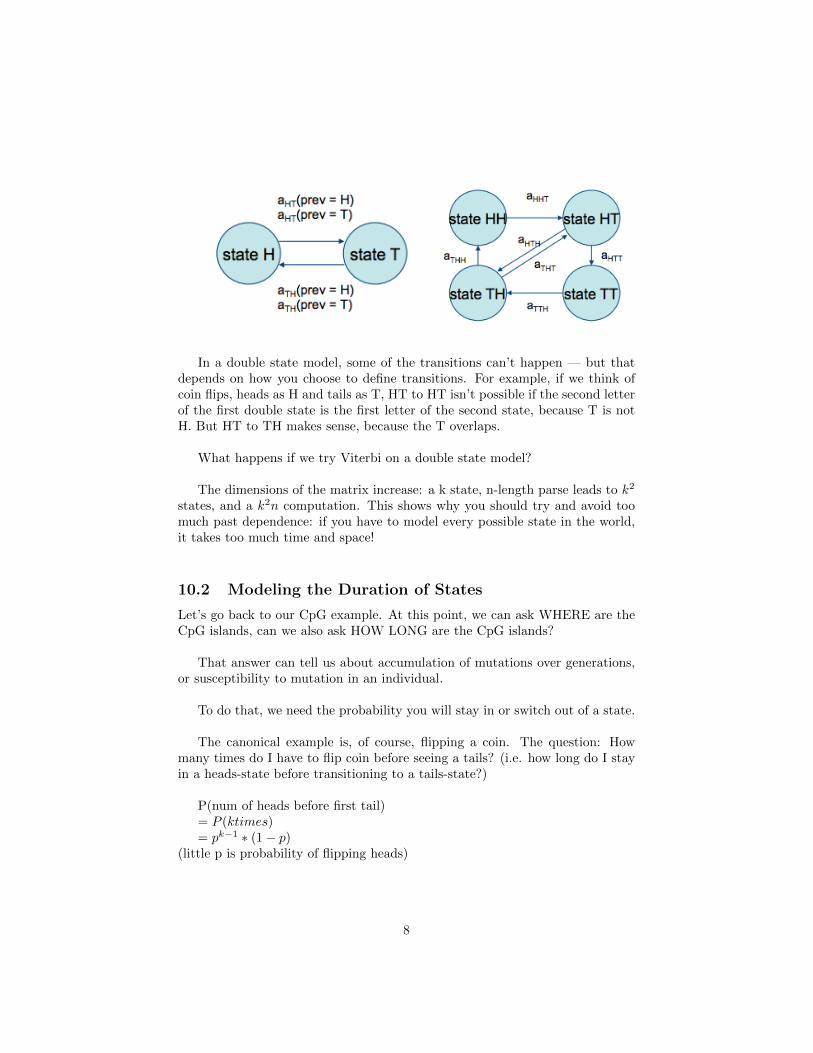
P (πi+1 = l|πi = k, πi−1 = j)ajklTake a look at these example models for flipping a coin, one is a single state
model, the other a double state model.
7
In a double state model, some of the transitions can’t happen — but thatdepends on how you choose to define transitions. For example, if we think ofcoin flips, heads as H and tails as T, HT to HT isn’t possible if the second letterof the first double state is the first letter of the second state, because T is notH. But HT to TH makes sense, because the T overlaps.
What happens if we try Viterbi on a double state model?
The dimensions of the matrix increase: a k state, n-length parse leads to k2
states, and a k2n computation. This shows why you should try and avoid toomuch past dependence: if you have to model every possible state in the world,it takes too much time and space!
10.2 Modeling the Duration of States
Let’s go back to our CpG example. At this point, we can ask WHERE are theCpG islands, can we also ask HOW LONG are the CpG islands?
That answer can tell us about accumulation of mutations over generations,or susceptibility to mutation in an individual.
To do that, we need the probability you will stay in or switch out of a state.
The canonical example is, of course, flipping a coin. The question: Howmany times do I have to flip coin before seeing a tails? (i.e. how long do I stayin a heads-state before transitioning to a tails-state?)
P(num of heads before first tail)= P (ktimes)= pk−1 ∗ (1− p)
(little p is probability of flipping heads)
8
Expectation[k] = 1/(1-p)Note that if p is large, 1-p is small, so E[k] is large.
This results in a geometric distribution.
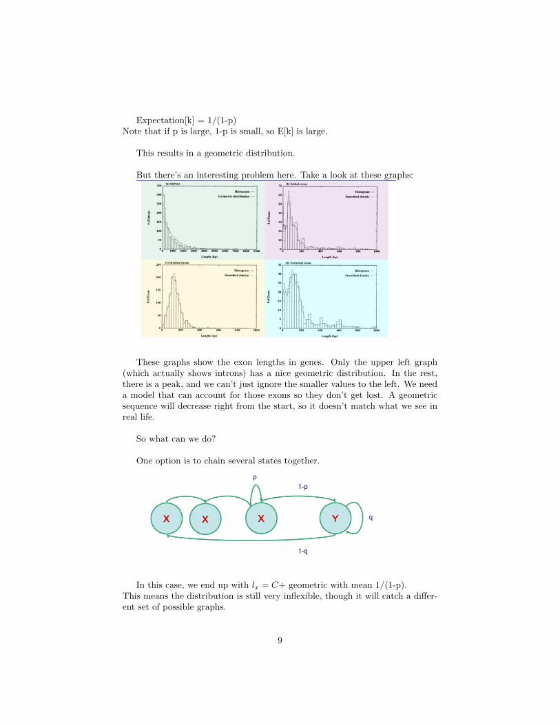
But there’s an interesting problem here. Take a look at these graphs:
These graphs show the exon lengths in genes. Only the upper left graph(which actually shows introns) has a nice geometric distribution. In the rest,there is a peak, and we can’t just ignore the smaller values to the left. We needa model that can account for those exons so they don’t get lost. A geometricsequence will decrease right from the start, so it doesn’t match what we see inreal life.
So what can we do?
One option is to chain several states together.
In this case, we end up with lx = C+ geometric with mean 1/(1-p).This means the distribution is still very inflexible, though it will catch a differ-ent set of possible graphs.
9
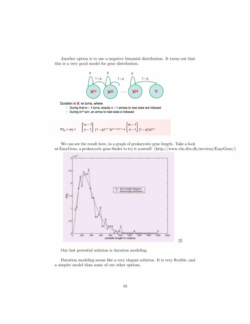
Another option is to use a negative binomial distribution. It turns out thatthis is a very good model for gene distribution.
We can see the result here, in a graph of prokaryotic gene length. Take a lookat EasyGene, a prokaryotic gene-finder to try it yourself. (http://www.cbs.dtu.dk/services/EasyGene/)
[3]
Our last potential solution is duration modeling.
Duration modeling seems like a very elegant solution. It is very flexible, anda simpler model than some of our other options.
10
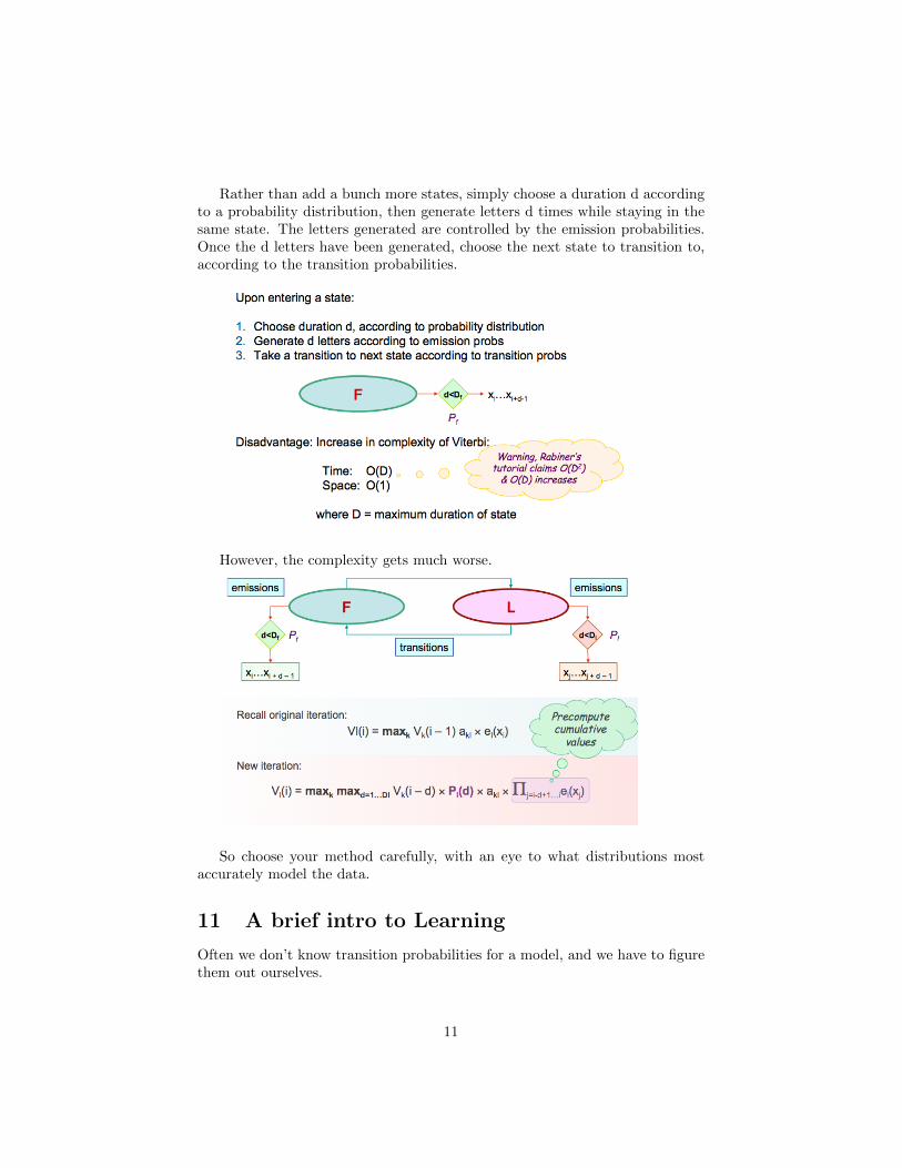
Rather than add a bunch more states, simply choose a duration d accordingto a probability distribution, then generate letters d times while staying in thesame state. The letters generated are controlled by the emission probabilities.Once the d letters have been generated, choose the next state to transition to,according to the transition probabilities.
However, the complexity gets much worse.
So choose your method carefully, with an eye to what distributions mostaccurately model the data.
11 A brief intro to Learning
Often we don’t know transition probabilities for a model, and we have to figurethem out ourselves.
11
Questions that can arise in that situation include:What is the distribution of a fair vs loaded die?What does a CpG island look like?
To answer these, we’ll recursively update paramaters to maximize P, usingexpectation maximization.
The biggest problem is overfitting to small data. Imagine if in your datasome output doesn’t show up – it will have a probability of zero in the cal-culated transition probabilities, if we’re simply counting how often we see anoutput in our data. But that might not be true!
Psuedocounts can compensate for overfitting. To guess a pseudo count, youcan use your prior beliefs or knowledge about a situation, or simply use verysmall probabilities to stand in for ones you don’t know anything about.
For a full treatment of this topic, see the next lecture.———
[2] See this 1983 Nature article for interesting early work in this area: ”Hy-pomethylation distinguishes genes of some human cancers from their normalcounterparts” – http://www.ncbi.nlm.nih.gov/pubmed/6185846