57
Behavioral Data Mining Lecture 12 Machine Biology

Behavioral Data Mining
Lecture 12
Machine Biology

Outline
• CPU geography
• Mass storage
• Buses and Networks
• Main memory
• Design Principles

Intel i7 close-up
From Computer Architecture a Quantitative Approach by Hennessy and Patterson,
as are most of the figures in this lecture.

Intel i7 close-up
From Computer Architecture a Quantitative Approach by Hennessy and Patterson

Intel i7 execution units
From Computer Architecture a Quantitative Approach by Hennessy and Patterson

Intel i7 caches
From Computer Architecture a Quantitative Approach by Hennessy and Patterson

i7 caches + memory management
From Computer Architecture a Quantitative Approach by Hennessy and Patterson

Motivation
We are going to focus on memory hierarchy in this lecture.
There are orders-of-magnitude differences between memory
speeds between different components and in different modes.
With behavioral data mining we have a lot of data to move into
and out of the processor, most of it in sparse matrices.
Memory (and cache) performance tend to dominate. There are
some important exceptions:
• Dense matrix operations, e.g. exact linear regression, factor
analysis, advanced gradient methods.
• Transcendental functions, exp, log, psi, etc
• Random number generation
Motivation
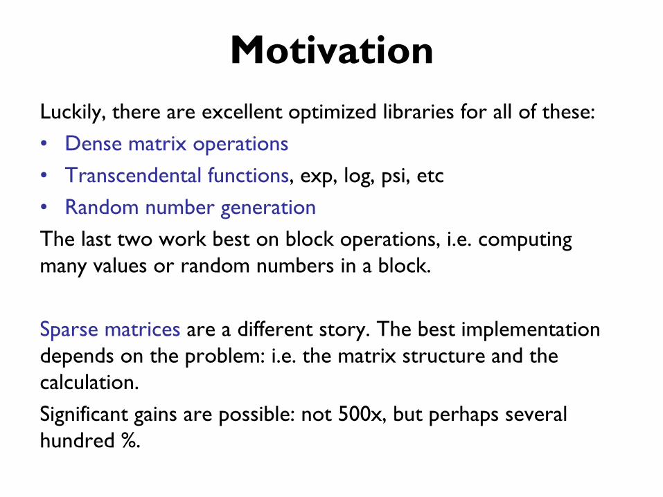
Luckily, there are excellent optimized libraries for all of these:
• Dense matrix operations
• Transcendental functions, exp, log, psi, etc
• Random number generation
The last two work best on block operations, i.e. computing
many values or random numbers in a block.
Sparse matrices are a different story. The best implementation
depends on the problem: i.e. the matrix structure and the
calculation.
Significant gains are possible: not 500x, but perhaps several
hundred %.

Memory Speeds
3x 3x 3x 5x 105
The speed range is huge (107) but most of it is memory-vs-disk
Note that these are random access times, not block access times.
Remarkably, dense matrix multiply runs at 100 Gflops: 1 flop
every 10ps ! That implies that each value must be processed many
times in inner cache, with processor parallelism fully exercised.
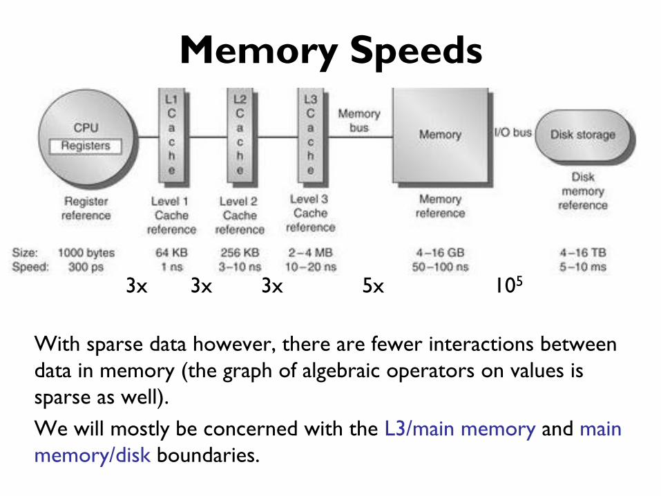
Memory Speeds
3x 3x 3x 5x 105
With sparse data however, there are fewer interactions between
data in memory (the graph of algebraic operators on values is
sparse as well).
We will mostly be concerned with the L3/main memory and main
memory/disk boundaries.
Outline
• CPU geography
• Mass storage
• Buses and Networks
• Main memory
• Design Principles
SSDs vs HDD
Flash-based solid-state drives open up new opportunities for fast
data mining – random access times are significantly faster.
Both HDD and SSD have similar read performance, currently
maxing out at the SATA bus rate of 6Gb/s.
Writing isn’t necessarily faster however.
Many ML algorithms (those based on gradient optimization or
MCMC) access training data sequentially.
Others make random accesses to data:
– Simplex
– Interior point methods (for linear and semi-definite
programming)
But have been eclipsed by SGD in many cases.

SSDs vs HDD

Maximizing Throughput
To maximize throughput for streaming operations, we can use
multiple disks, with or without RAID.
RAID-0 – no redundancy, just striping.
RAID-1 – simple mirroring –
Hadoop does this
Images from http://en.wikipedia.org/wiki/RAID
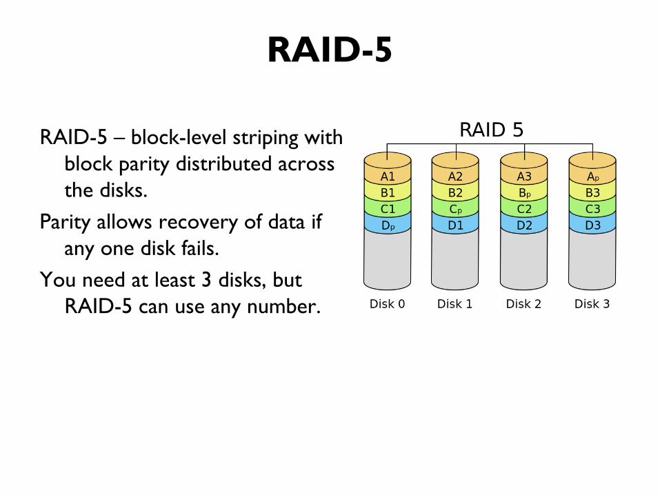
RAID-5
RAID-5 – block-level striping with
block parity distributed across
the disks.
Parity allows recovery of data if
any one disk fails.
You need at least 3 disks, but
RAID-5 can use any number.
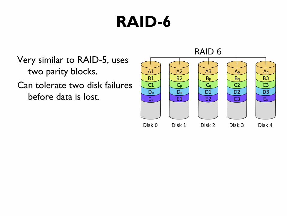
RAID-6
Very similar to RAID-5, uses
two parity blocks.
Can tolerate two disk failures
before data is lost.

JBOD
JBOD is “Just a Bunch Of Disks”
No coordination of data read-write:
Assumed that data is coarsely
partitioned.
Highest throughput: basically all
the disks run at full speed on
both read and write.
But the code must be multi-threaded to stream from each disk
independently.

Hybrids- e.g. Data Engine
You can use both software RAID and JBOD with the same disks
– assuming both modes are not normally used together.
16x individual disks (1TB partitions) – 100-200 MB/s R/W each
14 TB RAID-6, built from the other halves of the disks above.

RAID-6 speed
The software RAID-6 is about 10x the speed of one disk reading.

Outline
• CPU geography
• Mass storage
• Buses and Networks
• Main memory
• Design Principles

PCI Bus Evolution

Observations
• PCIe runs approximately at “memory speeds” rather than I/O
speeds (Most PCs ship with PCIe-3.0 at 16x or better)
• Recent benchmark:
– GPU transfer rate (w pinned memory) approximately the
same as CPU memory-to-memory (w/o pinning).
• Consequences:
– GPU-CPU transfers not a bottleneck anymore
– Given enough disks – you should in principle be able to
stream data at memory speeds (10s of GB/s).
– More realistically, do this with SSDs in a few years.
Network Evolution
Networks have evolved at similar rates, but we still have:
• Standard Ethernet: 1Gb/s and 10Gb/s
• Some high-end servers use Infiniband networking which can
run up to several 100 Gb/s.
• 100 Gb/s Ethernet exists (optical), but only in large network
backbones.
Demand for higher bandwidths seems very weak:
• Lack of high-speed data sources and sinks (disks can’t
normally handle higher rates)?
• Lack of algorithmic sources (synthetic data/animation)?

Network Topology
Switches provide contention-free, full rate communication
between siblings (normally machines in the same rack).
Communication between < 40 peers is usually significantly faster
than communication in a larger group.

Outline
• CPU geography
• Mass storage
• Buses and Networks
• Main memory
• Design Principles

Memory: Row/Column Access

Row vs Column Access

Burst Access
Cycle times limit how fast we can transfer data given a read
request in spite of the chip’s inner speed. But burst access
allows much higher speeds.

Burst Access
In burst mode, DRAM chips can stream e.g. 8 or more xfers in
response to a single memory request, giving these max rates
for transfers:

Random Access
Unfortunately, random access is actually getting worse:

Memory Banking
To increase bandwidth, DRAMs are divided into multiple
independent banks (usually 4). However, the mapping from
row, column, bank address is configurable (motherboard).
Most often(?) its interleaved (bank address is CPU address LSB)
Note, banking is RAM-card side, and independent of dual- or
triple-channel memory interfaces on the CPU.

Interleaved banks
Interleaving gives fastest possible speed for sequential access to a
single block of memory.
May not work as well for multiple blocks (copies), or in
particular for sparse matrix operations (like matrix-vector
multiply) that involve a single pass over the val, row arrays.
Documentation is poor for this spec – need to try some
benchmarks.
row
colptr
N
N
M+1
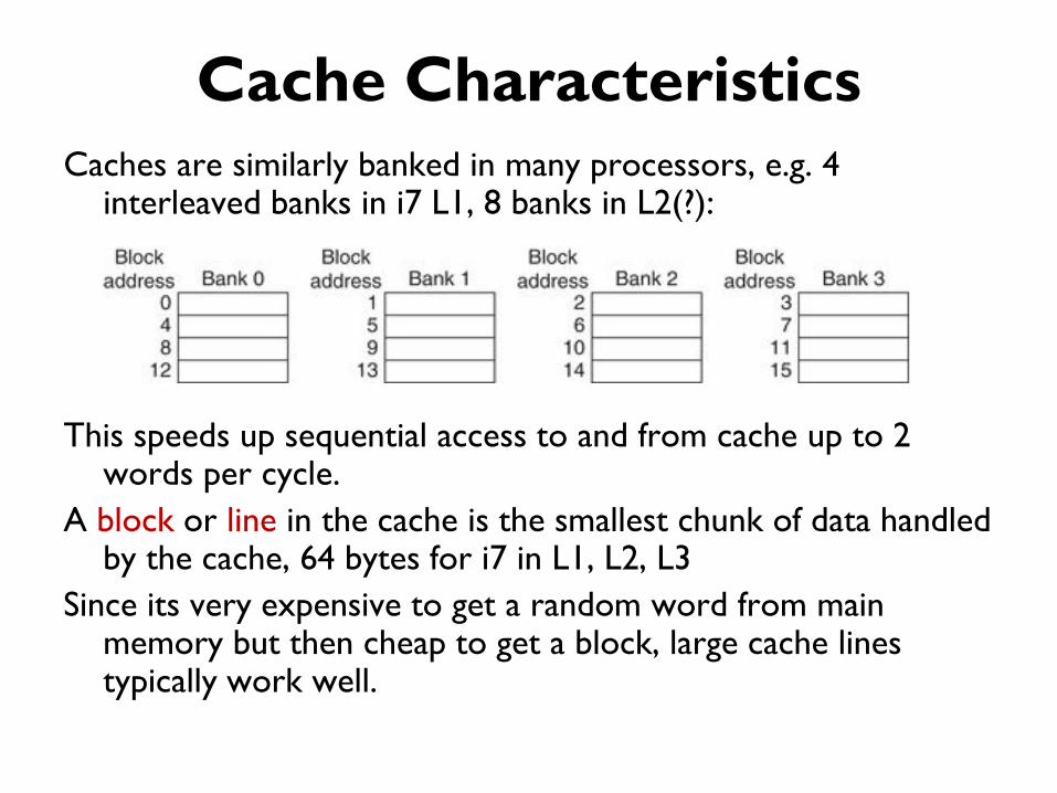
Cache Characteristics
Caches are similarly banked in many processors, e.g. 4 interleaved banks in i7 L1, 8 banks in L2(?):
This speeds up sequential access to and from cache up to 2 words per cycle.
A block or line in the cache is the smallest chunk of data handled by the cache, 64 bytes for i7 in L1, L2, L3
Since its very expensive to get a random word from main memory but then cheap to get a block, large cache lines typically work well.
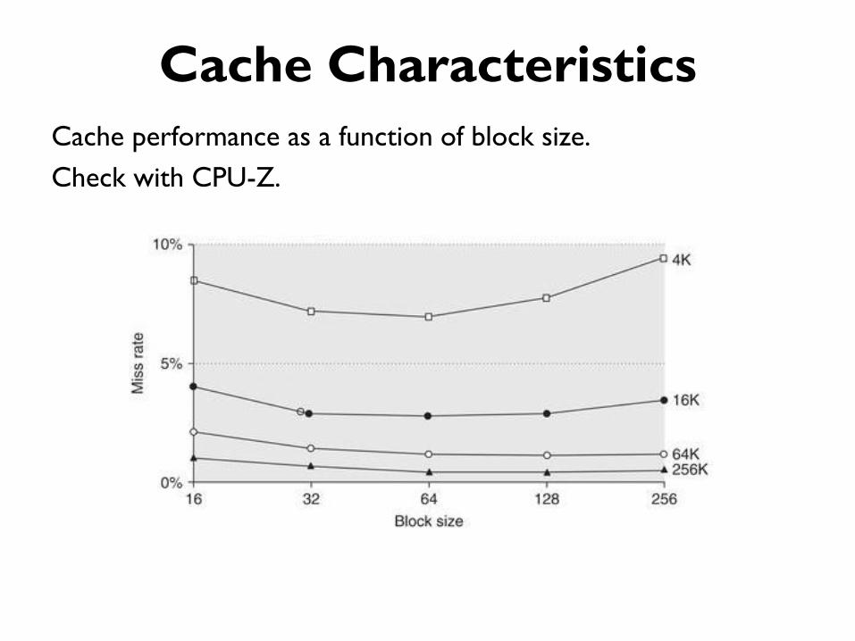
Cache Characteristics
Cache performance as a function of block size.
Check with CPU-Z.

Cache Mapping

CPU-Z
Y

CPU-Z
X
Y

CPU-Z
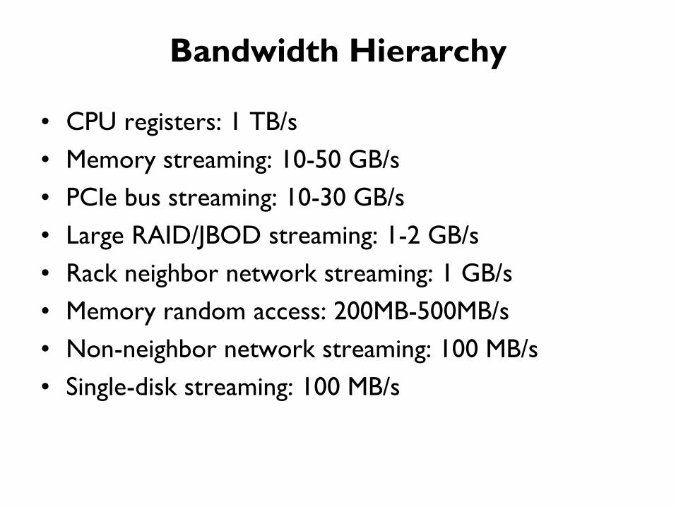
Bandwidth Hierarchy
• CPU registers: 1 TB/s
• Memory streaming: 10-50 GB/s
• PCIe bus streaming: 10-30 GB/s
• Large RAID/JBOD streaming: 1-2 GB/s
• Rack neighbor network streaming: 1 GB/s
• Memory random access: 200MB-500MB/s
• Non-neighbor network streaming: 100 MB/s
• Single-disk streaming: 100 MB/s

Outline
• CPU geography
• Mass storage
• Buses and Networks
• Main memory
• Design Principles
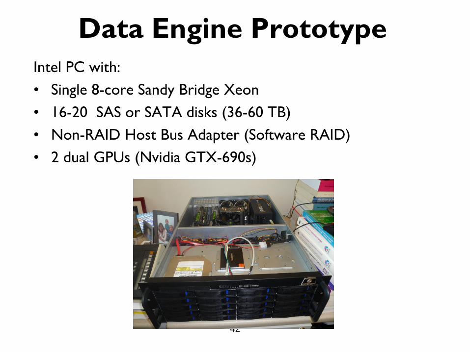
Data Engine Prototype
42
Intel PC with:
• Single 8-core Sandy Bridge Xeon
• 16-20 SAS or SATA disks (36-60 TB)
• Non-RAID Host Bus Adapter (Software RAID)
• 2 dual GPUs (Nvidia GTX-690s)

Optimizations
• Sort instead of hash: At least for large data sets:
– Sorting on one GPU is 2-4 GB/s
– Hashing on a CPU is 200-400 MB/s

Optimizations
• Merge arrays: several large arrays that are traversed together
(e.g. row, val arrays in sparse matrices) into one array of
alternating elements.
• Loop interchange: so array elements traversed in consecutive
order (lecture 1).
• Blocking: access array elements in blocks so both operands
and results stay in cache.

Cluster Issues
• In a Hadoop task however, the processor cores are working
on different data in different areas of memory.
• This is not a good match for interleaved banked memory –
unless the data spread out across memory chips.
• Future processors are including quad-port interfaces, which
isolate the cores memory accesses from each other.
46
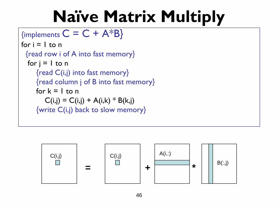
Naïve Matrix Multiply {implements C = C + A*B} for i = 1 to n
{read row i of A into fast memory}
for j = 1 to n
{read C(i,j) into fast memory}
{read column j of B into fast memory}
for k = 1 to n
C(i,j) = C(i,j) + A(i,k) * B(k,j)
{write C(i,j) back to slow memory}
= + *
C(i,j) A(i,:)
B(:,j)
C(i,j)

47
Blocked (Tiled) Matrix Multiply Consider A,B,C to be N-by-N matrices of b-by-b subblocks where
b=n / N is called the block size
for i = 1 to N
for j = 1 to N
{read block C(i,j) into fast memory}
for k = 1 to N
{read block A(i,k) into fast memory}
{read block B(k,j) into fast memory}
C(i,j) = C(i,j) + A(i,k) * B(k,j) {do a matrix multiply on blocks}
{write block C(i,j) back to slow memory}
= + *
C(i,j) C(i,j) A(i,k)
B(k,j)

Search Over Block Sizes • Performance models are useful for high level algorithms
– Helps in developing a blocked algorithm
– Models have not proven very useful for block size
selection
• too complicated to be useful
– See work by Sid Chatterjee for detailed model
• too simple to be accurate
– Multiple multidimensional arrays, virtual memory, etc.
– Speed depends on matrix dimensions, details of
code, compiler, processor
From CS267 SP11 notes

49
What the Search Space Looks Like
A 2-D slice of a 3-D register-tile search space. The dark blue region was pruned.
(Platform: Sun Ultra-IIi, 333 MHz, 667 Mflop/s peak, Sun cc v5.0 compiler)
Number of rows in register block

ATLAS (DGEMM n = 500)
• ATLAS is faster than all other portable BLAS implementations and it is comparable with machine-specific libraries provided by the vendor.
0.0
100.0
200.0
300.0
400.0
500.0
600.0
700.0
800.0
900.0
AM
D Ath
lon-
600
DEC
ev5
6-53
3
DEC
ev6
-500
HP90
00/7
35/1
35
IBM
PPC
604-
112
IBM
Pow
er2-
160
IBM
Pow
er3-
200
Pentiu
m P
ro-2
00
Pentiu
m II
-266
Pentiu
m II
I-550
SGI R
1000
0ip28
-200
SGI R
1200
0ip30
-270
Sun U
ltraS
parc2
-200
Architectures
MF
LO
PS
Vendor BLAS
ATLAS BLAS
F77 BLAS
Source: Jack Dongarra
From CS267 SP11 notes
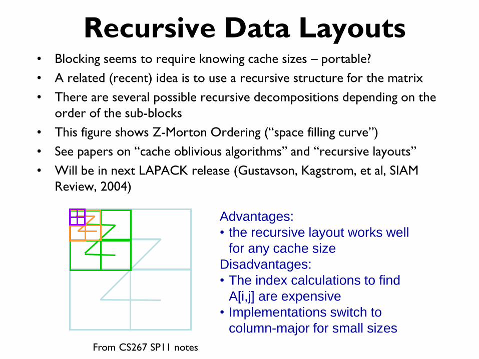
Recursive Data Layouts • Blocking seems to require knowing cache sizes – portable?
• A related (recent) idea is to use a recursive structure for the matrix
• There are several possible recursive decompositions depending on the
order of the sub-blocks
• This figure shows Z-Morton Ordering (“space filling curve”)
• See papers on “cache oblivious algorithms” and “recursive layouts”
• Will be in next LAPACK release (Gustavson, Kagstrom, et al, SIAM
Review, 2004)
Advantages:
• the recursive layout works well
for any cache size
Disadvantages:
• The index calculations to find
A[i,j] are expensive
• Implementations switch to
column-major for small sizes
From CS267 SP11 notes
Sparse Matrix-Vector Multiply
• The key step for many learning algorithms, especially gradient-
based methods. Sparse matrix = user data.
• There is similar work on automatic optimization of sparse
matrix algorithms.
• Examples:
– OSKI
– CSB (Compressed Sparse Blocks)

Summary of Performance Optimizations
• Optimizations for SpMV – Register blocking (RB): up to 4x over CSR
– Variable block splitting: 2.1x over CSR, 1.8x over RB
– Diagonals: 2x over CSR
– Reordering to create dense structure + splitting: 2x over CSR
– Symmetry: 2.8x over CSR, 2.6x over RB
– Cache blocking: 2.8x over CSR
– Multiple vectors (SpMM): 7x over CSR
– And combinations…
• Sparse triangular solve – Hybrid sparse/dense data structure: 1.8x over CSR
• Higher-level kernels – A·AT·x, AT·A·x: 4x over CSR, 1.8x over RB
– A2·x: 2x over CSR, 1.5x over RB
– [A·x, A2·x, A3·x, .. , Ak·x]

Optimized Sparse Kernel Interface
- OSKI
• Provides sparse kernels automatically tuned for user’s matrix & machine
– BLAS-style functionality: SpMV, Ax & ATy, TrSV
– Hides complexity of run-time tuning
– Includes new, faster locality-aware kernels: ATAx, Akx
• Faster than standard implementations
– Up to 4x faster matvec, 1.8x trisolve, 4x ATA*x
• For “advanced” users & solver library writers
– Available as stand-alone library (OSKI 1.0.1h, 6/07)
– Available as PETSc extension (OSKI-PETSc .1d, 3/06)
– Bebop.cs.berkeley.edu/oski
• Under development: pOSKI for multicore


Summary
• CPU geography
• Mass storage
• Buses and Networks
• Main memory
• Design Principles


