17
CS654: Digital Image Analysis Lecture 12: Separable Transforms
| Date post: | 31-Dec-2015 |
| Category: |
Documents |
| Upload: | jocelyn-taylor |
| View: | 220 times |
| Download: | 0 times |

CS654: Digital Image Analysis
Lecture 12: Separable Transforms
Recap of Lecture 11
• Image Transforms
• Source and target domain
• Unitary transform, 1-D
• Unitary transform, 2-D
• High computational complexity

Outline of Lecture 12
• Unitary transforms
• Separable functions
• Properties of unitary transforms

Image transforms
• Operation to change the default representation space of a digital image (source domain target domain)
• All the information present in the image is preserved in the transformed domain, but represented differently;
• The transform is reversible
• Source domain = spatial domain and target domain= frequency domain

Unitary transform
1}Nn0{u(n), 1-D input sequence
1N
0n1Nk0,n)u(n)a(k,v(k)ro,Auv
If Transformed sequence
1N
0k
*T* 1Nn0,n)v(k)(k,au(n)orvAu

2-D sequence
v(k,l) a (m,n) u(m,n) , 0 k,l N 1k,ln 0
N 1
m 0
N 1
=
[𝑎𝑘𝑙 (0 ,0 ) ⋯ 𝑎𝑘𝑙 (0 ,𝑛 ) ⋯ 𝑎𝑘𝑙 (0 ,𝑁−1 )
⋮ ⋯ ⋯ ⋯ ⋮𝑎𝑘𝑙 (𝑚 ,0 ) ⋯ 𝑎𝑘𝑙 (𝑚 ,𝑛) ⋯ 𝑎𝑘𝑙(𝑚 ,𝑁−1)
⋮ … … … ⋮𝑎𝑘𝑙(𝑁−1,0) … 𝑎𝑘𝑙(𝑁−1,𝑛) … 𝑎𝑘𝑙(𝑁−1 ,𝑁−1)
]×[
𝑢 (0 ,0 ) ⋯ 𝑢 (0 ,𝑛) ⋯ 𝑢 (0 ,𝑁−1 )⋮ ⋯ ⋯ ⋯ ⋮
𝑢 (𝑚 ,0 ) ⋯ 𝑢(𝑚 ,𝑛) … 𝑢 (𝑚 ,𝑁−1)⋮ … … … ⋮
𝑢(𝑁−1,0) … 𝑢(𝑁−1 ,𝑙) … 𝑢(𝑁−1 ,𝑁−1)]
High computational complexity
O(N4)
Separable Transformations
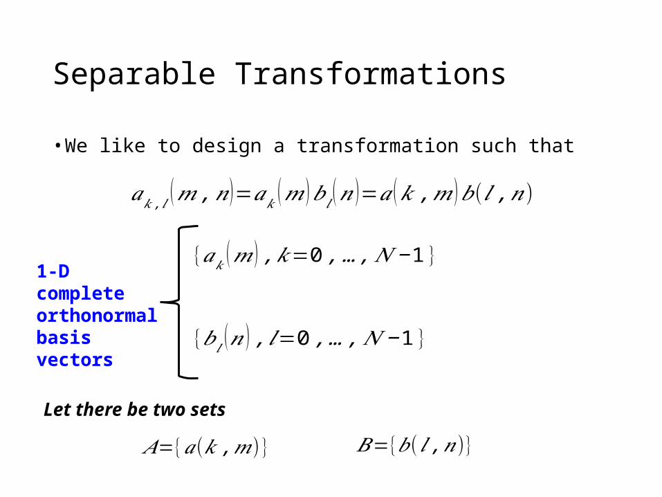
• We like to design a transformation such that
𝑎𝑘 ,𝑙 (𝑚 ,𝑛)=𝑎𝑘 (𝑚 )𝑏𝑙 (𝑛 )=𝑎 (𝑘 ,𝑚 )𝑏( 𝑙 ,𝑛)
{𝑎𝑘 (𝑚 ) ,𝑘=0 ,…,𝑁−1}
{𝑏𝑙 (𝑛) , 𝑙=0 ,…,𝑁−1 }
𝐴={𝑎(𝑘 ,𝑚)} 𝐵={𝑏 (𝑙 ,𝑛)}
Let there be two sets
1-D complete orthonormal basis vectors

Separable Transformations
𝐴 𝐴∗𝑇=𝐴∗𝑇 𝐴=𝐼
Assumption: the separable matrices be same, then
𝐵𝐵∗𝑇=𝐵∗𝑇 𝐵=𝐼
𝑣 (𝑘 , 𝑙 )=∑𝑚=0
𝑁−1
∑𝑛=0
𝑁− 1
𝑎 (𝑘 ,𝑚 )𝑢 (𝑚 ,𝑛)𝑎(𝑙 ,𝑛)
What would be v in matrix notation?
𝑽=𝑨𝑼 𝑨𝑻

Reverse transformations
1N
0k
1N
0l
** ron),(l,al)v(k,m)(k,an)u(m, *T* VAAU
For non-square matrices
V A UAM N
U A VAM*T
N*T
V AUA , V A[AU]T T T

=
[𝑎 (0 ,0 ) ⋯ 𝑎 (0 ,𝑚 ) ⋯ 𝑎 (0 ,𝑁−1 )
⋮ ⋯ ⋯ ⋯ ⋮𝑎 (𝑘 ,0 ) ⋯ 𝑎(𝑘 ,𝑚) ⋯ 𝑎(𝑘 ,𝑁−1)
⋮ … … … ⋮𝑎(𝑁−1,0) … 𝑎(𝑁−1 ,𝑚) … 𝑎(𝑁−1 ,𝑁−1)
]×[
𝑢 (0 ,0 ) ⋯ 𝑢 (0 ,𝑛) ⋯ 𝑢 (0 ,𝑁−1 )⋮ ⋯ ⋯ ⋯ ⋮
𝑢 (𝑚 ,0 ) ⋯ 𝑢(𝑚 ,𝑛) … 𝑢 (𝑚 ,𝑁−1)⋮ … … … ⋮
𝑢(𝑁−1,0) … 𝑢(𝑁−1 ,𝑙) … 𝑢(𝑁−1 ,𝑁−1)]×
[𝑎 (0 ,0 ) ⋯ 𝑎 (0 ,𝑛) ⋯ 𝑎 (0 ,𝑁−1 )
⋮ ⋯ ⋯ ⋯ ⋮𝑎 (𝑙 ,0 ) ⋯ 𝑎(𝑙 ,𝑛) ⋯ 𝑎(𝑙 ,𝑁−1)
⋮ … … … ⋮𝑎(𝑁−1,0) … 𝑎(𝑁−1 ,𝑛) … 𝑎(𝑁−1 ,𝑁−1)
]
Computational complexity
O(N3)

Example
𝐴=12 [√ 3 1−1 √3 ] 𝑈=[2 3
1 2]𝑉=𝐴𝑈 𝐴𝑇
𝑉=12 [√ 3 1−1 √3 ][2 3
1 2] 12 [√ 3 −11 √3 ]
𝑉=[2+√3 20 2−√ 3]

Inverse transforms
𝑉=[2+√3 20 2−√ 3] 𝐴∗𝑇=1
2 [√ 3 −11 √3 ]
𝑢 (1,0 )=∑𝑘=0
1
∑𝑙=0
1
𝑎∗ (𝑘 ,1 )𝑣 (𝑘 , 𝑙 )𝑎∗( 𝑙 ,0)
1N
0k
1N
0l
** ron),(l,al)v(k,m)(k,an)u(m, *T* VAAU
Kronecker Products
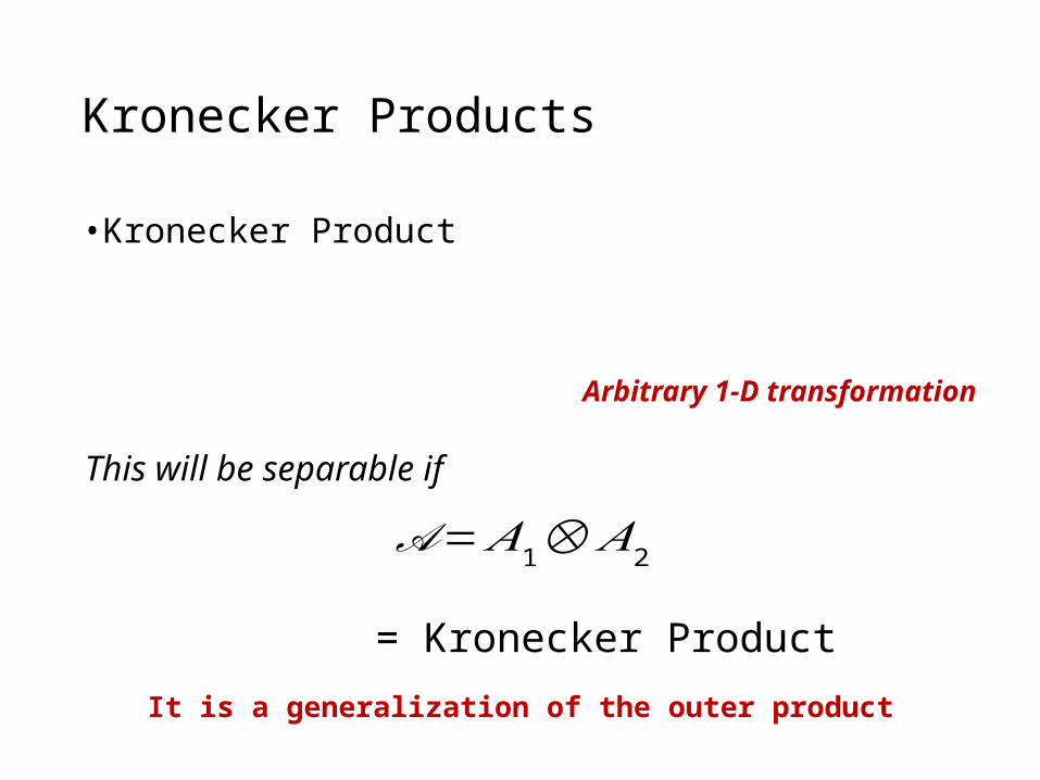
• Kronecker Product
Arbitrary 1-D transformation
This will be separable if𝒜=𝐴1⨂ 𝐴2
= Kronecker Product
It is a generalization of the outer product
Kronecker Products
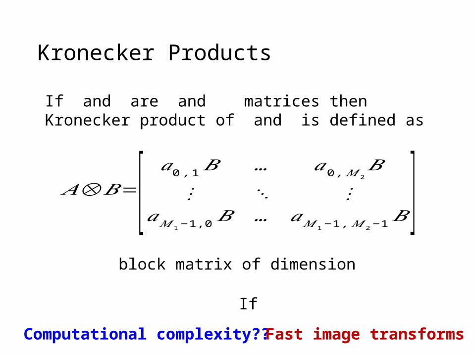
𝐴⨂𝐵=[ 𝑎0 , 1𝐵 … 𝑎0 ,𝑀2𝐵
⋮ ⋱ ⋮𝑎𝑀1−1,0
𝐵 … 𝑎𝑀 1−1 ,𝑀 2−1𝐵]
If and are and matrices then Kronecker product of and is defined as
block matrix of dimension
If
Computational complexity?? Fast image transforms
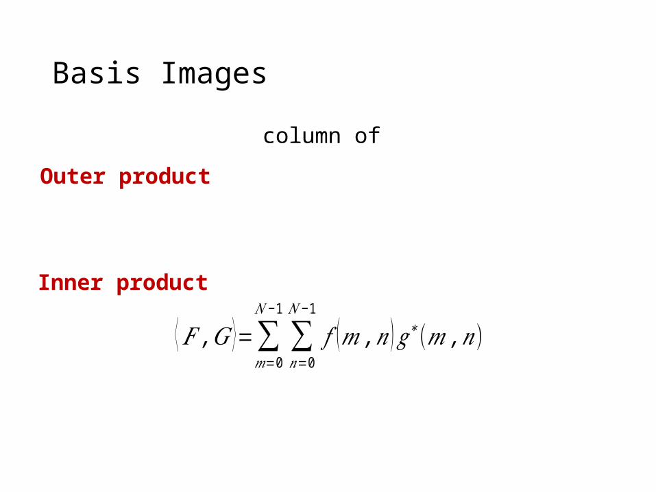
Basis Images
column of
Outer product
Inner product
⟨ 𝐹 ,𝐺 ⟩=∑𝑚=0
𝑁 −1
∑𝑛=0
𝑁−1
𝑓 (𝑚 ,𝑛 )𝑔∗(𝑚 ,𝑛)

Basis Images
Imagine originala
=
=
V(1,3)
+ + +
+ + + + + +
+ + + + … +
V(1,5) V(1,7) V(1,9)
V(1,13) V(1,15) V(2,1) V(2,9) V(3,1) V(3,5)
V(5,1) V(5,2) V(5,6) V(5,8) V(16,15)
Imagine aproximata
Keeping only 50% of coefficients
Thank youNext Lecture: Discrete Fourier Transform


