CSC 261/461 – Database SystemsLecture 17

Fall 2017

CSC261,Fall2017

Announcement

• Quiz 6 – Due: Tonight at 11:59 pm

• Project 1 Milepost 3 – Due: Nov 10

• Project 2 Part 2 (Optional)– Due: Nov 15

CSC261,Fall2017

The IO Model & External Sorting

CSC261,Fall2017

Today’s Lecture

1. Chapter16(DiskStorage,FileStructureandHashing)2. Chapter17(Indexing)

CSC261,Fall2017

Self-Study

• Buffering of Blocks– Pin Count and Dirty Bit– Buffer Replacement Strategies• Least recently used (LRU)• Clock Policy• First in First Out (FIFO)• MRU (Most recently used)

CSC261,Fall2017

RECORDS AND FILES

CSC261,Fall2017

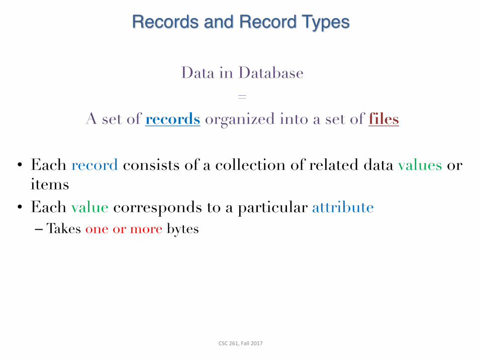
Records and Record Types

Data in Database =

A set of records organized into a set of files

• Each record consists of a collection of related data values or items

• Each value corresponds to a particular attribute– Takes one or more bytes

CSC261,Fall2017

Fixed Length Records vs Variable Length Records

• Fig 16.5 (from textbook)

CSC261,Fall2017

Record Blocking

• Block Size = 𝐵bytes• Fixed Record Size = 𝑅 bytes

• With 𝐵 > 𝑅:– Records per block = 𝑏𝑓𝑟 = ⌊+

,⌋

– Unused space per block = 𝐵– 𝑏𝑓𝑟 ∗ 𝑅 = B mod R

• Number of Blocks required = ⌈ 𝑅/𝑏𝑓𝑟 ⌉

• Two scenarios:– Spanned: records can span more than one block– Unspanned: records can’t span more than one block

CSC261,Fall2017

Unspanned vs Spanned

Unspanned

Spanned

CSC261,Fall2017

Heap Files vs Sorted Files

• Insertion • (Heap vs Sorted)• For Sorted files: Overflow

• Deletion – Deletion Marker

• Modifying– For Sorted files: May consist of Deletion and Insertion

• Searching– How many block access?– (by record number) What if the records are numbered and are of

fixed size?– Searching by range (Heap vs Sorted)

CSC261,Fall2017

Another variety

• Another type of files beyond: – Heap Files and Sorted Files

–Hash Files

CSC261,Fall2017

2. HASHING TECHNIQUES

CSC261,Fall2017

“IF YOU DON’T FIND IT IN THE INDEX, LOOK VERY CAREFULLY THROUGH THE ENTIRE CATALOG”

- Sears, Roebuck and Co., Consumers Guide, 1897

CSC261,Fall2017

HASING – GENERAL IDEAS

- Hashing first proposed by Arnold Dumey (1956)- Hash codes- Chaining- Open addressing

CSC261,Fall2017

Example

JavaHashCode

CSC261,Fall2017

Top level view

Arbitraryobjects(strings,doubles,ints)

n Objectsactuallyused

Hashcode

{0,1,…,m-1}int withwiderange

h(object)

Compressionfunction

m

Wewillalsocallthisthehashfunction

CSC261,Fall2017

Example (Once again!)

JavaHashCode

CSC261,Fall2017

True / False

• Unequal objects must have different hash codes

• Objects with the same hash code must be equal

• Both Wrong –We would like this but it’s impossible to achieve – Still possible for a particular set of values but impossible if input

values are unknown prior to applying the hashcode.

CSC261,Fall2017

Good Hash Function

• If key1 ≠ key2, then it’s extremely unlikely that h(key1) = h(key2)– Collision problem!

• Pigeonhole principle– K+1 pigeons, K holes à at least one hole with ≥ 2 pigeons

CSC261,Fall2017

Division method

• How does this function perform for different m?h(s) = s mod m

CSC261,Fall2017

COLLISION RESOLUTION

Separate chaining

Open addressing

CSC261,Fall2017

Separate Chaining

Turing

Cantor

Knuth

Karp

Dijkstra

Index Pointer

0

1

2

3

4

Turing Knuth Dijkstra

Karp Cantor

CSC261,Fall2017

Open Addressing

• Store all entries in the hash table itself, no pointer to the “outside”– If a particular index i is full, try the next index (i+C) where C is a

constant.

• Advantage– Less space waste– Perhaps good cache usage

• Disadvantage–More complex collision resolution– Slower operations

CSC261,Fall2017

Open Addressing

Turing

Cantor

Knuth

Karp

Dijkstra

Index Pointer

0

1

2

3

4

5

6

7

Turing

Knuth

DijkstraKarp

Cantor

h(“Knuth”,0)h(“Knuth”,1)

h(“Karp”,0) h(“Karp”,1)

h(“Dijkstra”,0)

h(“Dijkstra”,1)

h(“Dijkstra”,2)

C=2

CSC261,Fall2017

External Hashing

• Hashing for disk files

• Target address space is made of buckets

• Hashing function maps a key into relative bucket number

• Convert the bucket number into corresponding disk block address

CSC261,Fall2017

Bucket Number to Disk Block address

CSC261,Fall2017

Bucket Number to Disk Block address

CSC261,Fall2017

REVIEW

CSC261,Fall2017

What Did We Learn

• Disk Storage – Hardware Description of Disk Devices • Sections to study: 16.2.1 and 16.2.2

• Buffering of Blocks • Buffer Management• Buffer Replacement Strategies• Sections to study: 16.3

• Placing File Records on Disk• Records and Record Types• Fixed-Length, Variable-Length, Spanned, Unspanned• Sections to study: 16.4.1 to 16.4.4

CSC261,Fall2017

What did we learn

• Operations on Files• Insert, Modify, and Delete• And others. • Sections to study: 16.5

• Heap Files vs Sorted Files• Sections to study: 16.6 and 16.7

• Hash Files• Internal Hashing and External Hashing• Sections to study: 16.8.1 and 16.8.2

CSC261,Fall2017

INDEXING

CSC261,Fall2017

Types of Indexing

• Primary Indexes

• Clustering Indexes

• Secondary Indexes

• Multilevel Indexes– Dynamic Multilevel Indexes

• Hash Indexes

CSC261,Fall2017

What you will learn about in this section

1. Indexes:Motivation

2. Indexes:Basics

CSC261,Fall2017

Index Motivation

• Suppose we want to search for people of a specific age

• First idea: Sort the records by age… we know how to do this fast!

• How many IO operations to search over N sorted records?– Simple scan: O(N)– Binary search: O(𝐥𝐨𝐠𝟐 𝑵)

Person(name, age)

Couldwegetevencheapersearch?E.g.gofrom𝐥𝐨𝐠𝟐 𝑵à 𝐥𝐨𝐠𝟐𝟎𝟎 𝑵?

CSC261,Fall2017

Index Motivation

• What about if we want to insert a new person, but keep the list sorted?

• We would have to potentially shift N records, requiring up to ~ 2*N/P IO operations (where P = # of records per page)!– We could leave some “slack” in the pages…

4,5 6,71,3 3,4 5,61,2

2

7,

Couldwegetfasterinsertions?

CSC261,Fall2017

Index Motivation

• What about if we want to be able to search quickly along multiple attributes (e.g. not just age)?–We could keep multiple copies of the records, each sorted

by one attribute set… this would take a lot of space

Canwegetfastsearchovermultipleattribute(sets)withouttakingtoomuchspace?

We’llcreateseparatedatastructurescalledindexes toaddressallthesepoints

CSC261,Fall2017

Further Motivation for Indexes: NoSQL!

• NoSQL engines are (basically) just indexes!

– A lot more is left to the user in NoSQL… one of the primary remaining functions of the DBMS is still to provide index over the data records, for the reasons we just saw!

– Sometimes use B+ Trees, sometimes hash indexes

IndexesarecriticalacrossallDBMStypes

CSC261,Fall2017

Indexes: High-level

• An index on a file speeds up selections on the search key fields for the index.– Search key properties

• Any subset of fields• is not the same as key of a relation

• Example: Onwhichattributeswouldyoubuild

indexes?Product(name, maker, price)

CSC261,Fall2017

More precisely

• An index is a data structure mapping search keys to sets of rows in a database table

– Provides efficient lookup & retrieval by search key value-usually much faster than searching through all the rows of the database table

• An index can store:– Full rows it points to (primary index) or – Pointers to those rows (secondary index)

CSC261,Fall2017

Operations on an Index

• Search: Quickly find all records which meet some conditionon the search key attributes–More sophisticated variants as well. Why?

Indexingisonethemostimportantfeaturesprovidedbyadatabaseforperformance

CSC261,Fall2017

Conceptual Example

Whatifwewanttoreturnallbookspublishedafter1867?Theabovetablemightbeveryexpensivetosearchoverrow-by-row…

SELECT *FROM Russian_NovelsWHERE Published > 1867

BID Title Author Published Full_text

001 WarandPeace Tolstoy 1869 …

002 CrimeandPunishment

Dostoyevsky 1866 …

003 AnnaKarenina Tolstoy 1877 …

Russian_Novels

CSC261,Fall2017

Conceptual Example

BID Title Author Published Full_text

001 WarandPeace Tolstoy 1869 …

002 CrimeandPunishment

Dostoyevsky 1866 …

003 AnnaKarenina Tolstoy 1877 …

Published BID

1866 002

1869 001

1877 003

Maintainanindexforthis,andsearchoverthat!

Russian_NovelsBy_Yr_Index

Whymightjustkeepingthetablesortedbyyearnotbegoodenough?

CSC261,Fall2017

Conceptual Example

BID Title Author Published Full_text

001 WarandPeace Tolstoy 1869 …

002 CrimeandPunishment

Dostoyevsky 1866 …

003 AnnaKarenina Tolstoy 1877 …

Published BID

1866 002

1869 001

1877 003

Indexesshownhereastables,butinrealitywewillusemoreefficientdatastructures…

Russian_NovelsBy_Yr_Index

Author Title BID

Dostoyevsky Crime andPunishment

002

Tolstoy AnnaKarenina 003

Tolstoy War andPeace 001

By_Author_Title_Index Canhavemultipleindexestosupportmultiplesearchkeys

CSC261,Fall2017

Covering Indexes

Published BID

1866 002

1869 001

1877 003

By_Yr_Index

Wesaythatanindexiscovering foraspecificquery iftheindexcontainsalltheneededattributes-meaningthequerycanbeansweredusingtheindexalone!

The“needed”attributesaretheunionofthoseintheSELECTandWHEREclauses…

SELECT Published, BIDFROM Russian_NovelsWHERE Published > 1867

Example:

CSC261,Fall2017

TYPES OF INDEXES

CSC261,Fall2017

Types of Indexing

• Primary Indexes

• Clustering Indexes

• Secondary Indexes

• Multilevel Indexes– Dynamic Multilevel Indexes

• Hash Indexes

CSC261,Fall2017

Primary Indexes: Index for Sorted (Ordered) Files

CSC261,Fall2017

Clustering Indexes (Index for Sorted (on non-key) Files)

CSC261,Fall2017

Secondary Indexes (on a key field)

• Secondary means of accessing a data file

• File records could be ordered, unordered, or hashed

CSC261,Fall2017

Secondary Indexes (on a non-key field)Extra level of indirection

• Provides logical ordering– Though records are not

physically ordered

CSC261,Fall2017

High-level Categories of Index Types

• Multilevel Indexes– Very good for range queries, sorted data– Some old databases only implemented B-Trees– We will mostly look at a variant called B+ Trees

• Hash Tables – Very good for searching

Realdifferencebetweenstructures:costsofopsdetermineswhichindexyoupickandwhy

CSC261,Fall2017

MULTILEVEL INDEXES

CSC261,Fall2017

What you will learn about in this section

1. ISAM

2. B+Tree

CSC261,Fall2017

1. ISAM

CSC261,Fall2017

ISAM

• Indexed Sequential Access Method

– For an index with𝑏9blocks• Earlier: log=b?block

access• Now: log@Ab? block

access• (𝑓𝑜 = 𝑓𝑎𝑛𝑜𝑢𝑡)

CSC261,Fall2017

1. B+ TREES

CSC261,Fall2017

What you will learn about in this section

1. B+Trees:Basics

2. B+Trees:Design&Cost

3. ClusteredIndexes

CSC261,Fall2017

B+ Trees

• Search trees – B does not mean binary!

• Idea in B Trees:–make 1 node = 1 physical page– Balanced, height adjusted tree (not the B either)

• Idea in B+ Trees:–Make leaves into a linked list (for range queries)

CSC261,Fall2017

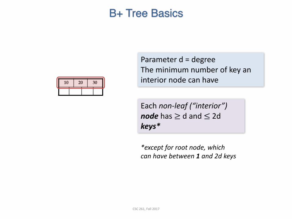
B+ Tree Basics

10 20 30

Eachnon-leaf(“interior”)node has≥ dand≤2dkeys*

*exceptforrootnode,whichcanhavebetween1and2dkeys

Parameterd=degreeTheminimumnumberofkeyaninteriornodecanhave

CSC261,Fall2017

B+ Tree Basics

10 20 30

k<10

10≤ 𝑘<20

20≤ 𝑘<3030≤ 𝑘

Thenkeysinanodedefinen+1ranges

CSC261,Fall2017

B+ Tree Basics

10 20 30

Non-leaforinternalnode

22 25 28

Foreachrange,inanon-leafnode,thereisapointer toanothernodewithkeysinthatrange

CSC261,Fall2017

B+ Tree Basics

10 20 30

Leafnodesalsohavebetweendand2dkeys,andaredifferentinthat:

22 25 28 29

Leaf nodes

32 34 37 38

Non-leaforinternalnode

12 17

CSC261,Fall2017

B+ Tree Basics

10 20 30

22 25 28 29

Leaf nodes

32 34 37 38

Non-leaforinternalnode

12 17

Leafnodesalsohavebetweendand2dkeys,andaredifferentinthat:

Theirkeyslotscontainpointerstodatarecords

21 22 27 28 30 33 35 3715

11

CSC261,Fall2017

B+ Tree Basics

10 20 30

22 25 28 29

Leaf nodes

32 34 37 38

Non-leaforinternalnode

12 17

21 22 27 28 30 33 35 3715

11

Leafnodesalsohavebetweendand2dkeys,andaredifferentinthat:

Theirkeyslotscontainpointerstodatarecords

Theycontainapointertothenextleafnodeaswell,forfastersequentialtraversal

CSC261,Fall2017

B+ Tree Basics

10 20 30

22 25 28 29

Leaf nodes

32 34 37 38

Non-leaforinternalnode

12 17

Notethatthepointersattheleaflevelwillbetotheactualdatarecords(rows).

Wemighttruncatetheseforsimplerdisplay(asbefore)…

Name:JohnAge:21

Name:JakeAge:15

Name:BobAge:27

Name:SallyAge:28

Name:SueAge:33

Name:JessAge:35

Name:AlfAge:37Name:Joe

Age:11

Name:BessAge:22

Name:SalAge:30

CSC261,Fall2017

Some finer points of B+ Trees

CSC261,Fall2017

Searching a B+ Tree

• For exact key values:–Start at the root–Proceed down, to the leaf

• For range queries:–As above–Then sequential traversal

SELECT nameFROM peopleWHERE age = 25

SELECT nameFROM peopleWHERE 20 <= ageAND age <= 30

CSC261,Fall2017

B+ Tree Exact Search Animation

80

20 60 100 120 140

10 15 18 20 30 40 50 60 65 80 85 90

10 12 15 20 28 30 40 60 63 80 84 89

K=30?

30<80

30in[20,60)

Tothedata!

Notallnodespictured

30in[30,40)

CSC261,Fall2017

B+ Tree Range Search Animation

80

20 60 100 120 140

10 15 18 20 30 40 50 60 65 80 85 90

10 12 15 20 28 30 40 59 63 80 84 89

Kin[30,85]?

30<80

30in[20,60)

Tothedata!

Notallnodespictured

30in[30,40)

CSC261,Fall2017

B+ Tree Design

• How large is d?

• Example:– Key size = 4 bytes– Pointer size = 8 bytes– Block size = 4096 bytes

• We want each node to fit on a single block/page– 2d x 4 + (2d+1) x 8 <= 4096 à d <= 170

CSC261,Fall2017

B+ Tree: High Fanout = Smaller & Lower IO

• As compared to e.g. binary search trees, B+ Trees have high fanout(between d+1 and 2d+1)

• This means that the depth of the tree is small à getting to any element requires very few IO operations!– Also can often store most or all of the

B+ Tree in main memory!

Thefanout isdefinedasthenumberofpointerstochildnodescomingoutofanode

Notethatfanout isdynamic-we’lloftenassumeit’sconstantjusttocomeupwithapproximateeqns!

CSC261,Fall2017

Simple Cost Model for Search• Let:

– f = fanout, which is in [d+1, 2d+1] (we’ll assume it’s constant for our cost model…)– N = the total number of pages we need to index– F = fill-factor (usually ~= 2/3)

• Our B+ Tree needs to have room to index N / F pages!– We have the fill factor in order to leave some open slots for faster insertions

• What height (h) does our B+ Tree need to be?– h=1 à Just the root node- room to index f pages– h=2 à f leaf nodes- room to index f2 pages– h=3 à f2 leaf nodes- room to index f3 pages– …– h à fh-1 leaf nodes- room to index fh pages!

àWeneedaB+Treeofheighth= logK

LM

CSC261,Fall2017

Fast Insertions & Self-Balancing

– Same cost as exact search– Self-balancing: B+ Tree remains balanced (with respect to

height) even after insert

B+Treesalso(relatively)fastforsingleinsertions!However,canbecomebottleneckifmanyinsertions(iffill-

factorslackisusedup…)CSC261,Fall2017

Insertion

• Perform a search to determine what bucket the new record should go into.

• If the bucket is not full (at most (b-1) entries after the insertion), add the record.

• Otherwise, split the bucket.– Allocate new leaf and move half the bucket's elements to the new bucket.– Insert the new leaf's smallest key and address into the parent.– If the parent is full, split it too.

• Add the middle key to the parent node.– Repeat until a parent is found that need not split.

• If the root splits, create a new root which has one key and two pointers. (That is, the value that gets pushed to the new root gets removed from the original node)

• Note: B-trees grow at the root and not at the leave

CSC261,Fall2017

Insertion (Insert 85)

CSC261,Fall2017

b=f=branchingfactor/fan-out=3

20 40 80 90

40 80

Insertion (Insert 85)

CSC261,Fall2017

b=f=branchingfactor/fan-out=3

20 40 80 90

40 80

85

Thisiswhatwewouldlike.Butthemaximumnumberofkeysinanynodeis(3-1)=2So,split.

Insertion (Insert 85)

CSC261,Fall2017

b=f=branchingfactor/fan-out=3

20 40 80

40 80

85

Allocatenewleafandmovehalfthebucket'selementstothenewbucket.

90

Insertion (Insert 85)

CSC261,Fall2017

b=f=branchingfactor/fan-out=3

20 40 80

40 80

85

Insertthenewleaf'ssmallestkeyandaddressintotheparent.

90

85

Insertion (Insert 85)

CSC261,Fall2017

b=f=branchingfactor/fan-out=3

20 40 80

40 80

85

Thisisnotallowed,astheparentisfull.Needtosplit

90

85

Insertion (Insert 85)

CSC261,Fall2017

b=f=branchingfactor/fan-out=3

20 40 80

40

80

85

Iftheparentisfull,splitittoo.

Addthemiddlekeytotheparentnode.

Repeatuntilaparentisfoundthatneedsnospliting

90

85

Insertion (Insert 85)

CSC261,Fall2017

b=f=branchingfactor/fan-out=3

20 40 80

40

80

85

Iftherootsplits,createanewrootwhichhasonekeyandtwopointers.

(Thatis,thevaluethatgetspushedtothenewrootgetsremovedfromtheoriginalnode)

90

85

Deletion

• Start at root, find leaf L where entry belongs.• Remove the entry.– If L is at least half-full, done!– If L has fewer entries than it should,

• If sibling (adjacent node with same parent as L) is more than half-full, re-distribute, borrowing an entry from it.

• Otherwise, sibling is exactly half-full, so we can merge L and sibling.• If merge occurred, must delete entry (pointing to L or sibling)

from parent of L.• Merge could propagate to root, decreasing height.

• https://www.cs.usfca.edu/~galles/visualization/BPlusTree.html

• The degree in this visualization is actually fan-out f or branching factor b.

CSC261,Fall2017

• Find 86

CSC261,Fall2017

• Delete it

CSC261,Fall2017

• Stealing from right sibling (redistribute).• Modify the parent node

CSC261,Fall2017

• Finally,

CSC261,Fall2017

Acknowledgement

• Some of the slides in this presentation are taken from the slides provided by the authors.

• Many of these slides are taken from cs145 course offered byStanford University.

CSC261,Fall2017