69
CSC373 Week 7: Linear Programming 373F21 - Nisarg Shah 1 Illustration Courtesy: Kevin Wayne & Denis Pankratov

CSC373
Week 7: Linear Programming
373F21 - Nisarg Shah 1
Illustration Courtesy: Kevin Wayne & Denis Pankratov

Recap
373F21 - Nisarg Shah 2
• Network flow
➢ Ford-Fulkerson algorithm
o Ways to make the running time polynomial
➢ Correctness using max-flow, min-cut
➢ Applications:
o Edge-disjoint paths
o Multiple sources/sinks
o Circulation
o Circulation with lower bounds
o Survey design
o Image segmentation
o Profit maximization
Brewery Example
373F21 - Nisarg Shah 3
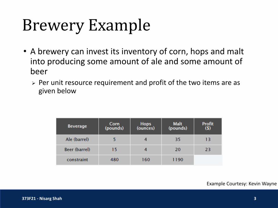
• A brewery can invest its inventory of corn, hops and malt into producing some amount of ale and some amount of beer➢ Per unit resource requirement and profit of the two items are as
given below
Example Courtesy: Kevin Wayne

Brewery Example
373F21 - Nisarg Shah 4
• Suppose it produces 𝐴units of ale and 𝐵 units of beer
• Then we want to solve this program:
Linear Function
373F21 - Nisarg Shah 5
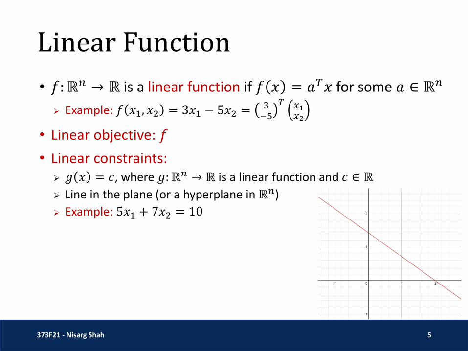
• 𝑓:ℝ𝑛 → ℝ is a linear function if 𝑓 𝑥 = 𝑎𝑇𝑥 for some 𝑎 ∈ ℝ𝑛
➢ Example: 𝑓 𝑥1, 𝑥2 = 3𝑥1 − 5𝑥2 =3−5
𝑇 𝑥1𝑥2
• Linear objective: 𝑓
• Linear constraints:➢ 𝑔 𝑥 = 𝑐, where 𝑔:ℝ𝑛 → ℝ is a linear function and 𝑐 ∈ ℝ
➢ Line in the plane (or a hyperplane in ℝ𝑛)
➢ Example: 5𝑥1 + 7𝑥2 = 10
Linear Function
373F21 - Nisarg Shah 6
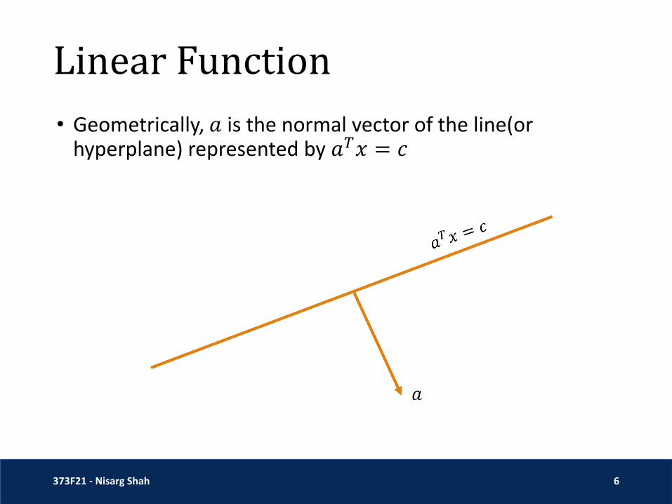
• Geometrically, 𝑎 is the normal vector of the line(or hyperplane) represented by 𝑎𝑇𝑥 = 𝑐

Linear Inequality
373F21 - Nisarg Shah 7
• 𝑎𝑇𝑥 ≤ 𝑐 represents a “half-space”

Linear Programming
373F21 - Nisarg Shah 8
• Maximize/minimize a linear function subject to linear equality/inequality constraints

Geometrically…
373F21 - Nisarg Shah 9

Back to Brewery Example
373F21 - Nisarg Shah 10

Back to Brewery Example
373F21 - Nisarg Shah 11

• Claim: Regardless of the objective function, there must be a vertex that is an optimal solution
Optimal Solution At A Vertex
373F21 - Nisarg Shah 12
Convexity
373F21 - Nisarg Shah 13
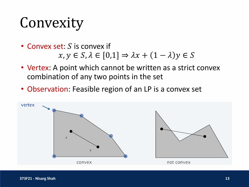
• Convex set: 𝑆 is convex if 𝑥, 𝑦 ∈ 𝑆, 𝜆 ∈ [0,1] ⇒ 𝜆𝑥 + 1 − 𝜆 𝑦 ∈ 𝑆
• Vertex: A point which cannot be written as a strict convex combination of any two points in the set
• Observation: Feasible region of an LP is a convex set
Optimal Solution At A Vertex
373F21 - Nisarg Shah 14
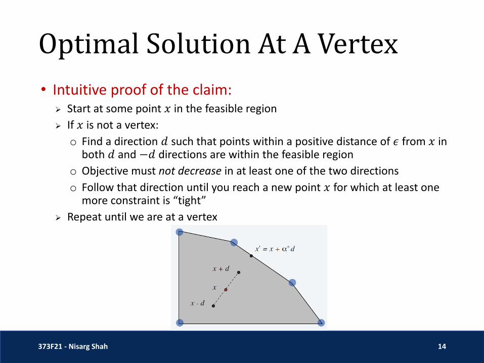
• Intuitive proof of the claim:➢ Start at some point 𝑥 in the feasible region
➢ If 𝑥 is not a vertex:
o Find a direction 𝑑 such that points within a positive distance of 𝜖 from 𝑥 in both 𝑑 and −𝑑 directions are within the feasible region
o Objective must not decrease in at least one of the two directions
o Follow that direction until you reach a new point 𝑥 for which at least one more constraint is “tight”
➢ Repeat until we are at a vertex
LP, Standard Formulation
373F21 - Nisarg Shah 15
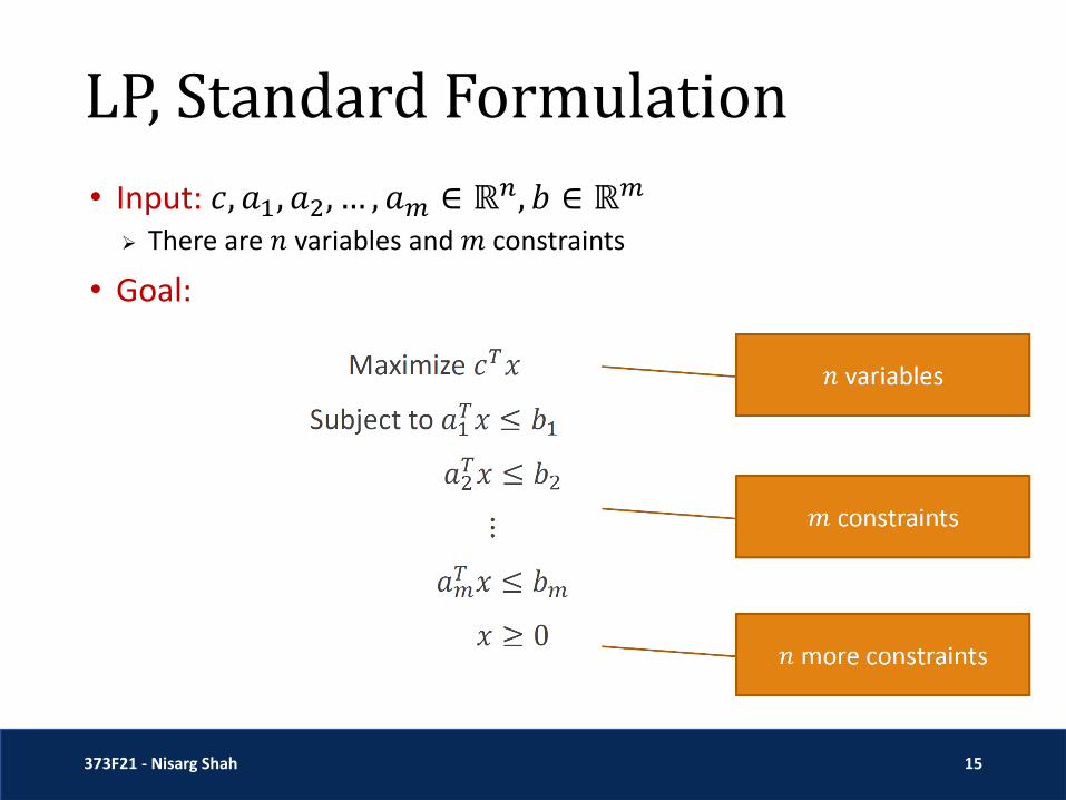
• Input: 𝑐, 𝑎1, 𝑎2, … , 𝑎𝑚 ∈ ℝ𝑛, 𝑏 ∈ ℝ𝑚
➢ There are 𝑛 variables and 𝑚 constraints
• Goal:

LP, Standard Matrix Form
373F21 - Nisarg Shah 16
• Input: 𝑐, 𝑎1, 𝑎2, … , 𝑎𝑚 ∈ ℝ𝑛, 𝑏 ∈ ℝ𝑚
➢ There are 𝑛 variables and 𝑚 constraints
• Goal:
Convert to Standard Form
373F21 - Nisarg Shah 17
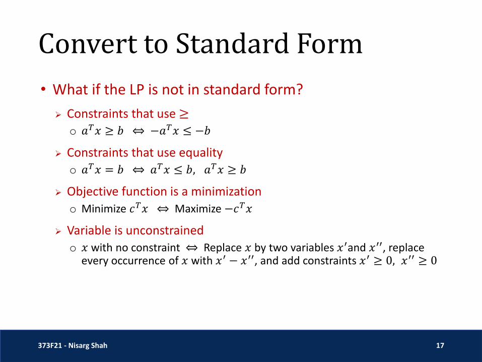
• What if the LP is not in standard form?
➢ Constraints that use ≥o 𝑎𝑇𝑥 ≥ 𝑏 ⇔ −𝑎𝑇𝑥 ≤ −𝑏
➢ Constraints that use equality
o 𝑎𝑇𝑥 = 𝑏 ⇔ 𝑎𝑇𝑥 ≤ 𝑏, 𝑎𝑇𝑥 ≥ 𝑏
➢ Objective function is a minimization
o Minimize 𝑐𝑇𝑥 ⇔ Maximize −𝑐𝑇𝑥
➢ Variable is unconstrained
o 𝑥 with no constraint ⇔ Replace 𝑥 by two variables 𝑥′and 𝑥′′, replace every occurrence of 𝑥 with 𝑥′ − 𝑥′′, and add constraints 𝑥′ ≥ 0, 𝑥′′ ≥ 0
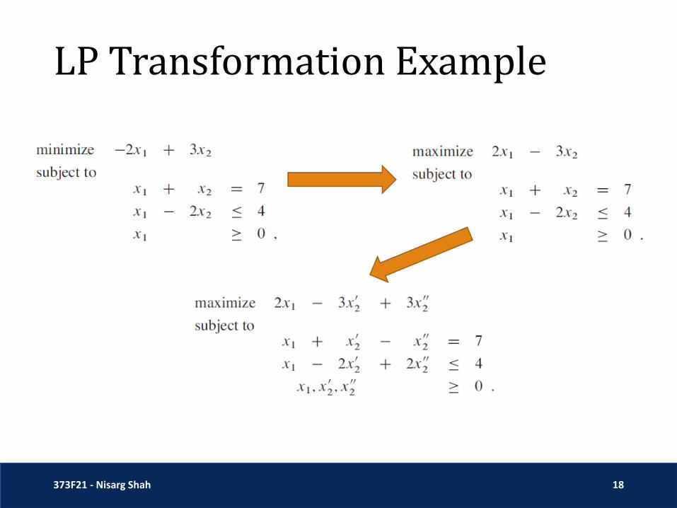
LP Transformation Example
373F21 - Nisarg Shah 18
Optimal Solution
373F21 - Nisarg Shah 19
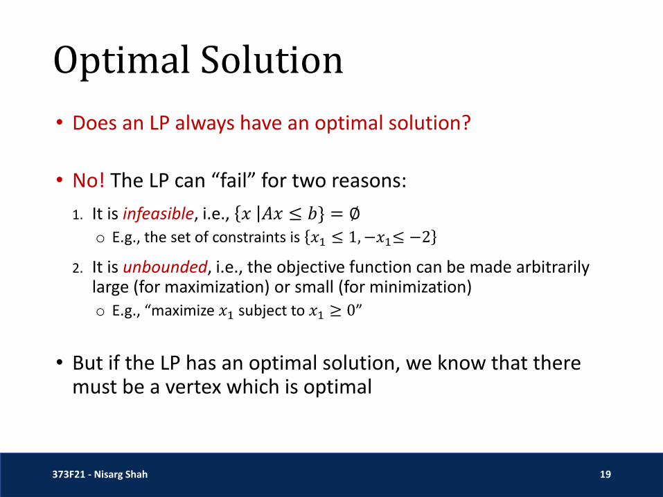
• Does an LP always have an optimal solution?
• No! The LP can “fail” for two reasons:
1. It is infeasible, i.e., 𝑥 𝐴𝑥 ≤ 𝑏} = ∅o E.g., the set of constraints is 𝑥1 ≤ 1,−𝑥1≤ −2
2. It is unbounded, i.e., the objective function can be made arbitrarily large (for maximization) or small (for minimization)o E.g., “maximize 𝑥1 subject to 𝑥1 ≥ 0”
• But if the LP has an optimal solution, we know that there must be a vertex which is optimal

Simplex Algorithm
373F21 - Nisarg Shah 20
• Simple algorithm, easy to specify geometrically
• Worst-case running time is exponential
• Excellent performance in practice

Simplex: Geometric View
373F21 - Nisarg Shah 21
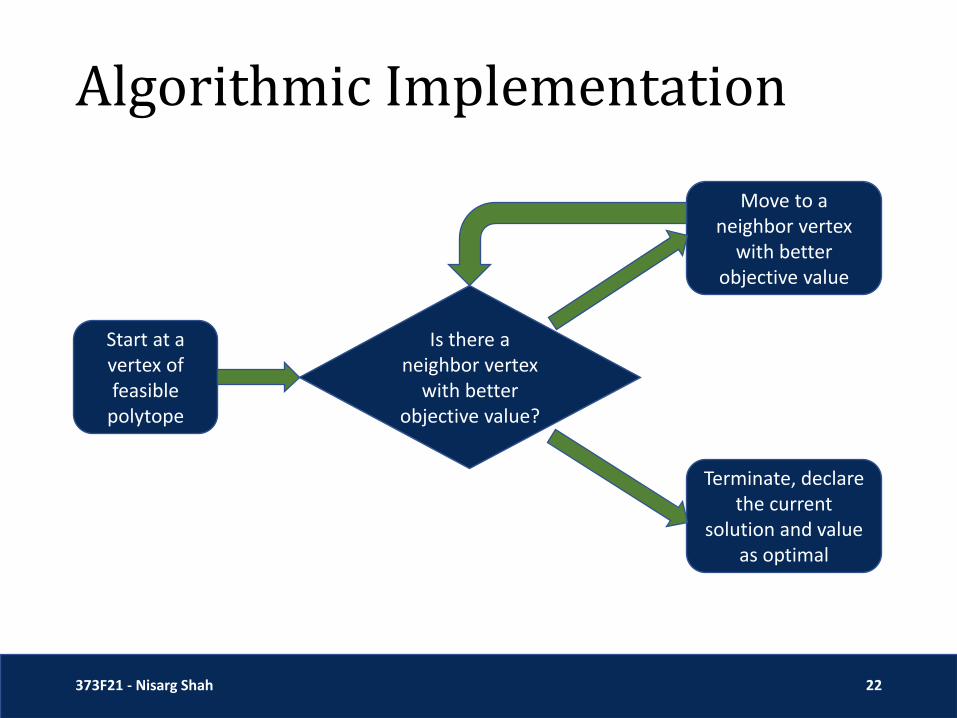
Algorithmic Implementation
373F21 - Nisarg Shah 22
Start at a vertex of feasible
polytope
Move to a neighbor vertex
with better objective value
Terminate, declare the current
solution and value as optimal
Is there a neighbor vertex
with better objective value?
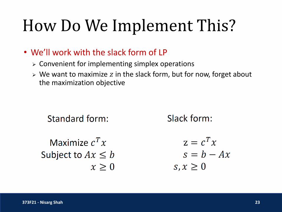
How Do We Implement This?
373F21 - Nisarg Shah 23
• We’ll work with the slack form of LP➢ Convenient for implementing simplex operations
➢ We want to maximize 𝑧 in the slack form, but for now, forget about the maximization objective

Slack Form
373F21 - Nisarg Shah 24
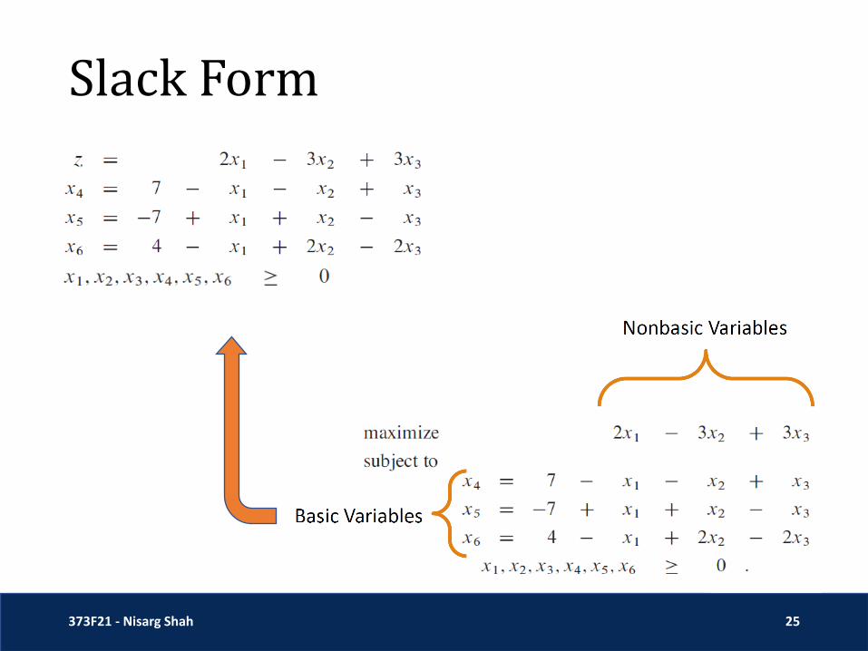
Slack Form
373F21 - Nisarg Shah 25

Simplex: Step 1
373F21 - Nisarg Shah 26
• Start at a feasible vertex➢ How do we find a feasible vertex?
➢ For now, assume 𝑏 ≥ 0 (that is, each 𝑏𝑖 ≥ 0)o In this case, 𝑥 = 0 is a feasible vertex.
o In the slack form, this means setting the nonbasic variables to 0
➢ We’ll later see what to do in the general case
Simple: Step 2
373F21 - Nisarg Shah 27
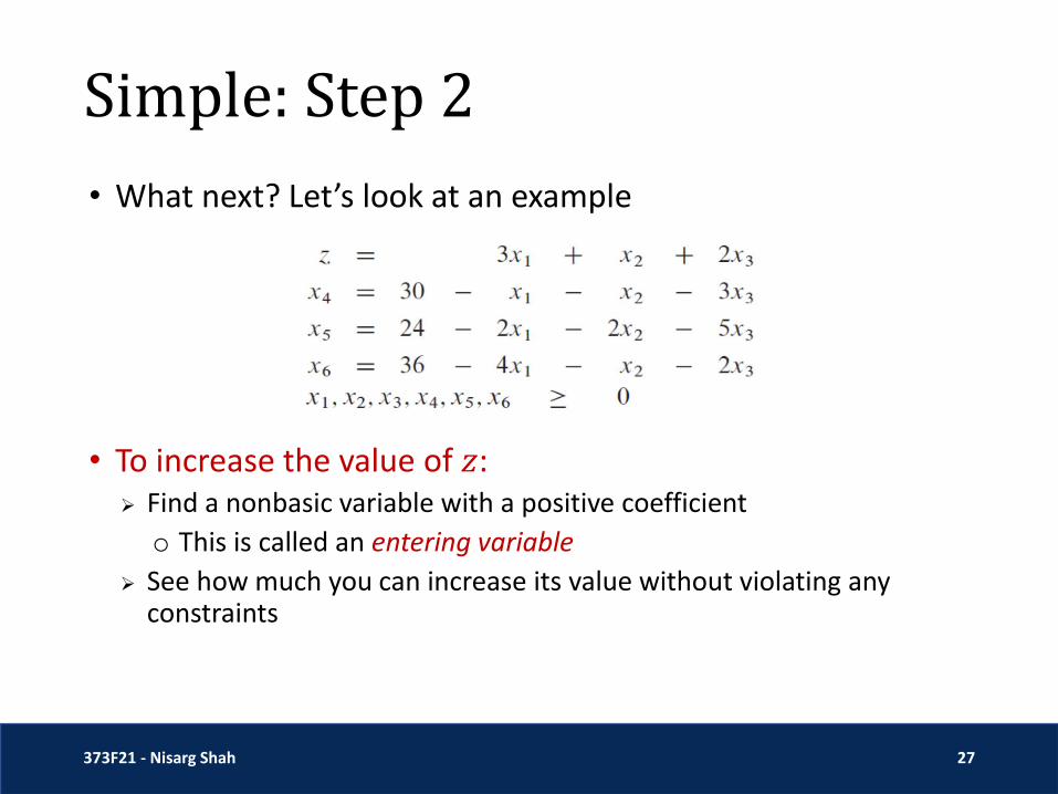
• What next? Let’s look at an example
• To increase the value of 𝑧:➢ Find a nonbasic variable with a positive coefficient
o This is called an entering variable
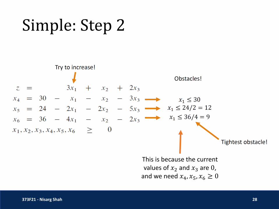
➢ See how much you can increase its value without violating any constraints
Simple: Step 2
373F21 - Nisarg Shah 28
This is because the current values of 𝑥2 and 𝑥3 are 0,
and we need 𝑥4, 𝑥5, 𝑥6 ≥ 0

Simple: Step 2
373F21 - Nisarg Shah 29
Tightest obstacle
➢ Solve the tightest obstacle for the nonbasic variable
𝑥1 = 9 −𝑥24−𝑥32−𝑥64
o Substitute the entering variable (called pivot) in other equations
o Now 𝑥1 becomes basic and 𝑥6 becomes non-basic
o 𝑥6 is called the leaving variable

Simplex: Step 2
373F21 - Nisarg Shah 30
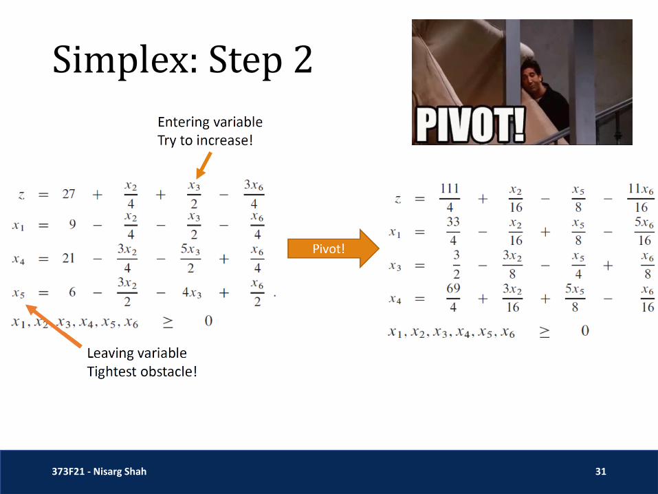
• After one iteration of this step:➢ The basic feasible solution (i.e., substituting 0 for all nonbasic
variables) improves from 𝑧 = 0 to 𝑧 = 27
• Repeat!
Simplex: Step 2
373F21 - Nisarg Shah 31

Simplex: Step 2
373F21 - Nisarg Shah 32

Simplex: Step 2
373F21 - Nisarg Shah 33
• There is no entering variable (nonbasic variable with positive coefficient) • What now? Nothing! We are done. • Take the basic feasible solution (𝑥3 = 𝑥5 = 𝑥6 = 0).• Gives the optimal value 𝑧 = 28• In the optimal solution, 𝑥1 = 8, 𝑥2 = 4, 𝑥3 = 0

Simplex Overview
373F21 - Nisarg Shah 34
Start at a vertex of feasible
polytope
Move to a neighbor vertex
with better objective value
Terminate, declare the current
solution and value as optimal
Is there a neighbor vertex
with better objective value?
Simplex Overview
373F21 - Nisarg Shah 35
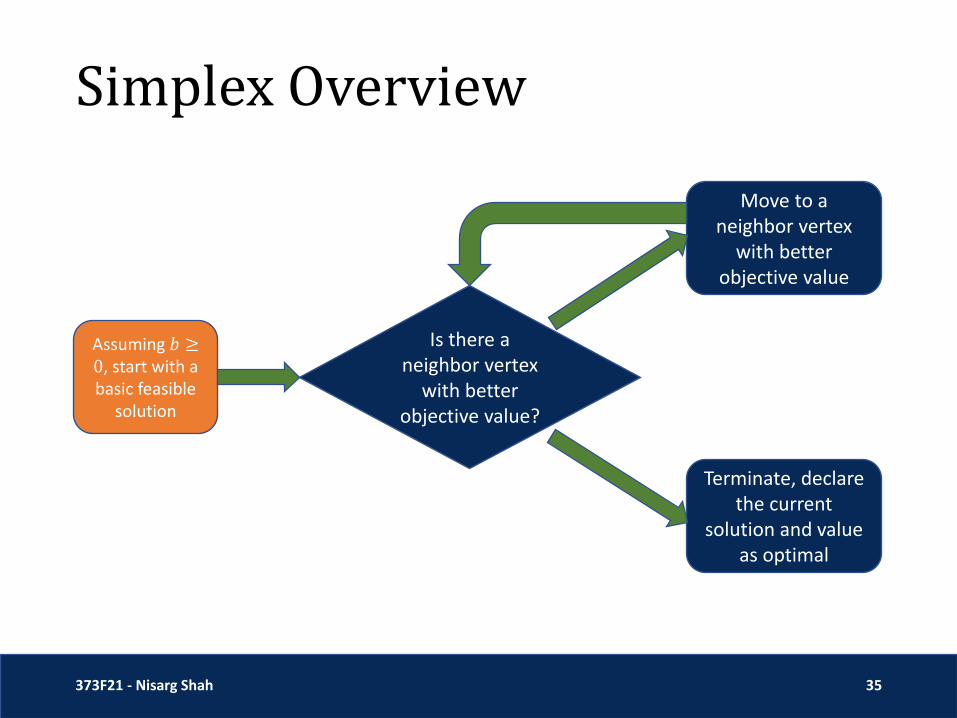
Assuming 𝑏 ≥0, start with a basic feasible
solution
Move to a neighbor vertex
with better objective value
Terminate, declare the current
solution and value as optimal
Is there a neighbor vertex
with better objective value?

Simplex Overview
373F21 - Nisarg Shah 36
Assuming 𝑏 ≥0, start with a basic feasible
solution
Move to a neighbor vertex
with better objective value
Terminate, declare the current
solution and value as optimal
Is there an entering variable
with positive coefficient?

Simplex Overview
373F21 - Nisarg Shah 37
Assuming 𝑏 ≥0, start with a basic feasible
solution
Pivot on a leaving variable
Terminate, declare the current
solution and value as optimal
Is there an entering variable
with positive coefficient?
Simplex Overview
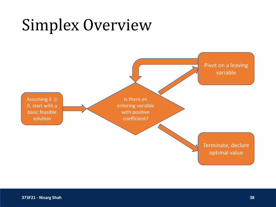
373F21 - Nisarg Shah 38
Assuming 𝑏 ≥0, start with a basic feasible
solution
Pivot on a leaving variable
Terminate, declare optimal value
Is there an entering variable
with positive coefficient?
Some Outstanding Issues
373F21 - Nisarg Shah 39
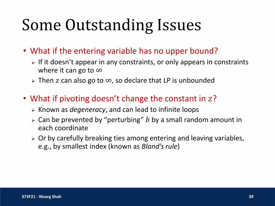
• What if the entering variable has no upper bound?➢ If it doesn’t appear in any constraints, or only appears in constraints
where it can go to ∞
➢ Then 𝑧 can also go to ∞, so declare that LP is unbounded
• What if pivoting doesn’t change the constant in 𝑧?➢ Known as degeneracy, and can lead to infinite loops
➢ Can be prevented by “perturbing” 𝑏 by a small random amount in each coordinate
➢ Or by carefully breaking ties among entering and leaving variables, e.g., by smallest index (known as Bland’s rule)

Some Outstanding Issues
373F21 - Nisarg Shah 40
• We assumed 𝑏 ≥ 0, and then started with the vertex 𝑥 = 0
• What if this assumption does not hold?
𝐿𝑃1
Max 𝑐𝑇𝑥
s.t. 𝑎1𝑇𝑥 ≤ 𝑏1
𝑎2𝑇𝑥 ≤ 𝑏2
⋮
𝑎𝑚𝑇 𝑥 ≤ 𝑏𝑚
𝑥 ≥ 0
𝐿𝑃2
Max 𝑐𝑇𝑥
s.t. 𝑎1𝑇𝑥 + 𝑠1 = 𝑏1
𝑎2𝑇𝑥 + 𝑠2 = 𝑏2
⋮
𝑎𝑚𝑇 𝑥 + 𝑠𝑚 = 𝑏𝑚
𝑥, 𝑠 ≥ 0
𝐿𝑃3
Max 𝑐𝑇𝑥
s.t. 𝑎1𝑇𝑥 + 𝑠1 = 𝑏1
−𝑎2𝑇𝑥 − 𝑠2 = −𝑏2
⋮
−𝑎𝑚𝑇 𝑥 − 𝑠𝑚 = −𝑏𝑚
𝑥, 𝑠 ≥ 0
Multiply every constraint with negative 𝑏𝑖 by − 1 so RHS is now positive

Some Outstanding Issues
373F21 - Nisarg Shah 41
• We assumed 𝑏 ≥ 0, and then started with the vertex 𝑥 = 0
• What if this assumption does not hold?
𝐿𝑃3
Max 𝑐𝑇𝑥
s.t. 𝑎1𝑇𝑥 + 𝑠1 = 𝑏1
−𝑎2𝑇𝑥 − 𝑠2 = −𝑏2
⋮
−𝑎𝑚𝑇 𝑥 − 𝑠𝑚 = −𝑏𝑚
𝑥, 𝑠 ≥ 0 Remember: RHS is now positive
𝐿𝑃4
Min σ𝑖 𝑧𝑖
s.t. 𝑎1𝑇𝑥 + 𝑠1 + 𝑧1 = 𝑏1
−𝑎2𝑇𝑥 − 𝑠2 + 𝑧2 = −𝑏2
⋮
−𝑎𝑚𝑇 𝑥 − 𝑠𝑚 + 𝑧𝑚 = −𝑏𝑚
𝑥, 𝑠, 𝑧 ≥ 0
Remember: we only want to find a basic feasible solution to 𝐿𝑃1

Some Outstanding Issues
373F21 - Nisarg Shah 42
• We assumed 𝑏 ≥ 0, and then started with the vertex 𝑥 = 0
• What if this assumption does not hold?
Remember: the RHS is now positive
𝐿𝑃4
Min σ𝑖 𝑧𝑖
s.t. 𝑎1𝑇𝑥 + 𝑠1 + 𝑧1 = 𝑏1
−𝑎2𝑇𝑥 − 𝑠2 + 𝑧2 = −𝑏2
⋮
−𝑎𝑚𝑇 𝑥 − 𝑠𝑚 + 𝑧𝑚 = −𝑏𝑚
𝑥, 𝑠, 𝑧 ≥ 0
What now?• Solve 𝐿𝑃4 using simplex with
the initial basic solution being 𝑥 = 𝑠 = 0, 𝑧 = 𝑏
• If its optimum value is 0, extract a basic feasible solution 𝑥∗ from it, use it to solve 𝐿𝑃1 using simplex
• If optimum value for 𝐿𝑃4 is greater than 0, then 𝐿𝑃1 is infeasible
Some Outstanding Issues
373F21 - Nisarg Shah 43
• Curious about pseudocode? Proof of correctness? Running time analysis?
• See textbook for details, but this is NOT in syllabus!
Running Time
373F21 - Nisarg Shah 44
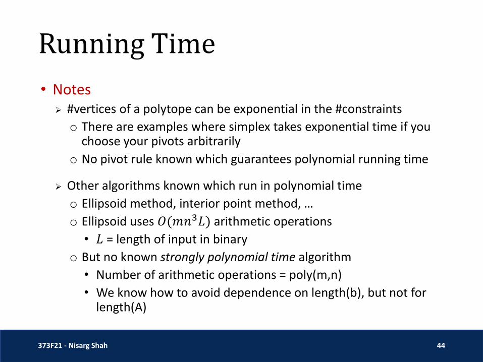
• Notes➢ #vertices of a polytope can be exponential in the #constraints
o There are examples where simplex takes exponential time if you choose your pivots arbitrarily
o No pivot rule known which guarantees polynomial running time
➢ Other algorithms known which run in polynomial time
o Ellipsoid method, interior point method, …
o Ellipsoid uses 𝑂(𝑚𝑛3𝐿) arithmetic operations
• 𝐿 = length of input in binary
o But no known strongly polynomial time algorithm
• Number of arithmetic operations = poly(m,n)
• We know how to avoid dependence on length(b), but not for length(A)

Certificate of Optimality
373F21 - Nisarg Shah 45
• Suppose you design a state-of-the-art LP solver that can solve very large problem instances
• You want to convince someone that you have this new technology without showing them the code➢ Idea: They can give you very large LPs and you can quickly return the
optimal solutions
➢ Question: But how would they know that your solutions are optimal, if they don’t have the technology to solve those LPs?

Certificate of Optimality
373F21 - Nisarg Shah 46
• Suppose I tell you that 𝑥1, 𝑥2 = (100,300) is optimal with objective value 1900
• How can you check this?➢ Note: Can easily substitute (𝑥1, 𝑥2), and verify that it is feasible, and
its objective value is indeed 1900

Certificate of Optimality
373F21 - Nisarg Shah 47
• Any solution that satisfies these inequalities also satisfies their positive combinations➢ E.g. 2*first_constraint + 5*second_constraint + 3*third_constraint
➢ Try to take combinations which give you 𝑥1 + 6𝑥2 on LHS
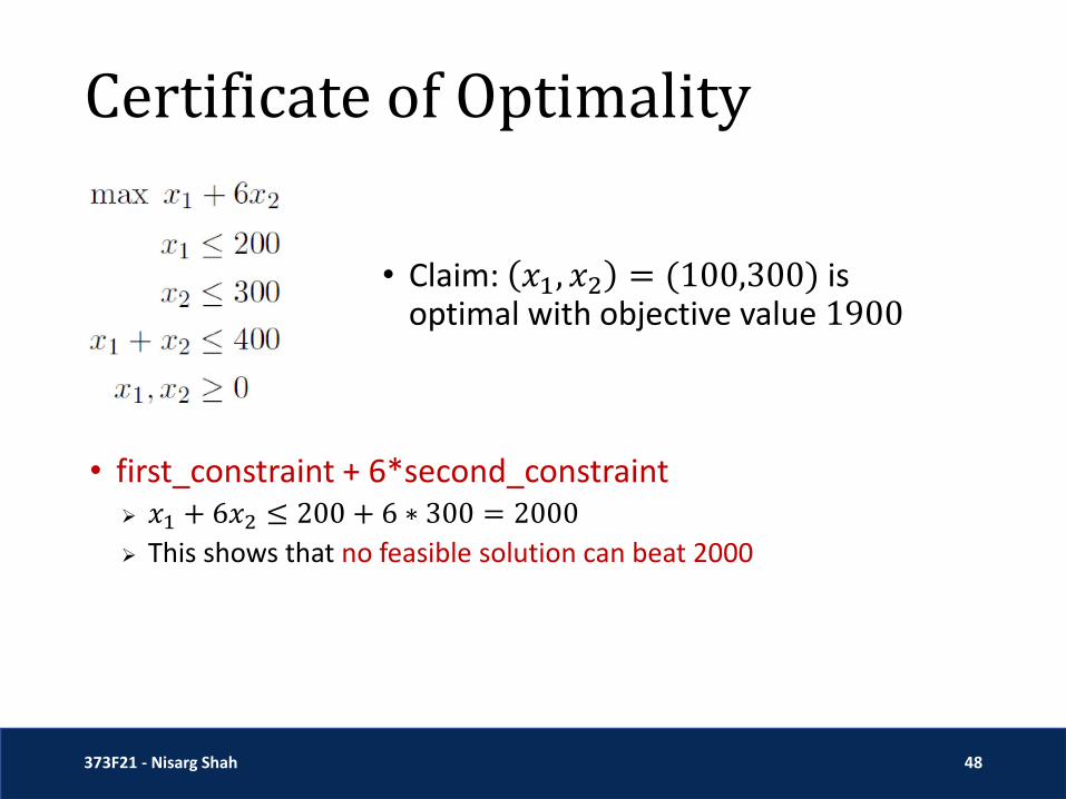
• Claim: 𝑥1, 𝑥2 = (100,300) is optimal with objective value 1900
Certificate of Optimality
373F21 - Nisarg Shah 48
• first_constraint + 6*second_constraint➢ 𝑥1 + 6𝑥2 ≤ 200 + 6 ∗ 300 = 2000
➢ This shows that no feasible solution can beat 2000
• Claim: 𝑥1, 𝑥2 = (100,300) is optimal with objective value 1900
Certificate of Optimality
373F21 - Nisarg Shah 49
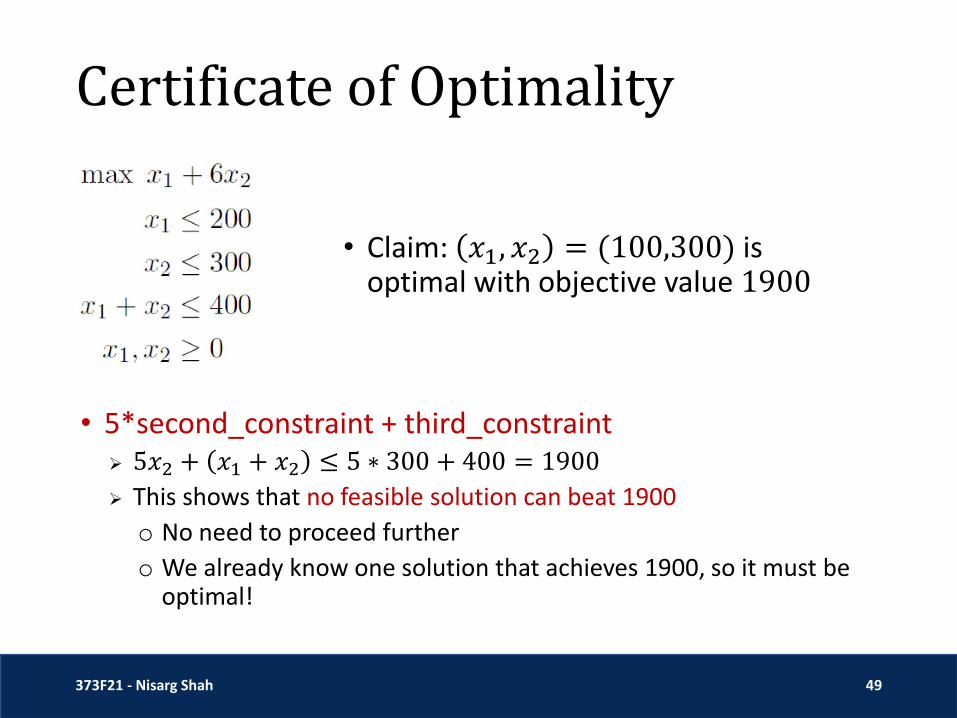
• 5*second_constraint + third_constraint➢ 5𝑥2 + 𝑥1 + 𝑥2 ≤ 5 ∗ 300 + 400 = 1900
➢ This shows that no feasible solution can beat 1900
o No need to proceed further
o We already know one solution that achieves 1900, so it must be optimal!
• Claim: 𝑥1, 𝑥2 = (100,300) is optimal with objective value 1900

Is There a General Algorithm?
373F21 - Nisarg Shah 50
• Introduce variables 𝑦1, 𝑦2, 𝑦3 by which we will be multiplying the three constraints➢ Note: These need not be integers. They can be reals.
• After multiplying and adding constraints, we get:𝑦1 + 𝑦3 𝑥1 + 𝑦2 + 𝑦3 𝑥2 ≤ 200𝑦1 + 300𝑦2 + 400𝑦3
Is There a General Algorithm?
373F21 - Nisarg Shah 51
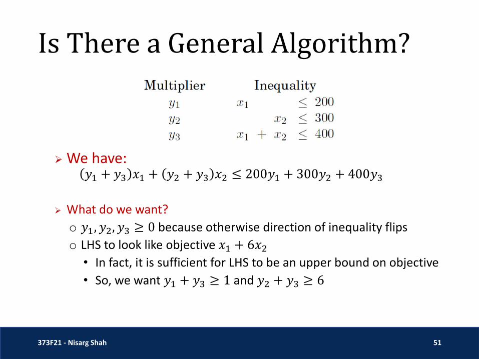
➢ We have: 𝑦1 + 𝑦3 𝑥1 + 𝑦2 + 𝑦3 𝑥2 ≤ 200𝑦1 + 300𝑦2 + 400𝑦3
➢ What do we want?
o 𝑦1, 𝑦2, 𝑦3 ≥ 0 because otherwise direction of inequality flips
o LHS to look like objective 𝑥1 + 6𝑥2• In fact, it is sufficient for LHS to be an upper bound on objective
• So, we want 𝑦1 + 𝑦3 ≥ 1 and 𝑦2 + 𝑦3 ≥ 6

Is There a General Algorithm?
373F21 - Nisarg Shah 52
➢ We have: 𝑦1 + 𝑦3 𝑥1 + 𝑦2 + 𝑦3 𝑥2 ≤ 200𝑦1 + 300𝑦2 + 400𝑦3
➢ What do we want?
o 𝑦1, 𝑦2, 𝑦3 ≥ 0
o 𝑦1 + 𝑦3 ≥ 1, 𝑦2 + 𝑦3 ≥ 6
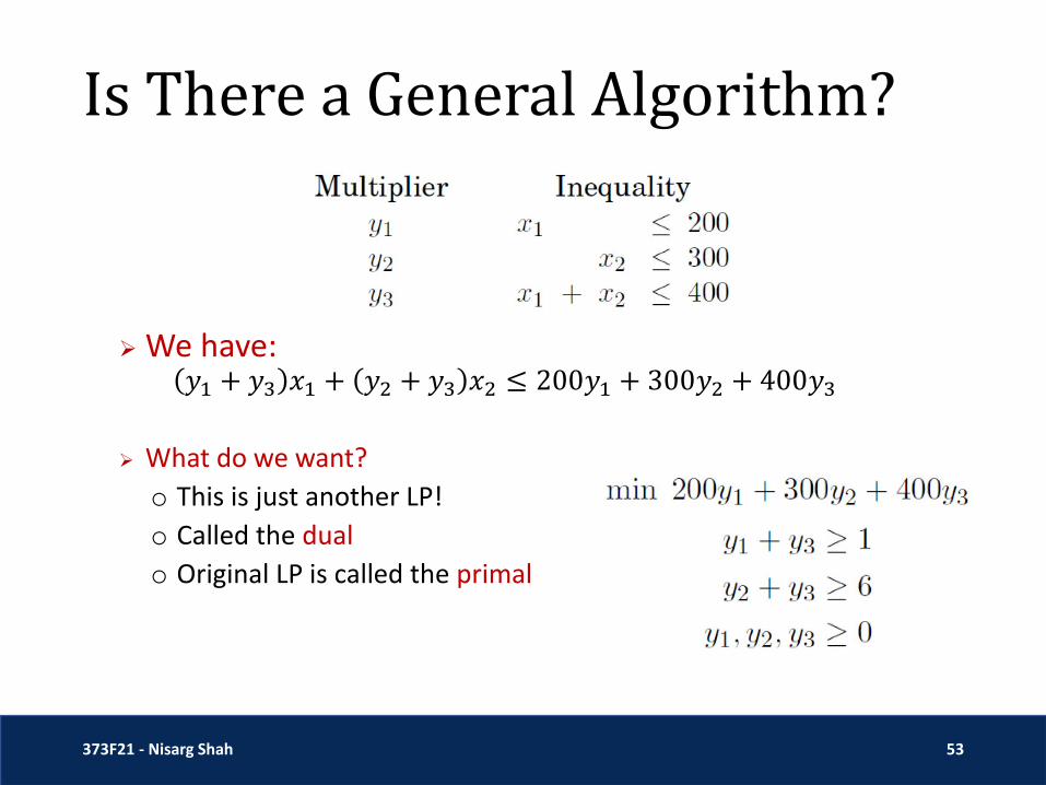
o Subject to these, we want to minimize the upper bound 200𝑦1 +300𝑦2 + 400𝑦3
Is There a General Algorithm?
373F21 - Nisarg Shah 53
➢ We have: 𝑦1 + 𝑦3 𝑥1 + 𝑦2 + 𝑦3 𝑥2 ≤ 200𝑦1 + 300𝑦2 + 400𝑦3
➢ What do we want?
o This is just another LP!
o Called the dual
o Original LP is called the primal

Is There a General Algorithm?
373F21 - Nisarg Shah 54
➢ The problem of verifying optimality is another LPo For any 𝑦1, 𝑦2, 𝑦3 that you can find, the objective value of the
dual is an upper bound on the objective value of the primal
o If you found a specific 𝑦1, 𝑦2, 𝑦3 for which this dual objective becomes equal to the primal objective for the (𝑥1, 𝑥2) given to you, then you would know that the given 𝑥1, 𝑥2 is optimal for primal (and your (𝑦1, 𝑦2, 𝑦3) is optimal for dual)

Is There a General Algorithm?
373F21 - Nisarg Shah 55
➢ The problem of verifying optimality is another LPo Issue 1: But…but…if I can’t solve large LPs, how will I solve the dual
to verify if optimality of (𝑥1, 𝑥2) given to me?
• You don’t. Ask the other party to give you both (𝑥1, 𝑥2) and the corresponding 𝑦1, 𝑦2, 𝑦3 for proof of optimality
o Issue 2: What if there are no (𝑦1, 𝑦2, 𝑦3) for which dual objective matches primal objective under optimal solution (𝑥1, 𝑥2)?
• As we will see, this can’t happen!

Is There a General Algorithm?
373F21 - Nisarg Shah 56
Primal LP Dual LP
➢ General version, in our standard form for LPs

Is There a General Algorithm?
373F21 - Nisarg Shah 57
Primal LP Dual LP
o 𝑐𝑇𝑥 for any feasible 𝑥 ≤ 𝑦𝑇𝑏 for any feasible 𝑦
o maxprimal feasible 𝑥
𝑐𝑇𝑥 ≤ mindual feasible 𝑦
𝑦𝑇𝑏
o If there is (𝑥∗, 𝑦∗) with 𝑐𝑇𝑥∗ = 𝑦∗ 𝑇𝑏, then both must be optimal
o In fact, for optimal 𝑥∗, 𝑦∗ , we claim that this must happen!
• Does this remind you of something? Max-flow, min-cut…

Weak Duality
373F21 - Nisarg Shah 58
• From here on, assume primal LP is feasible and bounded
• Weak duality theorem:➢ For any primal feasible 𝑥 and dual feasible 𝑦, 𝑐𝑇𝑥 ≤ 𝑦𝑇𝑏
• Proof:𝑐𝑇𝑥 ≤ 𝑦𝑇𝐴 𝑥 = 𝑦𝑇 𝐴𝑥 ≤ 𝑦𝑇𝑏
Primal LP Dual LP

Strong Duality
373F21 - Nisarg Shah 59
• Strong duality theorem:➢ For any primal optimal 𝑥∗ and dual optimal 𝑦∗, 𝑐𝑇𝑥∗ = 𝑦∗ 𝑇𝑏
Primal LP Dual LP
Strong Duality Proof
373F21 - Nisarg Shah 60
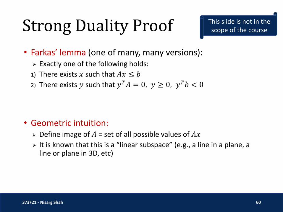
• Farkas’ lemma (one of many, many versions):➢ Exactly one of the following holds:
1) There exists 𝑥 such that 𝐴𝑥 ≤ 𝑏
2) There exists 𝑦 such that 𝑦𝑇𝐴 = 0, 𝑦 ≥ 0, 𝑦𝑇𝑏 < 0
• Geometric intuition:➢ Define image of 𝐴 = set of all possible values of 𝐴𝑥
➢ It is known that this is a “linear subspace” (e.g., a line in a plane, a line or plane in 3D, etc)
This slide is not in the scope of the course

Strong Duality Proof
373F21 - Nisarg Shah 61
• Farkas’ lemma: Exactly one of the following holds:1) There exists 𝑥 such that 𝐴𝑥 ≤ 𝑏
2) There exists 𝑦 such that 𝑦𝑇𝐴 = 0, 𝑦 ≥ 0, 𝑦𝑇𝑏 < 0
1) Image of 𝐴 contains a point “below” 𝑏 2) The region “below” 𝑏 doesn’t intersect image of 𝐴this is witnessed by normal vector to the image of 𝐴
This slide is not in the scope of the course

Strong Duality
373F21 - Nisarg Shah 62
• Strong duality theorem:➢ For any primal optimal 𝑥∗ and dual optimal 𝑦∗, 𝑐𝑇𝑥∗ = 𝑦∗ 𝑇𝑏
➢ Proof (by contradiction):
o Let 𝑧∗ = 𝑐𝑇𝑥∗ be the optimal primal value.
o Suppose optimal dual objective value > 𝑧∗
o So, there is no 𝑦 such that 𝑦𝑇𝐴 ≥ 𝑐𝑇 and 𝑦𝑇𝑏 ≤ 𝑧∗, i.e.,
Primal LP Dual LP
This slide is not in the scope of the course
Strong Duality
373F21 - Nisarg Shah 63
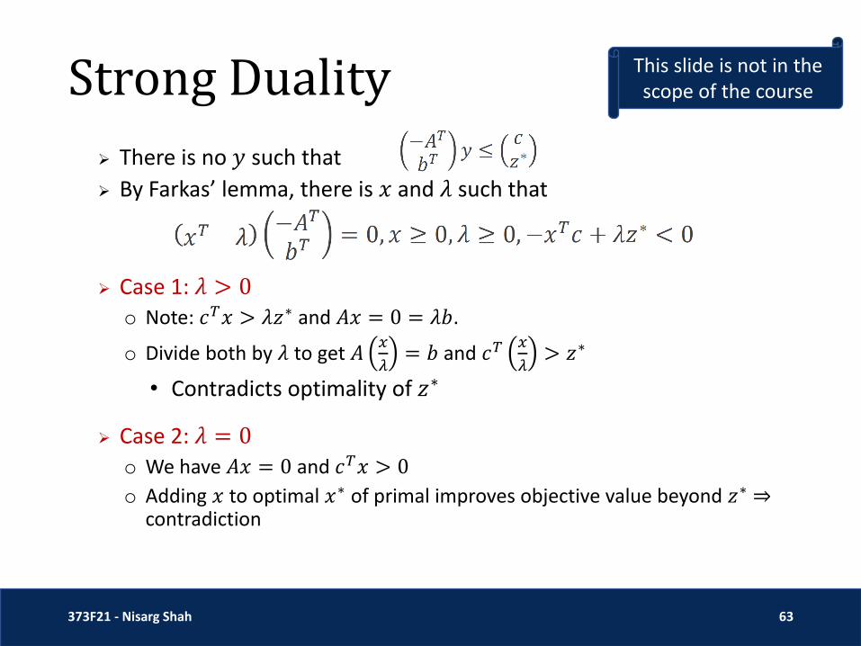
➢ There is no 𝑦 such that
➢ By Farkas’ lemma, there is 𝑥 and 𝜆 such that
➢ Case 1: 𝜆 > 0o Note: 𝑐𝑇𝑥 > 𝜆𝑧∗ and 𝐴𝑥 = 0 = 𝜆𝑏.
o Divide both by 𝜆 to get 𝐴𝑥
𝜆= 𝑏 and 𝑐𝑇
𝑥
𝜆> 𝑧∗
• Contradicts optimality of 𝑧∗
➢ Case 2: 𝜆 = 0
o We have 𝐴𝑥 = 0 and 𝑐𝑇𝑥 > 0
o Adding 𝑥 to optimal 𝑥∗ of primal improves objective value beyond 𝑧∗ ⇒contradiction
This slide is not in the scope of the course
Exercise: Formulating LPs
373F21 - Nisarg Shah 64
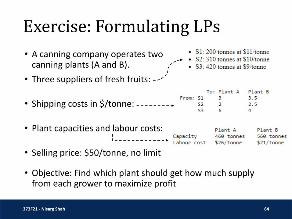
• A canning company operates twocanning plants (A and B).
• Three suppliers of fresh fruits:
• Shipping costs in $/tonne:
• Plant capacities and labour costs:
• Selling price: $50/tonne, no limit
• Objective: Find which plant should get how much supply from each grower to maximize profit
Exercise: Formulating LPs
373F21 - Nisarg Shah 66
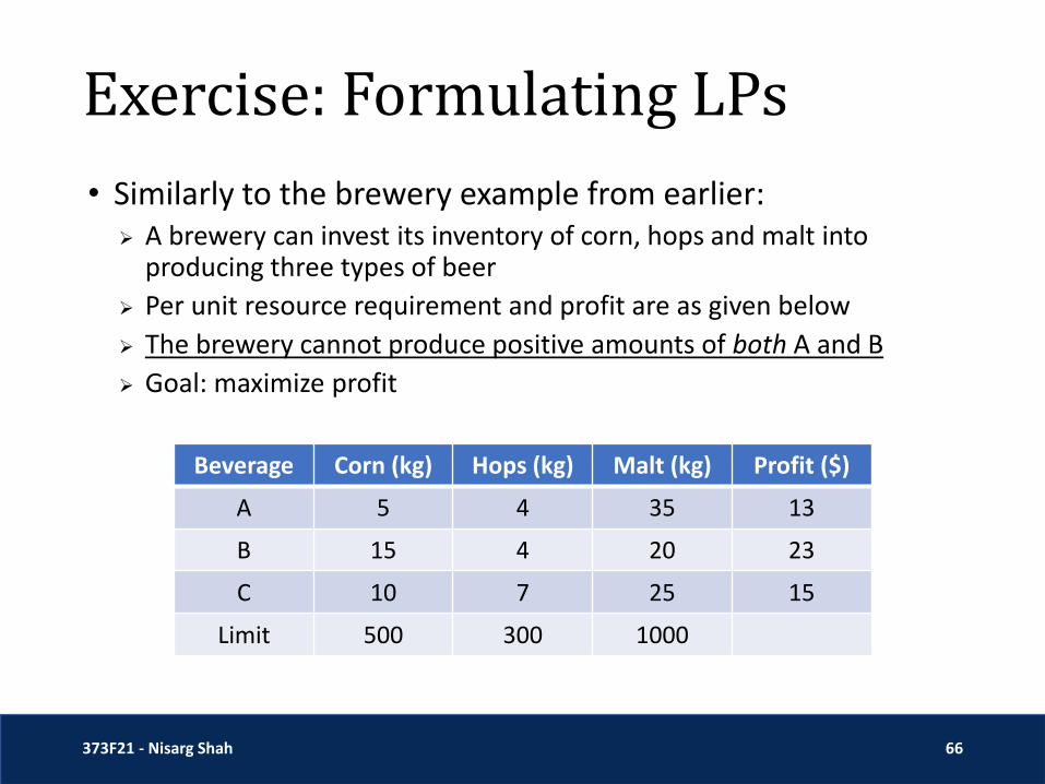
• Similarly to the brewery example from earlier:➢ A brewery can invest its inventory of corn, hops and malt into
producing three types of beer
➢ Per unit resource requirement and profit are as given below
➢ The brewery cannot produce positive amounts of both A and B
➢ Goal: maximize profit
Beverage Corn (kg) Hops (kg) Malt (kg) Profit ($)
A 5 4 35 13
B 15 4 20 23
C 10 7 25 15
Limit 500 300 1000

Exercise: Formulating LPs
373F21 - Nisarg Shah 67
• Similarly to the brewery example from the beginning:➢ A brewery can invest its inventory of corn, hops and malt into
producing three types of beer
➢ Per unit resource requirement and profit are as given below
➢ The brewery can only produce 𝐶 in integral quantities up to 100
➢ Goal: maximize profit
Beverage Corn (kg) Hops (kg) Malt (kg) Profit ($)
A 5 4 35 13
B 15 4 20 23
C 10 7 25 15
Limit 500 300 1000

Exercise: Formulating LPs
373F21 - Nisarg Shah 68
• Similarly to the brewery example from the beginning:➢ A brewery can invest its inventory of corn, hops and malt into
producing three types of beer
➢ Per unit resource requirement and profit are as given below
➢ Goal: maximize profit, but if there are multiple profit-maximizing solutions, then…
o Break ties to choose those with the largest quantity of 𝐴
o Break any further ties to choose those with the largest quantity of 𝐵
Beverage Corn (kg) Hops (kg) Malt (kg) Profit ($)
A 5 4 35 13
B 15 4 20 23
C 10 7 25 15
Limit 500 300 1000
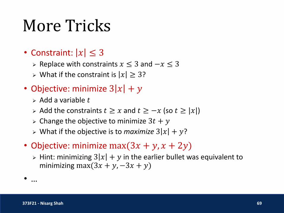
More Tricks
373F21 - Nisarg Shah 69
• Constraint: 𝑥 ≤ 3➢ Replace with constraints 𝑥 ≤ 3 and −𝑥 ≤ 3
➢ What if the constraint is 𝑥 ≥ 3?
• Objective: minimize 3 𝑥 + 𝑦➢ Add a variable 𝑡
➢ Add the constraints 𝑡 ≥ 𝑥 and 𝑡 ≥ −𝑥 (so 𝑡 ≥ |𝑥|)
➢ Change the objective to minimize 3𝑡 + 𝑦
➢ What if the objective is to maximize 3 𝑥 + 𝑦?
• Objective: minimize max(3𝑥 + 𝑦, 𝑥 + 2𝑦)➢ Hint: minimizing 3 𝑥 + 𝑦 in the earlier bullet was equivalent to
minimizing max(3𝑥 + 𝑦,−3𝑥 + 𝑦)
• …

373F21 - Nisarg Shah 70


