CSCI 1290: Comp Photo

Fall 2018 @ Brown UniversityJames Tompkin

Many slides thanks to James Hays’ old CS 129 course, along with all of its acknowledgements.

Alan hours today

• 16:00 – 18:00

• CIT 203

• HDR project code support

Image Compositing (Szeliski 9.3.4)

Google Street View

Many slides from Alexei Efros

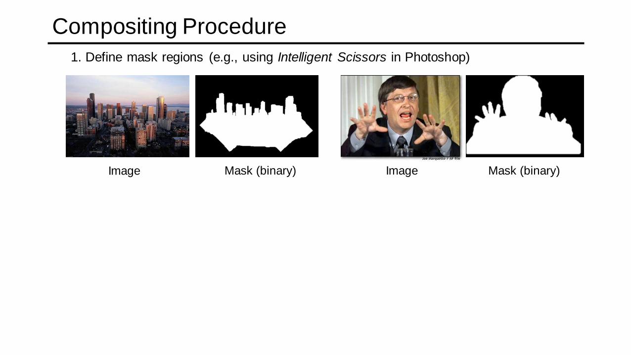
Compositing Procedure

1. Define mask regions (e.g., using Intelligent Scissors in Photoshop)

Image Mask (binary) Image Mask (binary)

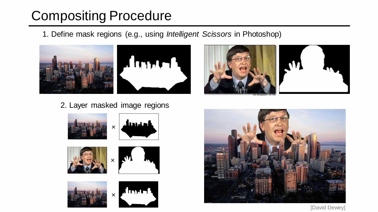
Compositing Procedure

1. Define mask regions (e.g., using Intelligent Scissors in Photoshop)

[David Dewey]

2. Layer masked image regions

×

×

×

Artifacts in simple masking

[David Dewey]

- Staircasing

- Fringing or

subtle halo

Goes back to one of our

motivating questions:

What is a pixel?

Masks are not enough.

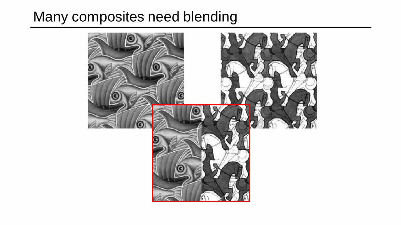
Many composites need blending

Alpha channel

Add one more channel:

• Image(R,G,B,alpha)

Encodes transparency (or pixel coverage):

• Alpha = 1: opaque object (complete coverage)

• Alpha = 0: transparent object (no coverage)

• 0<Alpha<1: semi-transparent (partial coverage)

Example: alpha = 0.7

Partial coverage or semi-transparency

Multiple Alpha Blending

So far we assumed that one image (background) is opaque.

If blending semi-transparent sprites (the “A over B”

operation):

Icomp = aaIa + (1-aa)abIb

acomp = aa + (1-aa)ab

Note: sometimes alpha is premultiplied:

im(aR,aG,aB,a):

Icomp = Ia + (1-aa)Ib(same for alpha!)

Alpha Blending / Feathering

01

01

+

= Iblend = aIleft + (1-a)Iright

× ×

Alpha

matte

Setting alpha: simple averaging

Alpha = .5 in overlap region

Setting alpha: center seam

Alpha = logical(dtrans1>dtrans2)

Distance

Transformbwdist

Setting alpha: blurred seam

Alpha = blurred

Distance

transform

Setting alpha: center weighting

Alpha = dtrans1 / (dtrans1+dtrans2)

Distance

transform

Ghost!

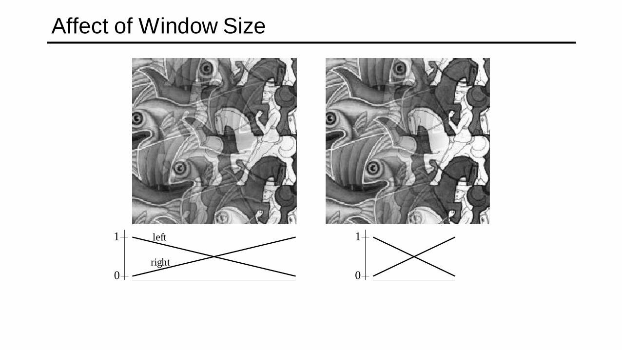
Affect of Window Size

0

1 left

right

0

1

Affect of Window Size

0

1

0

1

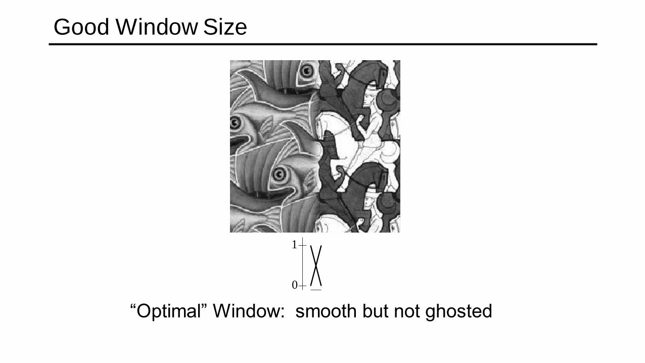
Good Window Size

0

1

“Optimal” Window: smooth but not ghosted

Laplacian (derivative of Gaussian) Pyramid

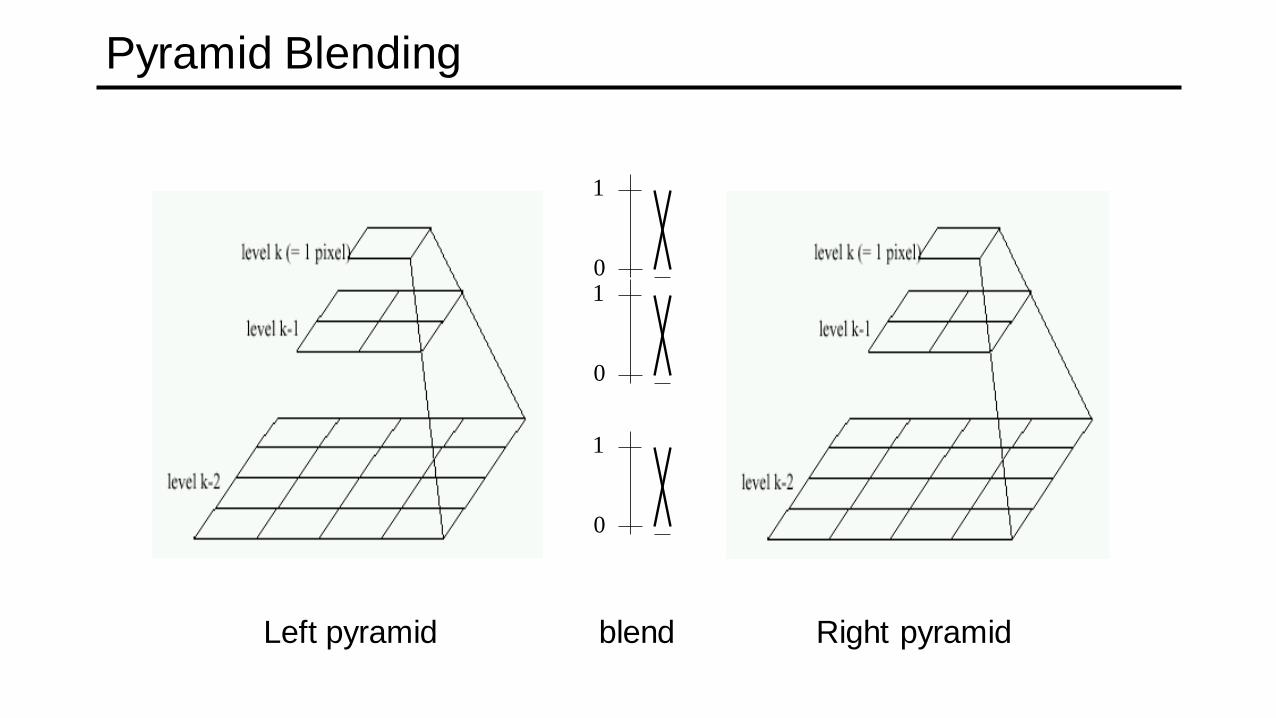
Pyramid Blending

0

1

0

1

0

1

Left pyramid Right pyramidblend

Pyramid Blending

laplacian

level

4

laplacian

level

2

laplacian

level

0

left pyramid right pyramid blended pyramid

Laplacian Pyramid: Blending

General Approach:1. Build Laplacian pyramids LA and LB from images A and B

2. Build a Gaussian pyramid GR from selected region R

3. Form a combined pyramid LS from LA and LB using nodes of GR as weights:

• LS(i,j) = GR(I,j,)*LA(I,j) + (1-GR(I,j))*LB(I,j)

4. Collapse the LS pyramid to get the final blended image

Blending Regions

Horror Photo

david dmartin (Boston College)

Chris Cameron

Simplification: Two-band Blending

Brown & Lowe, 2003• Only use two bands: high freq. and low freq.

• Blends low freq. smoothly

• Blend high freq. with no smoothing: use binary alpha

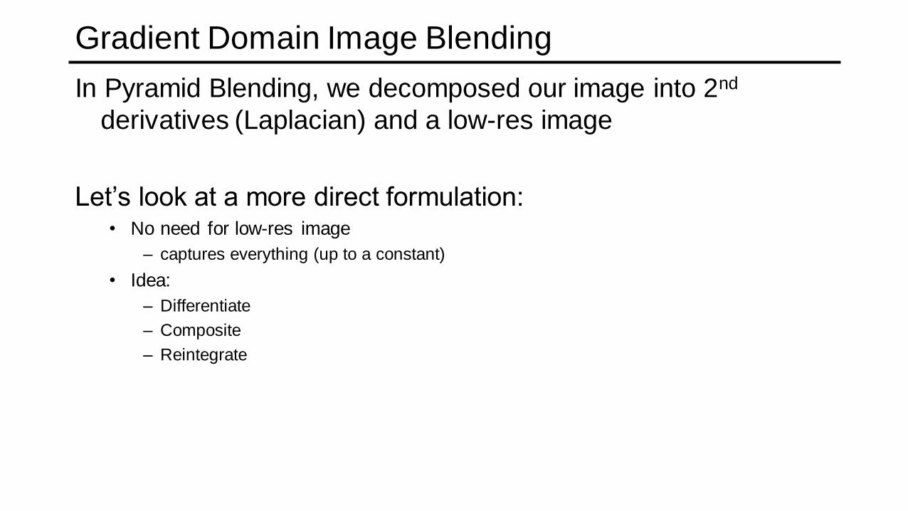
Gradient Domain Image Blending

In Pyramid Blending, we decomposed our image into 2nd

derivatives (Laplacian) and a low-res image

Let’s look at a more direct formulation:• No need for low-res image

– captures everything (up to a constant)

• Idea:

– Differentiate

– Composite

– Reintegrate

Gradient Domain blending (1D)

Two

signals

Regular

blendingBlending

derivatives

bright

dark

Gradient Domain Blending (2D)

Trickier in 2D:• Take partial derivatives dx and dy (the gradient field)

• Manipulate them (smooth, blend, feather, etc. as needed)

• Reintegrate

– But now integral(dx) might not equal integral(dy)

• Find the most agreeable solution

– Equivalent to solving Poisson equation (partial differential equation)

– Can use FFT, deconvolution, multigrid solvers, etc.

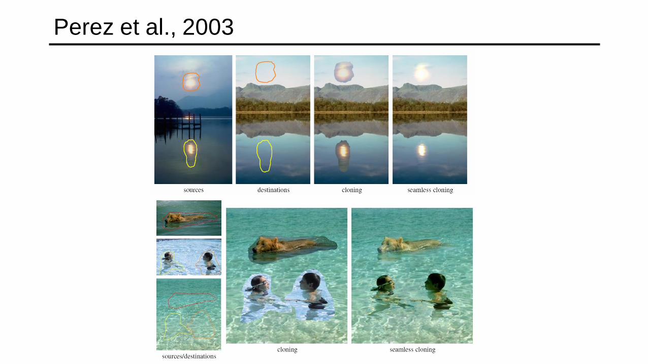
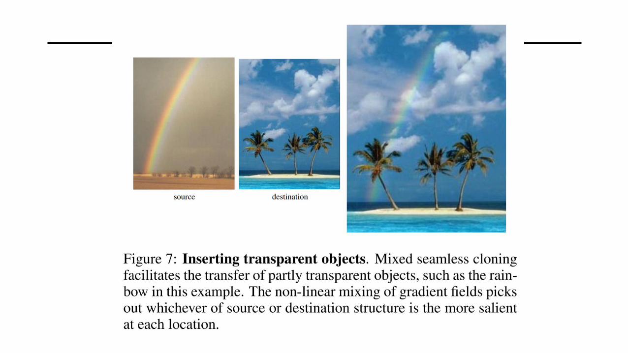
Perez et al., 2003

Perez et al., 2003

Limitations:• Can’t negate gradients, e.g., contrast reversal (gray on black -> gray on white)

• Colored backgrounds “bleed through”

• Images need to be very well aligned

Editing

Gradient Domain Blending

[James Hays]

Project details not shown in class

sourcetarget

It is impossible to faithfully preserve the gradients

sourcetarget

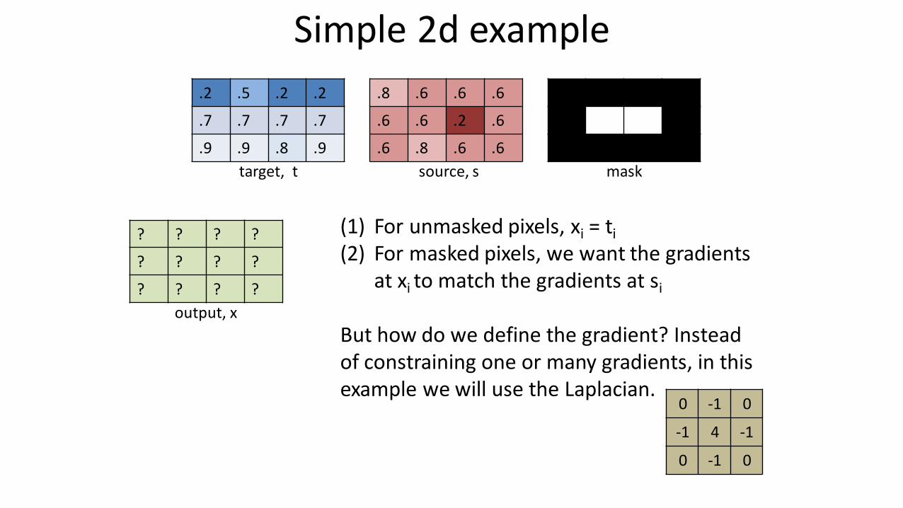
Simple 2d example

source, starget, t mask

.2 .5 .2 .2

.7 .7 .7 .7

.9 .9 .8 .9

.8 .6 .6 .6

.6 .6 .2 .6

.6 .8 .6 .6

output, x

? ? ? ?

? ? ? ?

? ? ? ?

What properties do we want x to have?

Simple 2d example

source, starget, t mask

.8 .6 .6 .6

.6 .6 .2 .6

.6 .8 .6 .6

.2 .5 .2 .2

.7 .7 .7 .7

.9 .9 .8 .9

(1) For unmasked pixels, xi = ti

(2) For masked pixels, we want the gradients at xi to match the gradients at si

But how do we define the gradient? Instead of constraining one or many gradients, in this example we will use the Laplacian.

output, x

? ? ? ?

? ? ? ?

? ? ? ?

0 -1 0

-1 4 -1

0 -1 0

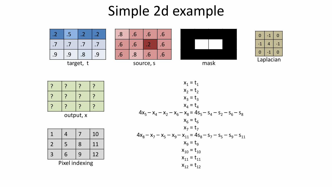
Simple 2d example

source, starget, t mask

.8 .6 .6 .6

.6 .6 .2 .6

.6 .8 .6 .6

Pixel indexing

1 4 7 10

2 5 8 11

3 6 9 12

output, x

? ? ? ?

? ? ? ?

? ? ? ?

x1 = t1

x2 = t2

x3 = t3

x4 = t4

4x5 – x4 – x2 – x6 – x8 = 4s5 – s4 – s2 – s6 – s8

x6 = t6

x7 = t7

4x8 – x7 – x5 – x9 – x11 = 4s8 – s7 – s5 – s9 – s11

x9 = t9

x10 = t10

x11 = t11

x12 = t12

.2 .5 .2 .2

.7 .7 .7 .7

.9 .9 .8 .9

0 -1 0

-1 4 -1

0 -1 0

Laplacian

Simple 2d example

source, starget, t mask

.8 .6 .6 .6

.6 .6 .2 .6

.6 .8 .6 .6

Pixel indexing

1 4 7 10

2 5 8 11

3 6 9 12

output, x

? ? ? ?

? ? ? ?

? ? ? ?

x1 = 0.2x2 = 0.7x3 = 0.9x4 = 0.5

4x5 – x4 – x2 – x6 – x8 = 0.2x6 = 0.9x7 = 0.2

4x8 – x7 – x5 – x9 – x11 = -1.6x9 = 0.8

x10 = 0.2x11 = 0.7x12 = 0.9

.2 .5 .2 .2

.7 .7 .7 .7

.9 .9 .8 .9

0 -1 0

-1 4 -1

0 -1 0

Laplacian

* =

Simple 2d example

source, starget, t mask

.8 .6 .6 .6

.6 .6 .2 .6

.6 .8 .6 .6

Pixel indexing

1 4 7 10

2 5 8 11

3 6 9 12

output, x

? ? ? ?

? ? ? ?

? ? ? ?

.2 .5 .2 .2

.7 .7 .7 .7

.9 .9 .8 .9

0 -1 0

-1 4 -1

0 -1 0

Laplacian

1

1

1

1

-1 -1 4 -1 -1

1

1

-1 -1 4 -1 -1

1

1

1

1

.2

.7

.9

.5

.2

.9

.2

-1.6

.8

.2

.7

.9

A x b

?

?

?

?

?

?

?

?

?

?

?

?

x = A\b

* =

Simple 2d example

source, starget, t mask

.8 .6 .6 .6

.6 .6 .2 .6

.6 .8 .6 .6

Pixel indexing

1 4 7 10

2 5 8 11

3 6 9 12

output, x

? ? ? ?

? ? ? ?

? ? ? ?

.2 .5 .2 .2

.7 .7 .7 .7

.9 .9 .8 .9

0 -1 0

-1 4 -1

0 -1 0

Laplacian

1

1

1

1

-1 -1 4 -1 -1

1

1

-1 -1 4 -1 -1

1

1

1

1

.2

.7

.9

.5

.62

.9

.2

.18

.8

.2

.7

.9

.2

.7

.9

.5

.2

.9

.2

-1.6

.8

.2

.7

.9

A x b

output = reshape(x, 3, 4).2 .5 .2 .2

.7 .62 .18 .7

.9 .9 .8 .9

sourcetarget mask

no blending gradient domain blending

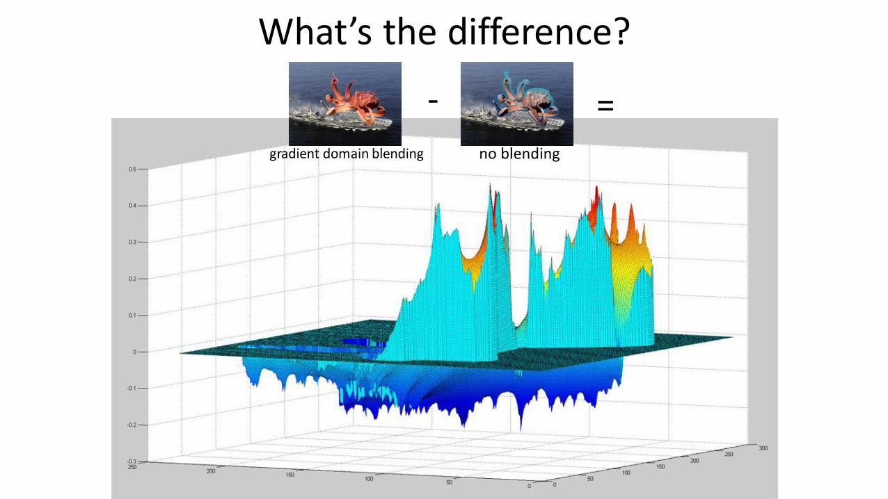
What’s the difference?

no blendinggradient domain blending

- =

What’s the difference?

no blendinggradient domain blending

- =

What’s the difference?

no blendinggradient domain blending

- =

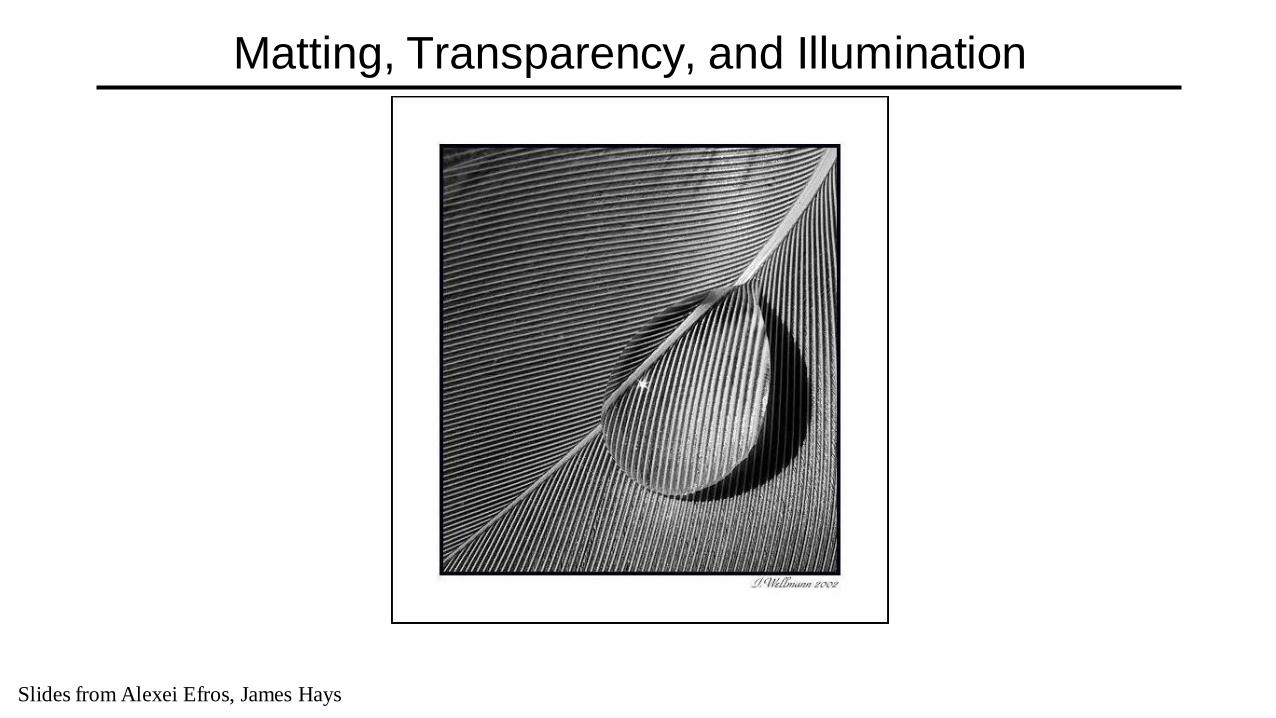
Matting, Transparency, and Illumination

Slides from Alexei Efros, James Hays

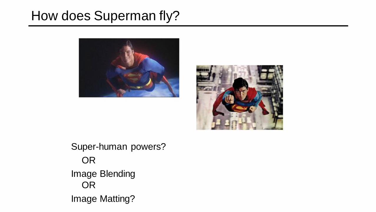
How does Superman fly?

Super-human powers?

OR

Image Blending

OR

Image Matting?

Physics of Alpha Matting

Semi-transparent objects

Pixels too large to capture surface

“Pulling a Matte”

Problem Definition:

• The separation of an image C into

– A foreground object image Co,

– a background image Cb,

– and an alpha matte a

• Co and a can then be used to composite the foreground

object into a different image

Hard problem

• Even if alpha is binary, this is hard to do automatically

(background subtraction problem)

• For movies/TV, manual segmentation of each frame is

difficult

• Need to make a simplifying assumption…

Average/Median Image

What can we do with this?

Background Subtraction

-

=

Background Subtraction

A largely unsolved problem…

Estimated

background

Difference

Image

Thresholded

Foreground

on blue

One video

frame

Blue Screen

Blue Screen matting

Most common form of matting in TV studios & movies

Petros Vlahos invented blue screen matting in the 50s.

His Ultimatte® is still the most popular equipment. He

won an Oscar for lifetime achievement.

A form of background subtraction:

• Need a known background

• Compute alpha as SSD(C,Cb) > threshold

– Or use Vlahos’ formula: a = 1-p1(B-p2G)

• Hope that foreground object doesn’t look like background

– no blue ties!

• Why blue?

• Why uniform?

The Ultimatte

p1 and p2

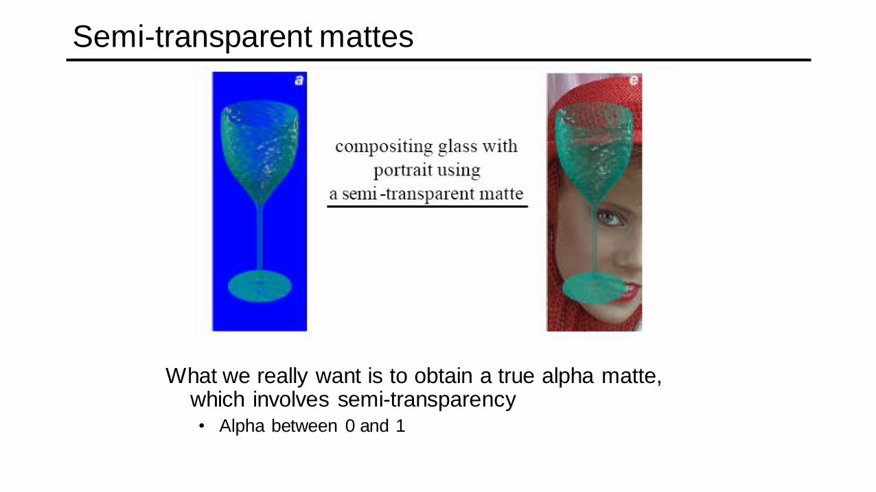
Semi-transparent mattes

What we really want is to obtain a true alpha matte, which involves semi-transparency• Alpha between 0 and 1

Matting Problem: Mathematical Definition

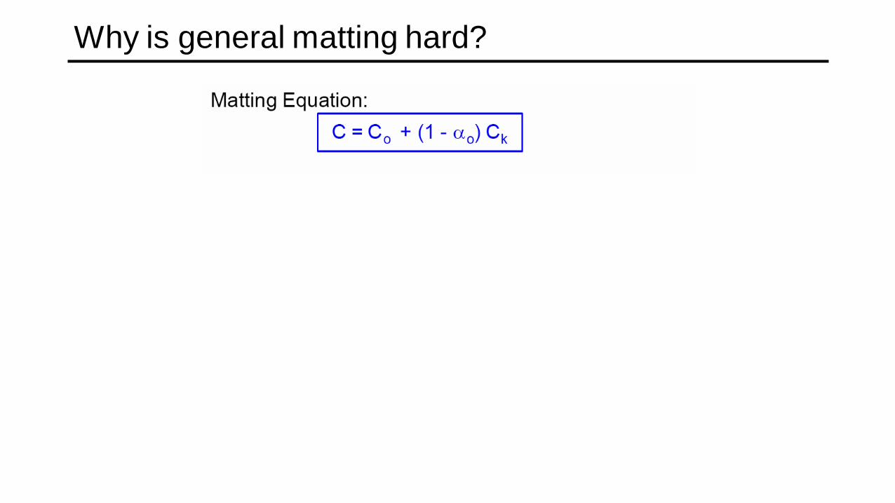
Why is general matting hard?

Solution #1: No Blue!

Solution #2: Gray or Flesh

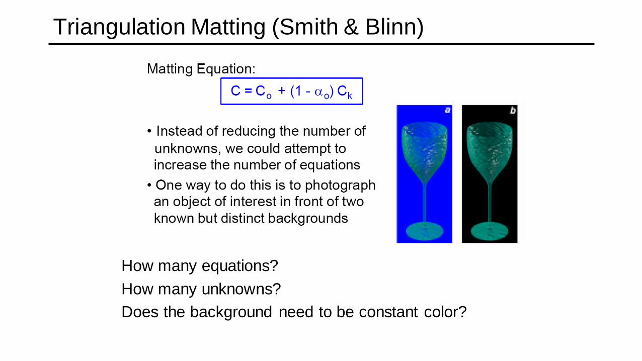
Triangulation Matting (Smith & Blinn)

How many equations?

How many unknowns?

Does the background need to be constant color?

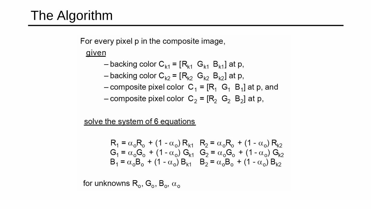
The Algorithm

Triangulation Matting Examples

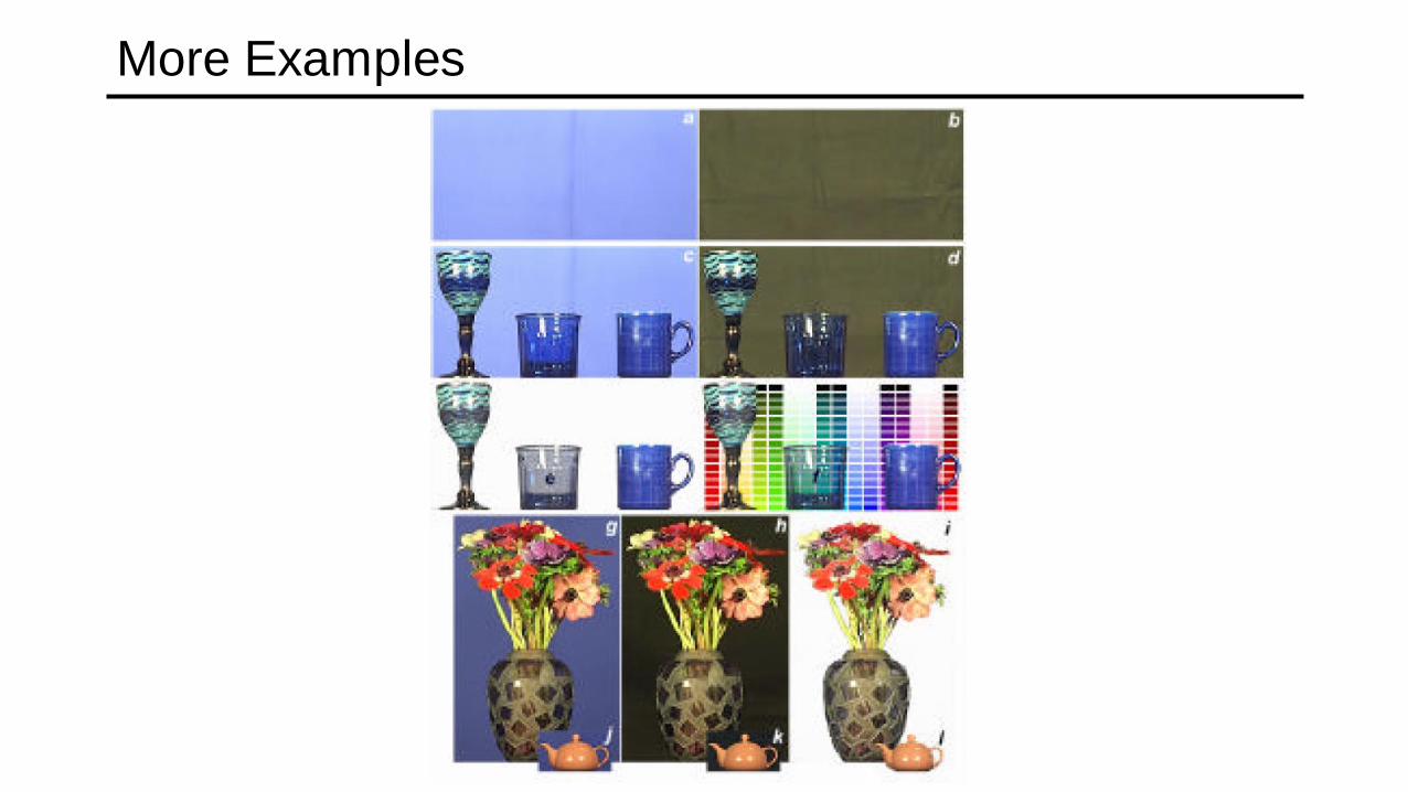
More Examples

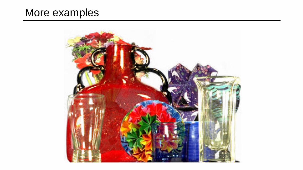
More examples

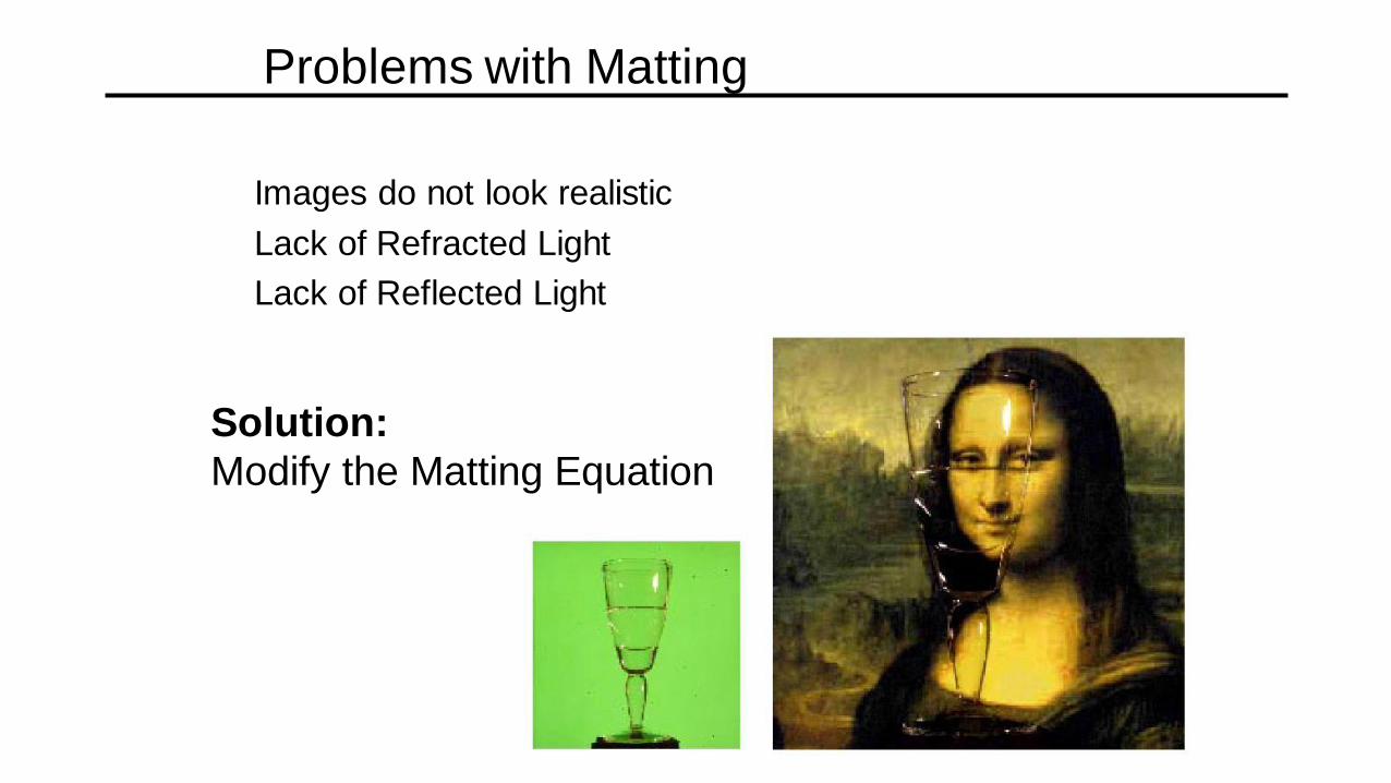
Problems with Matting

Images do not look realistic

Lack of Refracted Light

Lack of Reflected Light

Solution:

Modify the Matting Equation

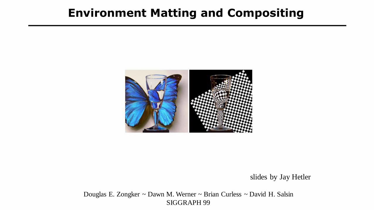
Environment Matting and Compositing

slides by Jay Hetler

Douglas E. Zongker ~ Dawn M. Werner ~ Brian Curless ~ David H. Salsin

SIGGRAPH 99

Environment Matting Equation

C = F + (1- a)B + F

C ~ Color

F ~ Foreground color

B ~ Background color

a ~ Amount of light that passes through the foreground

F ~ Contribution of light from Environment that travels through the object

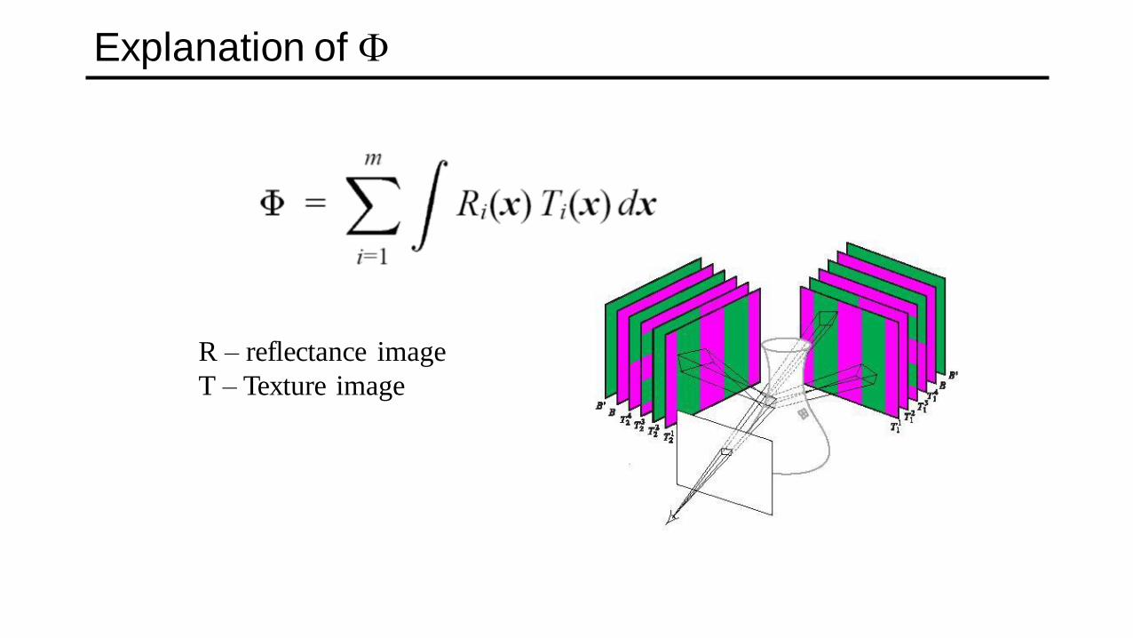
Explanation of F

R – reflectance image

T – Texture image

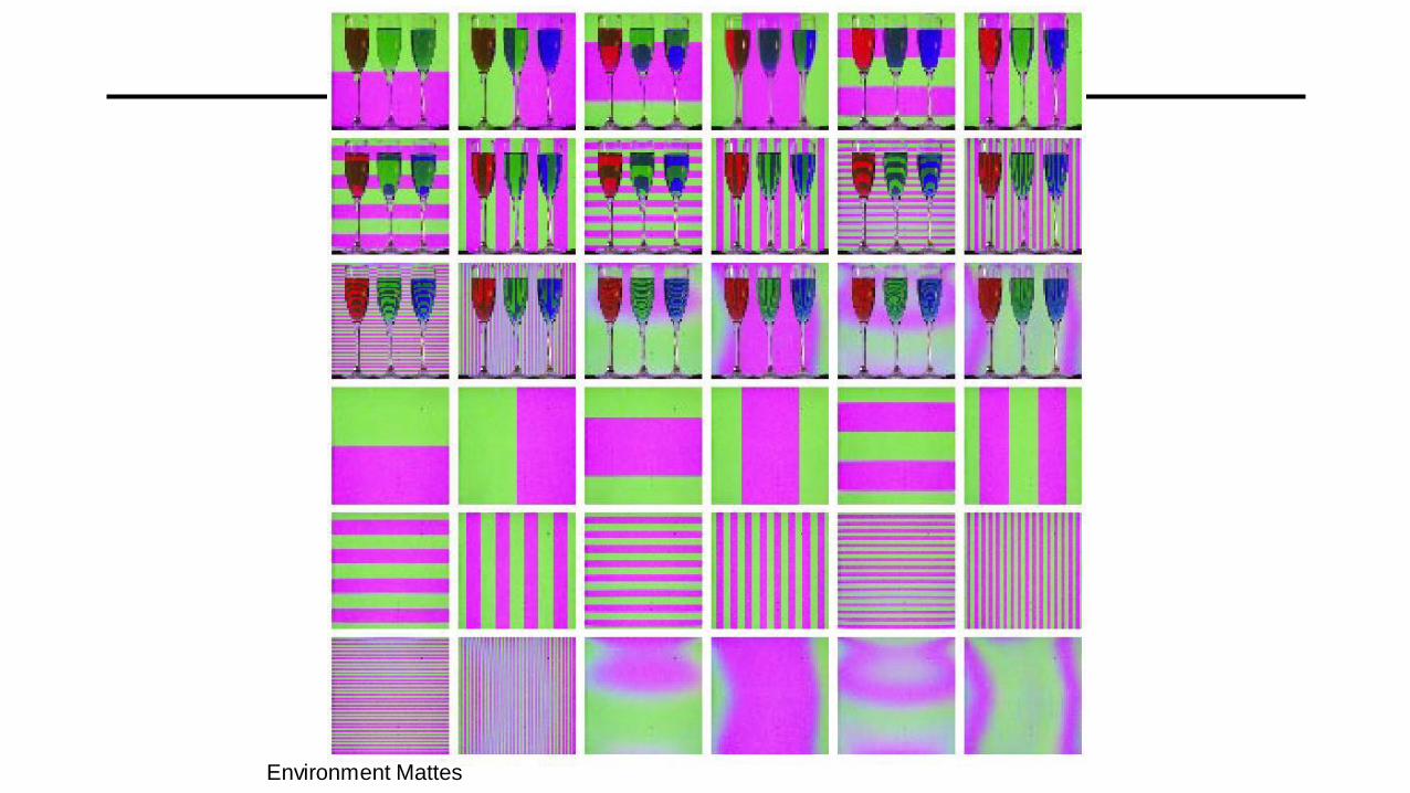
Environment Mattes

How much better is Environment Matting?

Alpha Matte Environment Matte Photograph

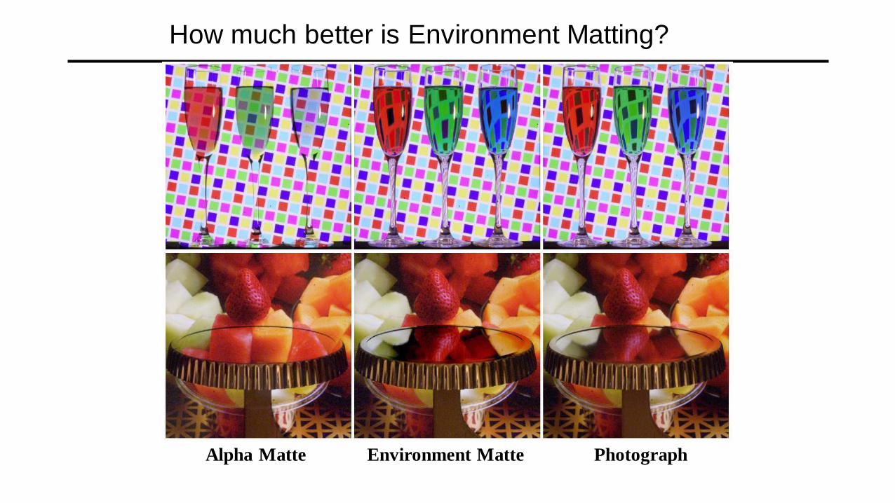
How much better is Environment Matting?

Alpha Matte Environment Matte Photograph