71
CSE 245: Computer Aided Circuit Simulation and Verification Fall 2004, Oct 19 Lecture 7: Matrix Solver II -Iterative Method
| Date post: | 31-Dec-2015 |
| Category: |
Documents |
| Upload: | vaughan-moody |
| View: | 33 times |
| Download: | 0 times |

CSE 245: Computer Aided Circuit Simulation and Verification
Fall 2004, Oct 19
Lecture 7:
Matrix Solver II
-Iterative Method

April 19, 2023 Lecture 7.2 Zhengyong (Simon) Zhu, UCSD
Outline Iterative Method
Stationary Iterative Method (SOR, GS,Jacob) Krylov Method (CG, GMRES) Multigrid Method

April 19, 2023 Lecture 7.3 courtesy Alessandra Nardi, UCB
Iterative Methods
Stationary: x(k+1) =Gx(k)+cwhere G and c do not depend on iteration
count (k)
Non Stationary:x(k+1) =x(k)+akp(k)
where computation involves information that change at each iteration
April 19, 2023 Lecture 7.4 courtesy Alessandra Nardi, UCB
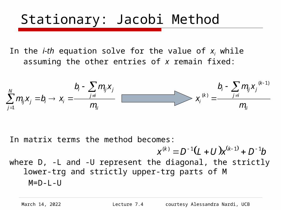
In the i-th equation solve for the value of xi while assuming the other entries of x remain fixed:
In matrix terms the method becomes:
where D, -L and -U represent the diagonal, the strictly lower-trg and strictly upper-trg parts of M
M=D-L-U
ii
ijjiji
i
N
jijij m
xmb
xbxm
1 ii
ij
kjiji
ki m
xmb
x
)1(
)(
bDxULDx kk 111)(
Stationary: Jacobi Method

April 19, 2023 Lecture 7.5 courtesy Alessandra Nardi, UCB
Like Jacobi, but now assume that previously computed results are used as soon as they are available:
In matrix terms the method becomes:
where D, -L and -U represent the diagonal, the strictly lower-trg and strictly upper-trg parts of M
M=D-L-U
ii
ijjiji
i
N
jijij m
xmb
xbxm
1 ii
ij
kjij
ij
kjiji
ki m
xmxmb
x
)1()(
)(
)( 11)( bUxLDx kk
Stationary-Gause-Seidel

April 19, 2023 Lecture 7.6 courtesy Alessandra Nardi, UCB
Devised by extrapolation applied to Gauss-Seidel in the form of weighted average:
In matrix terms the method becomes:
where D, -L and -U represent the diagonal, the strictly lower-trg and strictly upper-trg parts of M
M=D-L-U
ii
ij
kjij
ij
kjiji
ki m
xmxmb
x
)1()(
)(
bwLDwxDwwUwLDx kk 111)( )())1((
)1()()( )1( ki
ki
ki xwxwx
Stationary: Successive Overrelaxation (SOR)

April 19, 2023 Lecture 7.7 Zhengyong (Simon) Zhu, UCSD
SOR Choose w to accelerate the convergence
W =1 : Jacobi / Gauss-Seidel 2>W>1: Over-Relaxation W < 1: Under-Relaxation
)1()()( )1( ki
ki
ki xwxwx

April 19, 2023 Lecture 7.8 Zhengyong (Simon) Zhu, UCSD
Convergence of Stationary Method Linear Equation: MX=b A sufficient condition for convergence of the
solution(GS,Jacob) is that the matrix M is diagonally dominant.
If M is symmetric positive definite, SOR converges for any w (0<w<2)
A necessary and sufficient condition for the convergence is the magnitude of the largest eigenvalue of the matrix G is smaller than 1
Jacobi: Gauss-Seidel SOR:
N
ijjjiii mm
&1,
ULDG 1
ULDG 1)(
))1((1 DwwUwLDG

April 19, 2023 Lecture 7.9 Zhengyong (Simon) Zhu, UCSD
Outline Iterative Method
Stationary Iterative Method (SOR, GS,Jacob) Krylov Method (CG, GMRES)
Steepest Descent Conjugate Gradient Preconditioning
Multigrid Method

April 19, 2023 Lecture 7.10 Zhengyong (Simon) Zhu, UCSD
Linear Equation: an optimization problem Quadratic function of vector x
Matrix A is positive-definite, if for any nonzero vector x
If A is symmetric, positive-definite, f(x) is minimized by the solution bAx
cxbAxxxf TT 21)(
0AxxT

April 19, 2023 Lecture 7.11 Zhengyong (Simon) Zhu, UCSD
Linear Equation: an optimization problem
Quadratic function
Derivative
If A is symmetric
If A is positive-definite is minimized by setting to 0
cxbAxxxf TT 21)(
bAxxAxf T 21
21)(
bAxxf )(
)(xf )(xf
bAx

April 19, 2023 Lecture 7.12 from J. R. Shewchuk "painless CG"
For symmetric positive definite matrix A

April 19, 2023 Lecture 7.13 from J. R. Shewchuk "painless CG"
Gradient of quadratic form
The points in the direction of steepest increase of f(x)

April 19, 2023 Lecture 7.14 Zhengyong (Simon) Zhu, UCSD
If A is symmetric positive definite P is the arbitrary point X is the solution point
Symmetric Positive-Definite Matrix A
bAx 1
)()()()( 21 xpAxpxfpf T
0)()(21 xpAxp T
since
)()( xfpf We have,
If p != x

April 19, 2023 Lecture 7.15 from J. R. Shewchuk "painless CG"
If A is not positive definite
a) Positive definite matrix b) negative-definite matrix c) Singular matrix d) positive indefinite matrix

April 19, 2023 Lecture 7.16 Zhengyong (Simon) Zhu, UCSD
Non-stationary Iterative Method State from initial guess x0, adjust it until
close enough to the exact solution
How to choose direction and step size?
)()()()1( iiii paxx i=0,1,2,3,……
)(ip
)(iaAdjustment Direction
Step Size

April 19, 2023 Lecture 7.17 Zhengyong (Simon) Zhu, UCSD
Steepest Descent Method (1)
)()()( )( iii rAxbxf
Choose the direction in which f decrease most quickly: the direction opposite of
Which is also the direction of residue
)( )(ixf
)()()()1( iiii raxx

April 19, 2023 Lecture 7.18 Zhengyong (Simon) Zhu, UCSD
Steepest Descent Method (2) How to choose step size ?
Line Search should minimize f, along the direction
of , which means 0)( )1( idad xf
0)()()( )()1()1()1()1( iT
iidadT
iidad rxfxxfxf
)()(
)()(
)(
)()()()()(
)()()()(
)()1(
)()1(
)()(
0))((
0)(
0
iT
i
iT
i
Arr
rr
i
iT
iiiT
i
iT
iii
iT
i
iT
i
a
rArarAxb
rraxAb
rAxb
rr
)(ir)(ia
Orthogonal

April 19, 2023 Lecture 7.19 Zhengyong (Simon) Zhu, UCSD
Steepest Descent Algorithm
)()()()1(
)(
)()(
)()(
)()(
iiii
Arr
rr
i
ii
raxx
a
Axbr
iT
i
iT
i
Given x0, iterate until residue is smaller than error tolerance

April 19, 2023 Lecture 7.20 from J. R. Shewchuk "painless CG"
Steepest Descent Method: example
8
2
62
23
2
1
x
x
a) Starting at (-2,-2) take thedirection of steepest descent of f
b) Find the point on the intersec-tion of these two surfaces that minimize f
c) Intersection of surfaces.
d) The gradient at the bottommostpoint is orthogonal to the gradientof the previous step

April 19, 2023 Lecture 7.21 from J. R. Shewchuk "painless CG"
Iterations of Steepest Descent Method

April 19, 2023 Lecture 7.22 Zhengyong (Simon) Zhu, UCSD
Convergence of Steepest Descent-1
k
v Tk ]0,0,0,,1,,0,0,0[ let
n
jjji ve
1)( Eigenvector:
2/1)( Aeee T
AEnergy norm:
EigenValue:j j=1,2,…,n

April 19, 2023 Lecture 7.23 Zhengyong (Simon) Zhu, UCSD
Convergence of Steepest Descent-2
))((
)(
1,
))((
)(
1))((
)(1
)()()(2
2
)()(
232
222
222
)(
232
222
2
)()()()()(
2)()(2
)(
)()(
2)()(2
)()()(2
)()(
)()()()(
)()(
)()(2
)(
)()(2
)()()()()()(
)()()()()()(
)1()1(
2
)1(
jjj
jjj
jjj
Ai
jjj
jjj
jjj
Aii
Tii
Ti
iTi
Ai
iTi
iTi
AiiTi
iTi
iTi
iTi
iTi
iTi
Ai
iTiii
Tiii
Ti
iiiTii
Ti
iTiAi
e
eAeeArr
rre
Arr
rreArr
Arr
rrrr
Arr
rre
ArraAeraAee
raeArae
Aeee

April 19, 2023 Lecture 7.24 Zhengyong (Simon) Zhu, UCSD
Convergence Study (n=2)
assume21
let21 /k Spectral condition number
2
1)(
jjji ve let 12 /u
))((
)(1
))((
)(1
232
222
32
22
31
212
221
21
222
22
21
212
ukuk
uk

April 19, 2023 Lecture 7.25 from J. R. Shewchuk "painless CG"
Plot of w

April 19, 2023 Lecture 7.26 from J. R. Shewchuk "painless CG"
Case Study
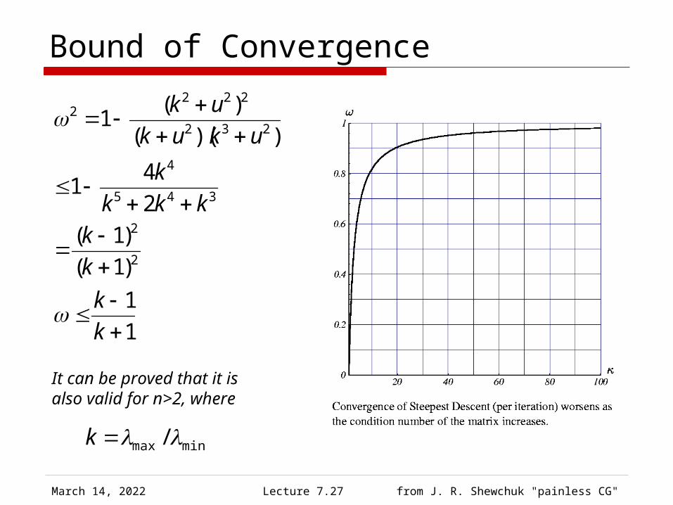
April 19, 2023 Lecture 7.27 from J. R. Shewchuk "painless CG"
Bound of Convergence
1
1
)1(
)1(
2
41
))((
)(1
2
2
345
4
232
2222
k
k
k
k
kkk
k
ukuk
uk
It can be proved that it is also valid for n>2, where
minmax /k
April 19, 2023 Lecture 7.28 figure from J. R. Shewchuk "painless CG"
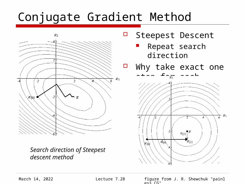
Conjugate Gradient Method Steepest Descent
Repeat search direction Why take exact one step
for each direction?
Search direction of Steepestdescent method
April 19, 2023 Lecture 7.29 Zhengyong (Simon) Zhu, UCSD
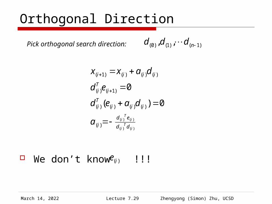
Orthogonal Direction
)()(
)()(
)(
)()()()(
)1()(
)()()()1(
0)(
0
iT
i
iT
i
dd
ed
i
iiiTi
iTi
iiii
a
daed
ed
daxx
We don’t know !!!
)1()1()0( ,, nddd Pick orthogonal search direction:
)(ie

April 19, 2023 Lecture 7.30 from J. R. Shewchuk "painless CG"
Orthogonal A-orthogonal Instead of orthogonal search direction, we make search
direction A –orthogonal (conjugate)
0)()( iTi Add

April 19, 2023 Lecture 7.31 Zhengyong (Simon) Zhu, UCSD
Search Step Size
0)()()( )()1()1()1()1( iT
iidadT
iidad dxfxxfxf
)()(
)()(
)(
)()()()()(
)()()()(
)()1(
)()1(
)()(
0))((
0)(
0
iT
i
iT
i
Add
dr
i
iT
iiiT
i
iT
iii
iT
i
iT
i
a
dAdadAxb
ddaxAb
dAxb
dr

April 19, 2023 Lecture 7.32 Zhengyong (Simon) Zhu, UCSD
Iteration finish in n steps
1
0)()0(
n
jjjde Initial error:
)(
)(
)(
)()()()()0()(
)()(
)()(
)()(
1
0)()()0()(
)()(
)0()(
kAdd
Aed
Add
daeAd
Add
Aed
k
kTkkj
Tk
jj
Tk
a
AddAddeAd
kT
k
kT
k
kT
k
k
iii
Tk
kT
k
Tk
1
)()(
1
0)()(
1
0)()(
1
0)()()0()(
n
ijjj
i
jjj
n
jjj
i
jjji
da
dada
daee
A-orthogonal
The error component at direction djis eliminated at step j. After n steps,all errors are eliminated.

April 19, 2023 Lecture 7.33 Zhengyong (Simon) Zhu, UCSD
Conjugate Search Direction How to construct A-orthogonal search
directions, given a set of n linear independent vectors.
Since the residue vector in steepest descent method is orthogonal, a good candidate to start with
110 ,,, nrrr

April 19, 2023 Lecture 7.34 Zhengyong (Simon) Zhu, UCSD
Construct Search Direction -1 In Steepest Descent Method
New residue is just a linear combination of previous residue and
Let
)()()()()()()1()1( )( iiiiiiii AdardaeAAer
)(,0)()( jirr jTi
)(ir
)1( iAd
},,,{ 110 ii rrrspanD
ii Dd )1(We have
},,,,{
},,,,{
)0(1
)0(2
)0()0(
)0(1
)0(2
)0()0(
rArAArrspan
dAdAAddspanDi
ii
Krylov SubSpace: repeatedly applying a matrix to a vector

April 19, 2023 Lecture 7.35 Zhengyong (Simon) Zhu, UCSD
Construct Search Direction -2
)0()0( rd let
1
0)()()(
i
kkikii drd For i > 0
10
1
0
1
)1()1(
)()(
)1(
)1(
)(
1
)()(1
)()(1
)()(
)1()()()()()()(
)()()()()()1()(
ji
ji
otherwise
jirr
jirr
Adr
rrrrAdra
Adrarrrr
iTi
iTi
i
i
i
Add
rr
aij
iTia
iTia
jTi
jTij
Tij
Tij
jTijj
Tij
Ti

April 19, 2023 Lecture 7.36 Zhengyong (Simon) Zhu, UCSD
Construct Search Direction -3
)1()()()( iiii drd
)1,()( iii let
then
)1()1(
)()(
)1()2()1()1()1(
)()(
)1()1(
)()(
)1()1(
)()(
)1(
1
iTi
iTi
iTiii
Ti
iTi
iTi
iTi
iTi
iTi
ii
rr
rr
rdrr
rr
rd
rr
Add
rra
can get next direction from the previous one, without saving them all.

April 19, 2023 Lecture 7.37 Zhengyong (Simon) Zhu, UCSD
Conjugate Gradient Algorithm
)()1()1()1(
)1(
)()()1()1(
)()()()1(
)(
)0()0()0(
)()(
)1()1(
)()(
)()(
iiii
rr
rr
i
iiii
iiii
Add
rr
i
drd
Adarr
daxx
a
Axbrd
iT
i
iT
i
iT
i
iT
i
Given x0, iterate until residue is smaller than error tolerance

April 19, 2023 Lecture 7.38 courtesy J.R.Gilbert, UCSB
Conjugate gradient: Convergence
In exact arithmetic, CG converges in n steps (completely unrealistic!!)
Accuracy after k steps of CG is related to: consider polynomials of degree k that are equal
to 1 at 0. how small can such a polynomial be at all the
eigenvalues of A? Thus, eigenvalues close together are good. Condition number: κ(A) = ||A||2 ||A-1||2 = λmax(A) /
λmin(A) Residual is reduced by a constant factor by
O(κ1/2(A)) iterations of CG.

April 19, 2023 Lecture 7.39 courtesy J.R.Gilbert, UCSB
Other Krylov subspace methods
Nonsymmetric linear systems: GMRES:
for i = 1, 2, 3, . . . find xi Ki (A, b) such that ri = (Axi – b) Ki (A, b)
But, no short recurrence => save old vectors => lots more space (Usually “restarted” every k iterations to use less space.)
BiCGStab, QMR, etc.:Two spaces Ki (A, b) and Ki (AT, b) w/ mutually orthogonal
bases Short recurrences => O(n) space, but less robust Convergence and preconditioning more delicate than CG Active area of current research
Eigenvalues: Lanczos (symmetric), Arnoldi (nonsymmetric)

April 19, 2023 Lecture 7.40 courtesy J.R.Gilbert, UCSB
Preconditioners Suppose you had a matrix B such that:
1. condition number κ(B-1A) is small2. By = z is easy to solve
Then you could solve (B-1A)x = B-1b instead of Ax = b
B = A is great for (1), not for (2) B = I is great for (2), not for (1) Domain-specific approximations sometimes work B = diagonal of A sometimes works
Better: blend in some direct-methods ideas. . .

April 19, 2023 Lecture 7.41 courtesy J.R.Gilbert, UCSB
Preconditioned conjugate gradient iteration
x0 = 0, r0 = b, d0 = B-1 r0, y0 = B-1 r0
for k = 1, 2, 3, . . .
αk = (yTk-1rk-1) / (dT
k-1Adk-1) step length
xk = xk-1 + αk dk-1 approx solution
rk = rk-1 – αk Adk-1 residual
yk = B-1 rk preconditioning solve
βk = (yTk rk) / (yT
k-1rk-1) improvement
dk = yk + βk dk-1 search direction One matrix-vector multiplication per iteration One solve with preconditioner per iteration

April 19, 2023 Lecture 7.42 Zhengyong (Simon) Zhu, UCSD
Outline Iterative Method
Stationary Iterative Method (SOR, GS,Jacob) Krylov Method (CG, GMRES) Multigrid Method

April 19, 2023 Lecture 7.43 Zhengyong (Simon) Zhu, UCSD
What is the multigrid A multilevel iterative method to solve
Ax=b Originated in PDEs on geometric grids Expend the multigrid idea to unstructure
d problem – Algebraic MG Geometric multigrid for presenting the b
asic ideas of the multigrid method.
April 19, 2023 Lecture 7.44 Zhengyong (Simon) Zhu, UCSD
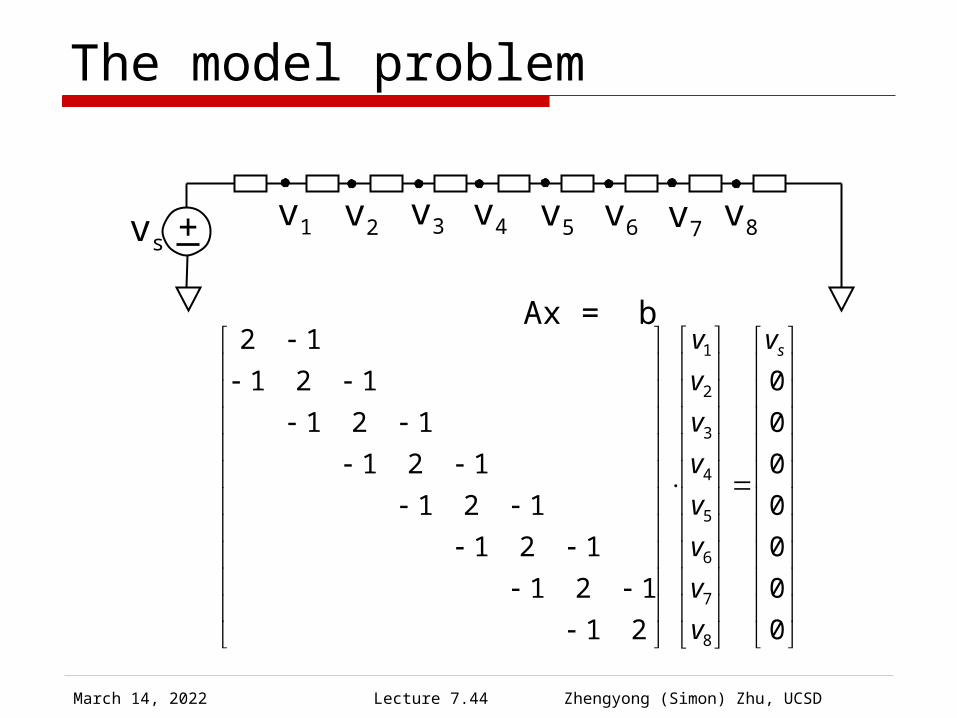
The model problem
+ v1 v2 v3 v4 v5 v6 v7 v8vs
0
0
0
0
0
0
0
21
121
121
121
121
121
121
12
8
7
6
5
4
3
2
1 sv
v
v
v
v
v
v
v
v Ax = b

April 19, 2023 Lecture 7.45 Zhengyong (Simon) Zhu, UCSD
Simple iterative method x(0) -> x(1) -> … -> x(k) Jacobi iteration
Matrix form : x(k) = Rjx(k-1) + Cj
General form: x(k) = Rx(k-1) + C (1) Stationary: x* = Rx* + C (2)
))(/1(1
)(1
1
)()1(
n
ij
kjik
i
j
kjikiii
ki xaxabax

April 19, 2023 Lecture 7.46 Zhengyong (Simon) Zhu, UCSD
Error and Convergence
Definition: error e = x* - x (3) residual r = b – Ax (4)
e, r relation: Ae = r (5) ((3)+(4))
e(1) = x*-x(1) = Rx* + C – Rx(0) – C =Re(0) Error equation e(k) = Rke(0) (6) ((1)+(2)+(3))
Convergence:0lim )(
k
ke

April 19, 2023 Lecture 7.47 Zhengyong (Simon) Zhu, UCSD
Error of diffenent frequency Wavenumber k and frequency
= k/n
• High frequency error is more oscillatory between points
k= 1
k= 4 k= 2

April 19, 2023 Lecture 7.48 Zhengyong (Simon) Zhu, UCSD
Iteration reduce low frequency error efficiently
Smoothing iteration reduce high frequency error efficiently, but not low frequency error
Error
Iterations
k = 1
k = 2
k = 4

April 19, 2023 Lecture 7.49 Zhengyong (Simon) Zhu, UCSD
Multigrid – a first glance Two levels : coarse and fine grid
1 2 3 4 5 6 7 8
1 2 3 4 A2hx2h=b2h
Ahxh=bhh
Ax=b
2h

April 19, 2023 Lecture 7.50 Zhengyong (Simon) Zhu, UCSD
Idea 1: the V-cycle iteration
Also called the nested iteration
A2hx2h = b2h A2hx2h = b2h
h
2h
Ahxh = bh
Iterate =>
)0(2holdx
)0(2hnewx
Start with
Prolongation: )0(2hnewx )0(h
oldx Restriction: )0(hnewx )1(2h
oldx
Iterate to get )0(hnewx
Question 1: Why we need the coarse grid ?
April 19, 2023 Lecture 7.51 Zhengyong (Simon) Zhu, UCSD
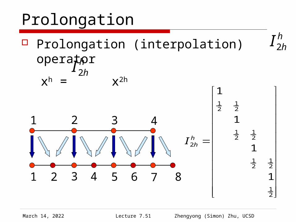
Prolongation Prolongation (interpolation) operator
xh = x2h
1 2 3 4 5 6 7 8
1 2 3 4
hhI2
hhI2
21
21
21
21
21
21
21
2
1
1
1
1
hhI

April 19, 2023 Lecture 7.52 Zhengyong (Simon) Zhu, UCSD
Restriction Restriction operator
xh = x2h
hhI2
hhI2
12
1 12 22
1 12 2
1 12 2
1
1
1
1
hhI
1 2 3 4 5 6 7 8
1 2 3 4

April 19, 2023 Lecture 7.53 Zhengyong (Simon) Zhu, UCSD
Smoothing The basic iterations in each level
In ph: xphold xph
new
Iteration reduces the error, makes the error smooth geometrically.So the iteration is called smoothing.
April 19, 2023 Lecture 7.54 Zhengyong (Simon) Zhu, UCSD
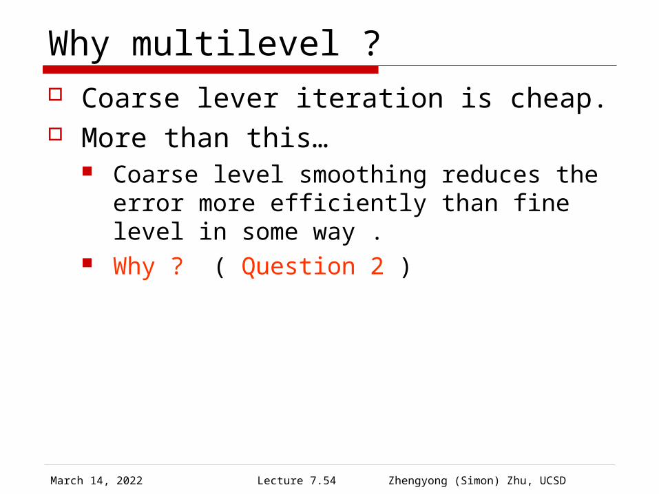
Why multilevel ? Coarse lever iteration is cheap. More than this…
Coarse level smoothing reduces the error more efficiently than fine level in some way .
Why ? ( Question 2 )
April 19, 2023 Lecture 7.55 Zhengyong (Simon) Zhu, UCSD
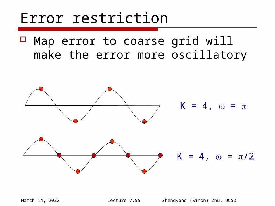
Error restriction Map error to coarse grid will make the
error more oscillatory
K = 4, = /2
K = 4, =

April 19, 2023 Lecture 7.56 Zhengyong (Simon) Zhu, UCSD
Idea 2: Residual correction
Known current solution x
Solve Ax=b eq. to
MG do NOT map x directly between levels
Map residual equation to coarse level1. Calculate rh
2. b2h= Ih2h rh ( Restriction )
3. eh = Ih2h
x2h ( Prolongation )4. xh = xh + eh
**
*
exx
rAeSolve

April 19, 2023 Lecture 7.57 Zhengyong (Simon) Zhu, UCSD
Why residual correction ? Error is smooth at fine level, but the
actual solution may not be. Prolongation results in a smooth error
in fine level, which is suppose to be a good evaluation of the fine level error.
If the solution is not smooth in fine level, prolongation will introduce more high frequency error.

April 19, 2023 Lecture 7.58 Zhengyong (Simon) Zhu, UCSD
`
Revised V-cycle with idea 2
Smoothing on xh
Calculate rh
b2h= Ih2h rh
Smoothing on x2h
eh = Ih2h
x2h
Correct: xh = xh + eh
Restriction
Prolongation
2h h

April 19, 2023 Lecture 7.59 Zhengyong (Simon) Zhu, UCSD
What is A2h
Galerkin condition
hh
hhh
h IAIA 222
hhhhhh
hhh
hhh
hhhh
hhhhhh
h
bxArIxIAI
rxIAeAxIe22222
22
22
22

April 19, 2023 Lecture 7.60 Zhengyong (Simon) Zhu, UCSD
Going to multilevels
V-cycle and W-cycle
Full Multigrid V-cycle
h
2h
4h
h
2h
4h
8h

April 19, 2023 Lecture 7.61 Zhengyong (Simon) Zhu, UCSD
Performance of Multigrid Complexity comparison
Gaussian elimination O(N2)
Jacobi iteration O(N2log)
Gauss-Seidel O(N2log)
SOR O(N3/2log)
Conjugate gradient O(N3/2log)
Multigrid ( iterative ) O(Nlog)Multigrid ( FMG ) O(N)

April 19, 2023 Lecture 7.62 Zhengyong (Simon) Zhu, UCSD
Summary of MG ideas
Three important ideas of MG1. Nested iteration2. Residual correction3. Elimination of error:
high frequency : fine grid low frequency : coarse grid

April 19, 2023 Lecture 7.63 Zhengyong (Simon) Zhu, UCSD
AMG :for unstructured grids Ax=b, no regular grid structure Fine grid defined from A
1
2
3 4
5 6
311000
130010
102001
000411
010131
001113
A

April 19, 2023 Lecture 7.64 Zhengyong (Simon) Zhu, UCSD
Three questions for AMG How to choose coarse grid
How to define the smoothness of errors
How are interpolation and prolongation done

April 19, 2023 Lecture 7.65 Zhengyong (Simon) Zhu, UCSD
How to choose coarse grid Idea:
C/F splitting As few coarse grid
point as possible For each F-node, at
least one of its neighbor is a C-node
Choose node with strong coupling to other nodes as C-node
1
2
3 4
5 6

April 19, 2023 Lecture 7.66 Zhengyong (Simon) Zhu, UCSD
How to define the smoothness of error
AMG fundamental concept: Smooth error = small residuals ||r|| << ||e||

April 19, 2023 Lecture 7.67 Zhengyong (Simon) Zhu, UCSD
How are Prolongation and Restriction done
Prolongation is based on smooth error and strong connections
Common practice: I

April 19, 2023 Lecture 7.68 Zhengyong (Simon) Zhu, UCSD
AMG Prolongation (2)

April 19, 2023 Lecture 7.69 Zhengyong (Simon) Zhu, UCSD
AMG Prolongation (3)
Thh
hh ICI )( 22
Restriction :

April 19, 2023 Lecture 7.70 Zhengyong (Simon) Zhu, UCSD
Summary Multigrid is a multilevel iterative
method. Advantage: scalable If no geometrical grid is available, try
Algebraic multigrid method

April 19, 2023 Lecture 7.71 courtesy J.R.Gilbert, UCSB
Pivoting
LU
GMRES,
BiCGSTAB, …
Cholesky
Conjugate gradient
MultiGrid
DirectA = LU
Iterativey’ = Ay
Non-symmetric
Symmetricpositivedefinite
More Robust Less Storage (if sparse)
More Robust
More General
The landscape of Solvers


