CSE 520 Computer Architecture Lec 4 – Quantifying Cost, Energy-Consumption, Performance, and Dependability (Chapter 1) Sandeep K. S. Gupta School of Computing and Informatics Arizona State University Based on Slides by David Patterson and M. Younis
Transcript
CSE 520 Computer Architecture
Lec 4 – Quantifying Cost, Energy-
Consumption, Performance, and
Dependability (Chapter 1)
Sandeep K. S. GuptaSchool of Computing and Informatics
Arizona State University
Based on Slides by David Patterson and M. Younis
CSE 520 Fall 2007 2
Moore’s Law gets life-term extension
• “Intel, IBM unveil new chip technology - Breakthrough, using new material, will allow processors to become smaller and more powerful” – CNN Money http://money.cnn.com/2007/01/27/technology/bc.microchips.reut/index.htm?cnn=yes
– “Intel Corp. and IBM have announced one of the biggest advances in transistors in four decades, overcoming a frustrating obstacle by ensuring microchips can get even smaller and more powerful.”
– “The latest breakthrough means Intel, IBM and others can proceed with technology roadmaps that call for the next generation of chips to be made with circuitry as small as 45 nanometers, about 1/2000th the width of a human hair.”
– “Researchers are optimistic the new technology can be used at least through two more technology generations out, when circuitry will be just 22 nanometers. “
• “This gives the entire chip industry a new life in terms of Moore’s Law, in all three of the big metrics – performance, power consumption, and transistor density,” – David Lammers, director, WeSRCH.com – social networking site for semiconductor enthusiasts (part of VLSI Research Inc.)
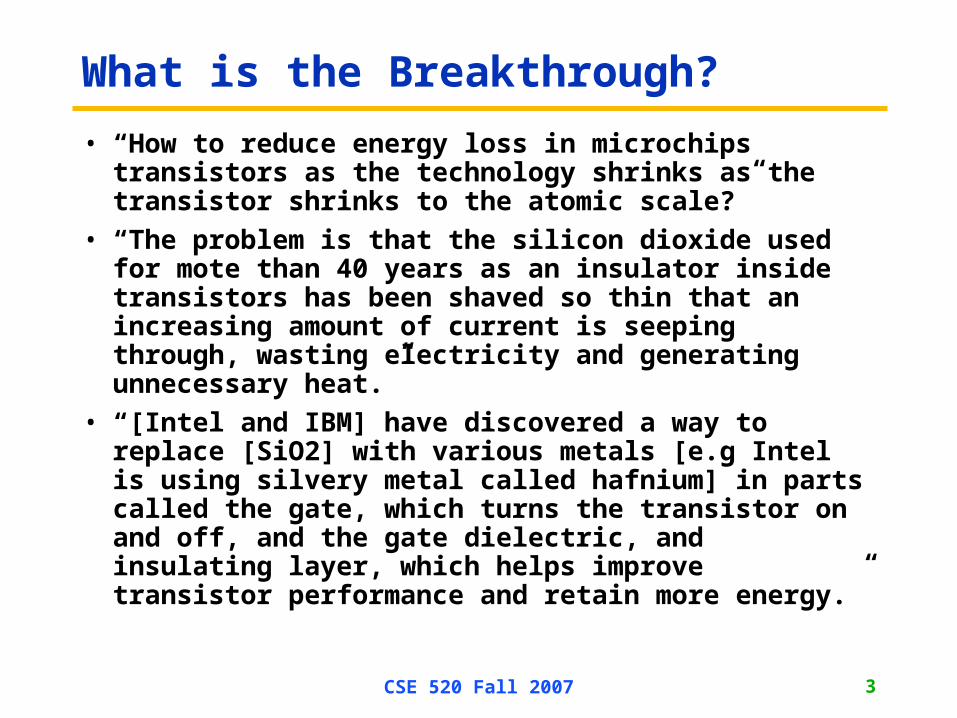
• “How to reduce energy loss in microchips transistors as the technology shrinks as the transistor shrinks to the atomic scale?”
• “The problem is that the silicon dioxide used for mote than 40 years as an insulator inside transistors has been shaved so thin that an increasing amount of current is seeping through, wasting electricity and generating unnecessary heat.”
• “[Intel and IBM] have discovered a way to replace [SiO2] with various metals [e.g Intel is using silvery metal called hafnium] in parts called the gate, which turns the transistor on and off, and the gate dielectric, and insulating layer, which helps improve transistor performance and retain more energy.”
CSE 520 Fall 2007 4
What does it mean for Intel and Arizona?
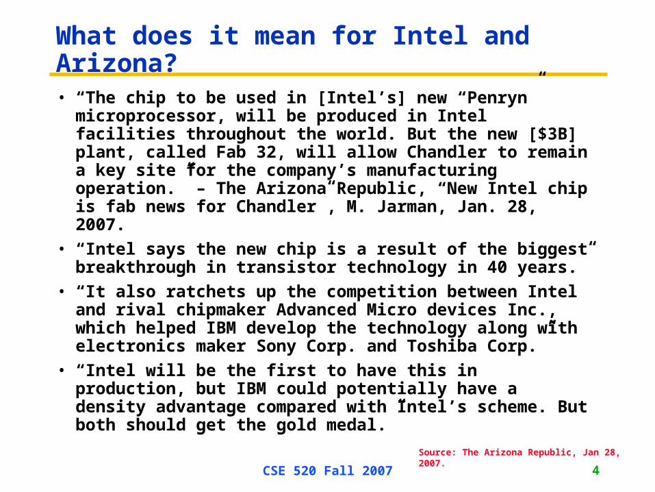
• “The chip to be used in [Intel’s] new “Penryn” microprocessor, will be produced in Intel facilities throughout the world. But the new [$3B] plant, called Fab 32, will allow Chandler to remain a key site for the company’s manufacturing operation.” – The Arizona Republic, “New Intel chip is fab news for Chandler”, M. Jarman, Jan. 28, 2007.
• “Intel says the new chip is a result of the biggest breakthrough in transistor technology in 40 years.”
• “It also ratchets up the competition between Intel and rival chipmaker Advanced Micro devices Inc., which helped IBM develop the technology along with electronics maker Sony Corp. and Toshiba Corp.”
• “Intel will be the first to have this in production, but IBM could potentially have a density advantage compared with Intel’s scheme. But both should get the gold medal.”
Source: The Arizona Republic, Jan 28, 2007.
CSE 520 Fall 2007 5
Recap
• Execution (CPU) time is the only true measure of performance.
• One must be careful when using other measures such as MIPS.
• Computer architects (Industry) need to be aware of Technology trends to design computer architectures which address the various “walls”.
• Increasing proportion of Static (or leakage) current (in comparison to Dynamic current) is a cause of concern
• One of the motivation for multicore design is to reduce Thermal dissipation
CSE 520 Fall 2007 6
A common theme in Hardware design is to make the common case fast
Increasing the clock rate would not affect memory access time
Using a floating point processing unit does not speed integer ALU operations
Example: Floating point instructions improved to run 2 times faster; but only 10% of the actual instructions are floating point
Exec-Timenew = Exec-Timeold x (0.9 + .1/2) = 0.95 x Exec-Timeold
The performance enhancement possible with a given improvement is limited by the amount that the improved feature is used
unaffected timeExecution
timprovemen ofAmount
timprovemen by the affected timeExecution
t improvemenafter timeExecution
unaffected timeExecution
timprovemen ofAmount
timprovemen by the affected timeExecution
t improvemenafter timeExecution
Amdahl’s Law
Slide by M. Younis
CSE 520 Fall 2007 7
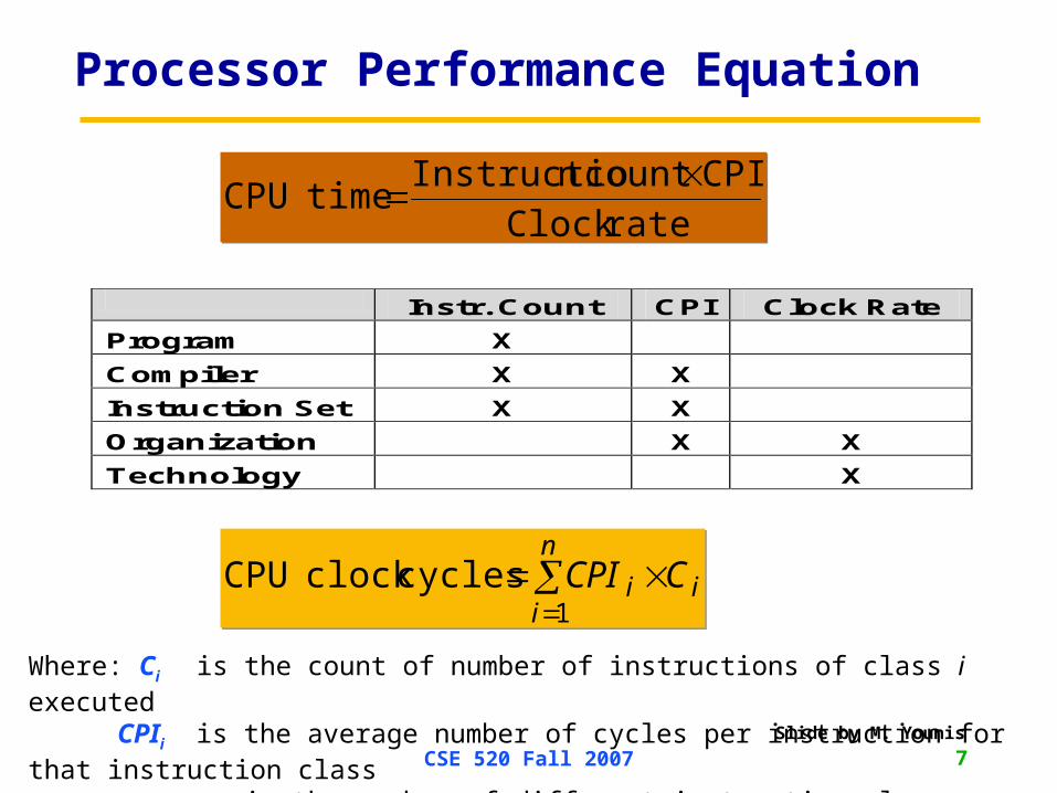
Processor Performance Equation
rate Clock
CPIcount nInstructiotime CPU
rate Clock
CPIcount nInstructiotime CPU
Instr. Count CPI Clock Rate
Program X
Compiler X X
Instruction Set X X
Organization X X
Technology X
i
n
ii CCPI
1cycles clock CPU i
n
ii CCPI
1cycles clock CPU
Where: Ci is the count of number of instructions of class i executed CPIi is the average number of cycles per instruction for that instruction class n is the number of different instruction classes Slide by M. Younis
CSE 520 Fall 2007 8
Performance Metrics - Summary
Maximizing performance means
minimizing response (execution) time timeExecution
1ePerformanc
timeExecution
1ePerformanc
Compiler
Programming Language
Application
Datapath
Control
Transistors Wires Pins
ISA
Function Units
(millions) of Instructions per second: MIPS(millions) of (FP) operations per second: MFLOP/s
Cycles per second (clock rate)
Megabytes per second
Operations per second
Designer
User
* Figure is courtesy of Dave Patterson
CSE 520 Fall 2007 9
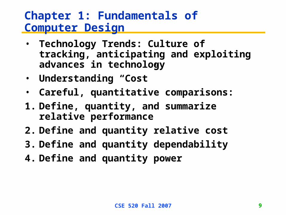
Chapter 1: Fundamentals of Computer Design• Technology Trends: Culture of tracking,
anticipating and exploiting advances in technology
• Understanding “Cost”
• Careful, quantitative comparisons:
1. Define, quantity, and summarize relative performance
2. Define and quantity relative cost
3. Define and quantity dependability
4. Define and quantity power
CSE 520 Fall 2007 10
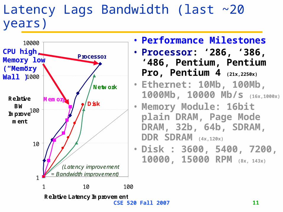
Moore’s Law: 2X transistors / “year”
• “Cramming More Components onto Integrated Circuits”– Gordon Moore, Electronics, 1965
• # on transistors / cost-effective integrated circuit double every N months (12 ≤ N ≤ 24)
• In the time that bandwidth doubles, latency improves by no more than a factor of 1.2 to 1.4
(and capacity improves faster than bandwidth)
• Stated alternatively: Bandwidth improves by more than the square of the improvement in Latency
CSE 520 Fall 2007 13
6 Reasons Latency Lags Bandwidth
1. Moore’s Law helps BW more than latency
2. Distance limits latency
3. Bandwidth easier to sell (“bigger=better”)
4. Latency helps BW, but not vice versa
5. Bandwidth hurts latency
6. Operating System overhead hurts Latency more than Bandwidth
CSE 520 Fall 2007 14
Summary of Technology Trends
• For disk, LAN, memory, and microprocessor, bandwidth improves by square of latency improvement
– In the time that bandwidth doubles, latency improves by no more than 1.2X to 1.4X
• Lag probably even larger in real systems, as bandwidth gains multiplied by replicated components
– Multiple processors in a cluster or even in a chip
– Multiple disks in a disk array
– Multiple memory modules in a large memory
– Simultaneous communication in switched LAN
• HW and SW developers should innovate assuming Latency Lags Bandwidth
– If everything improves at the same rate, then nothing really changes
– When rates vary, require real innovation
CSE 520 Fall 2007 15
Chapter 1: Fundamentals of Computer Design• Technology Trends: Culture of tracking,
anticipating and exploiting advances in technology
• Understanding “Cost”
• Careful, quantitative comparisons:
1. Define, quantity, and summarize relative performance
2. Define and quantity relative cost
3. Define and quantity dependability
4. Define and quantity power
CSE 520 Fall 2007 16
Trends in Cost
• Textbooks usually ignore cost half of cost-performance because costs change.
• Yet understanding cost and its factors is essential for designer’s to make intelligent decisions about what features to include in designs when costs is an issue
• Agenda: Study impact of time, volume and commodification
• Underlying principle: learning curve – manufacturing costs decrease over time
– Measured by change in yield – the percentage of manufactured devices that survives the testing procedure
CSE 520 Fall 2007 17
Integrated Circuits: Fueling Innovation
Year Technology used in computers Relative performance/unit cost1951 Vacuum tube 11965 Transistor 351975 Integrated circuits 9001995 Very large-scale integrated circuit 2,400,000
• Chip manufacturing begins with silicon, a substance found in sand
• Silicon does not conduct electricity well and thus called semiconductor
• A special chemical process can transform tiny areas of silicon to either:1. Excellent conductors of electricity (like copper)2. Excellent insulator from electricity (like glass)3. Areas that can conduct or insulate under a special condition (a switch)
• A transistor is simply an on/off switch controlled by electricity
• Integrated circuits combines dozens of hundreds of transistors in a chip
Advances of the IC technology affect H/W and S/W design philosophyAdvances of the IC technology affect H/W and S/W design philosophy
CSE 520 Fall 2007 18
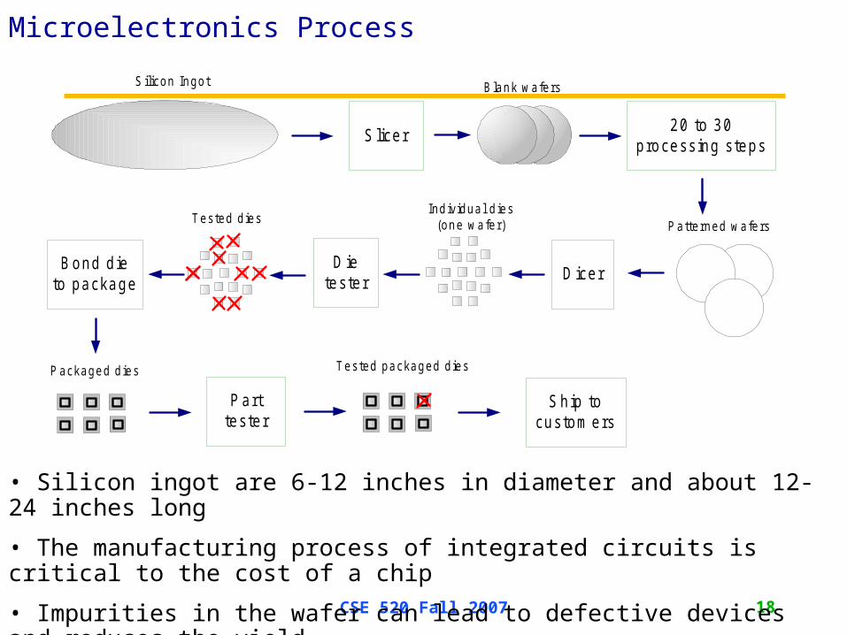
Slicer20 to 30
processing steps
D icerD ie
testerBond die
to package
Parttester
Ship tocustom ers
Packaged dies Tested packaged dies
Patterned wafersIndividual d ies
(one wafer)Tested d ies
S ilicon Ingot B lank wafers
Microelectronics Process
• Silicon ingot are 6-12 inches in diameter and about 12-24 inches long
• The manufacturing process of integrated circuits is critical to the cost of a chip
• Impurities in the wafer can lead to defective devices and reduces the yield
CSE 520 Fall 2007 19
Integrated Circuits Costs
Area Die2
diameter- Wafer
Area Die
)diameter/2-(Wafer per Wafer Dies
2
Die_Area*a r_unit_areDefects_pe
1 dWafer yiel YieldDie-
Die cost roughly goes with die area4
Die cost roughly goes with die area4
Test Yield Final
Cost PackingCost TestingCost DieCost IC
Yield DieWafer per Dies
CostWafer Cost Die
* Slide is courtesy of Dave Patterson
CSE 520 Fall 2007 20
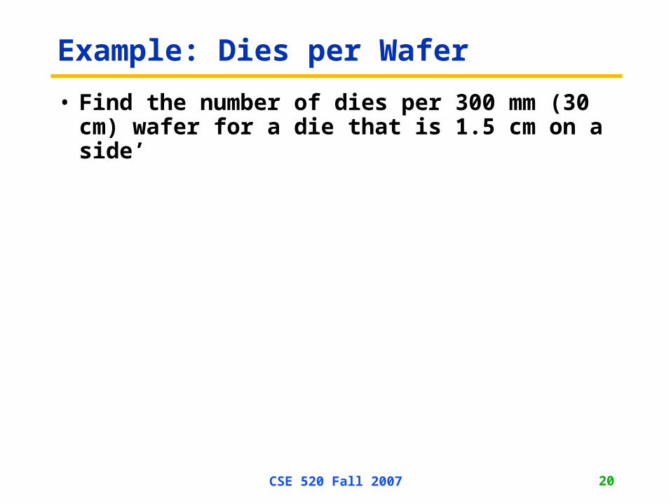
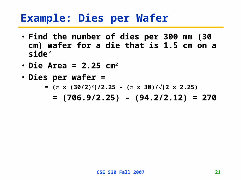
Example: Dies per Wafer
• Find the number of dies per 300 mm (30 cm) wafer for a die that is 1.5 cm on a side’
CSE 520 Fall 2007 21
Example: Dies per Wafer
• Find the number of dies per 300 mm (30 cm) wafer for a die that is 1.5 cm on a side’
• Die Area = 2.25 cm2
• Dies per wafer = = ( x (30/2)2)/2.25 – ( x 30)/(2 x 2.25)
= (706.9/2.25) – (94.2/2.12) = 270
CSE 520 Fall 2007 22
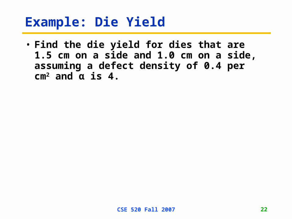
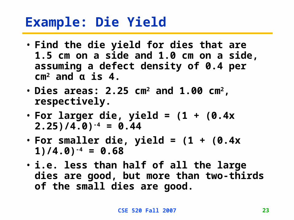
Example: Die Yield
• Find the die yield for dies that are 1.5 cm on a side and 1.0 cm on a side, assuming a defect density of 0.4 per cm2 and α is 4.
CSE 520 Fall 2007 23
Example: Die Yield
• Find the die yield for dies that are 1.5 cm on a side and 1.0 cm on a side, assuming a defect density of 0.4 per cm2 and α is 4.
• Dies areas: 2.25 cm2 and 1.00 cm2, respectively.
• i.e. less than half of all the large dies are good, but more than two-thirds of the small dies are good.
CSE 520 Fall 2007 24
Real World Examples
From "Estimating IC Manufacturing Costs,” by Linley Gwennap, Microprocessor Report, August 2, 1993, p. 15
Chip Layers Wafer cost Defect/cm2 Area (mm2) Dies/Wafer Yield Die Cost
386DX 2 $900 1.0 43 360 71% $4
486DX2 3 $1200 1.0 81 181 54% $12
PowerPC 601 4 $1700 1.3 121 115 28% $53
HP PA 7100 3 $1300 1.0 196 66 27% $73
DEC Alpha 3 $1500 1.2 234 53 19% $149
SuperSPARC 3 $1700 1.6 256 48 13% $272
Pentium 3 $1500 1.5 296 40 9% $417
* Slide is courtesy of Dave Patterson
CSE 520 Fall 2007 25
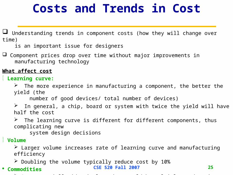
Costs and Trends in Cost
Understanding trends in component costs (how they will change over time) is an important issue for designers
Component prices drop over time without major improvements in manufacturing technology
What affect cost Learning curve:
The more experience in manufacturing a component, the better the yield (the number of good devices/ total number of devices) In general, a chip, board or system with twice the yield will have half the cost The learning curve is different for different components, thus complicating new system design decisions
Volume Larger volume increases rate of learning curve and manufacturing efficiency Doubling the volume typically reduce cost by 10%
Commodities Are essentially identical products sold by multiple vendors in large volumes Aid the competition and drive the efficiency higher and thus the cost down
CSE 520 Fall 2007 26
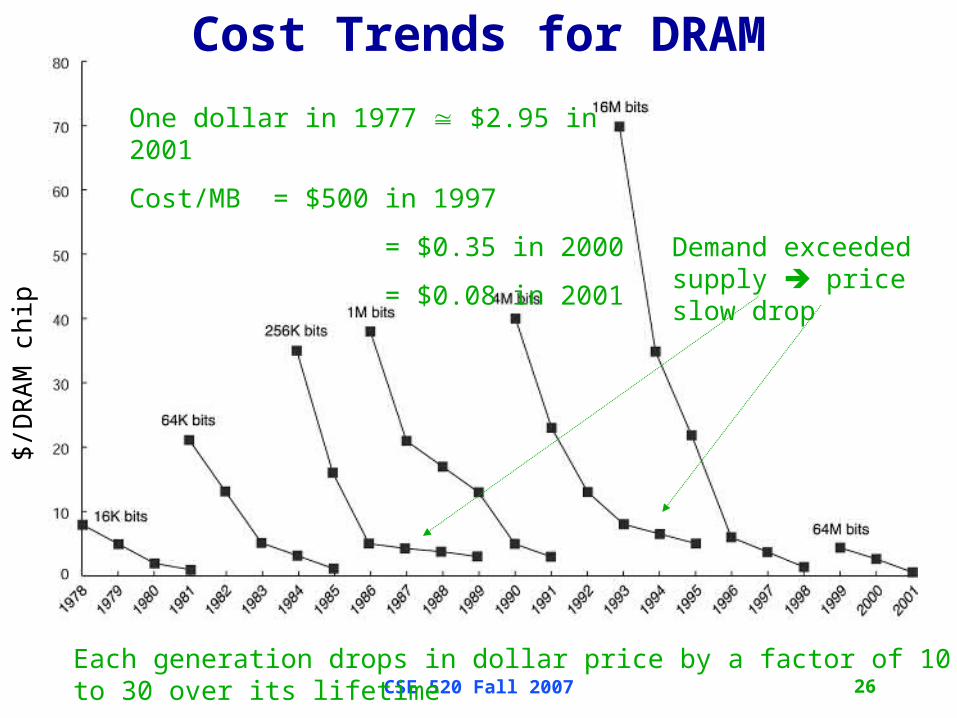
$/D
RA
M c
hip
Cost Trends for DRAM
One dollar in 1977 $2.95 in 2001
Cost/MB = $500 in 1997
= $0.35 in 2000
= $0.08 in 2001Demand exceeded supply price slow drop
Each generation drops in dollar price by a factor of 10 to 30 over its lifetime
CSE 520 Fall 2007 27
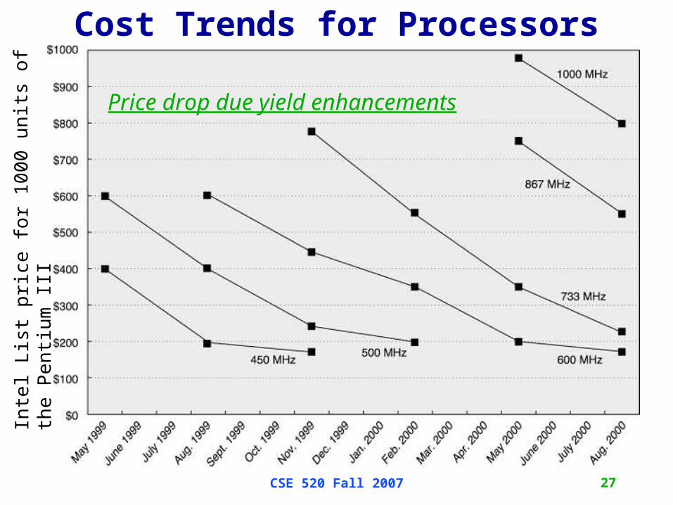
Cost Trends for ProcessorsIn
tel L
ist p
rice
for
10
00 u
nits
of t
he
Pe
ntiu
m II
I
Price drop due yield enhancements
CSE 520 Fall 2007 28
Cost vs. Price
Component Costs: raw material cost for the system’s building blocks
Direct Costs (add 25% to 40%) recurring costs: labor, purchasing, scrap, warranty
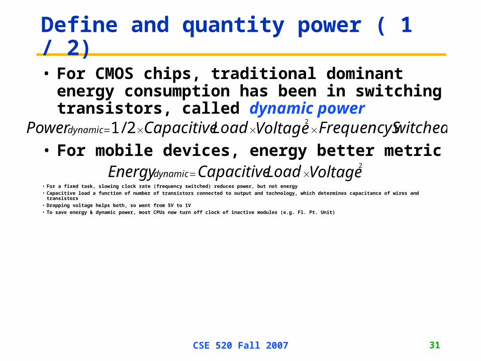
• For mobile devices, energy better metricVoltageLoadCapacitiveEnergydynamic
2
• For a fixed task, slowing clock rate (frequency switched) reduces power, but not energy
• Capacitive load a function of number of transistors connected to output and technology, which determines capacitance of wires and transistors
• Dropping voltage helps both, so went from 5V to 1V
• To save energy & dynamic power, most CPUs now turn off clock of inactive modules (e.g. Fl. Pt. Unit)
CSE 520 Fall 2007 32
Example of quantifying power
• Suppose 15% reduction in voltage results in a 15% reduction in frequency. What is impact on dynamic power?
dynamic
dynamic
dynamic
OldPower
OldPower
witchedFrequencySVoltageLoadCapacitive
witchedFrequencySVoltageLoadCapacitivePower
6.0
)85(.
)85(.85.2/1
2/1
3
2
2
CSE 520 Fall 2007 33
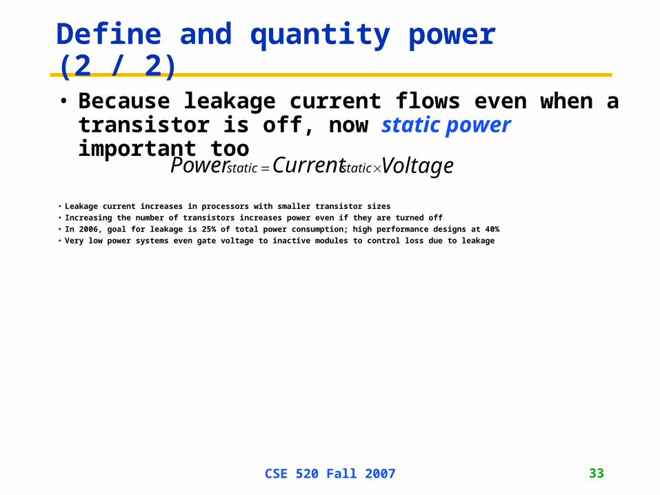
Define and quantity power (2 / 2)
• Because leakage current flows even when a transistor is off, now static power important too
• Leakage current increases in processors with smaller transistor sizes
• Increasing the number of transistors increases power even if they are turned off
• In 2006, goal for leakage is 25% of total power consumption; high performance designs at 40%
• Very low power systems even gate voltage to inactive modules to control loss due to leakage
VoltageCurrentPower staticstatic
CSE 520 Fall 2007 34
Outline
• Review
• Technology Trends: Culture of tracking, anticipating and exploiting advances in technology
• Careful, quantitative comparisons:
1. Define and quantity power
2. Define and quantity dependability
3. Define, quantity, and summarize relative performance
4. Define and quantity relative cost
CSE 520 Fall 2007 35
Define and quantity dependability (1/3)
• How decide when a system is operating properly?
• Infrastructure providers now offer Service Level Agreements (SLA) to guarantee that their networking or power service would be dependable
• Systems alternate between 2 states of service with respect to an SLA:
1. Service accomplishment, where the service is delivered as specified in SLA
2. Service interruption, where the delivered service is different from the SLA
• Failure = transition from state 1 to state 2
• Restoration = transition from state 2 to state 1
CSE 520 Fall 2007 36
Define and quantity dependability (2/3)
• Module reliability = measure of continuous service accomplishment (or time to failure). 2 metrics
1. Mean Time To Failure (MTTF) measures Reliability
2. Failures In Time (FIT) = 1/MTTF, the rate of failures • Traditionally reported as failures per billion hours of operation
• Mean Time To Repair (MTTR) measures Service Interruption– Mean Time Between Failures (MTBF) = MTTF+MTTR
• Module availability measures service as alternate between the 2 states of accomplishment and interruption (number between 0 and 1, e.g. 0.9)
• Module availability = MTTF / ( MTTF + MTTR)
CSE 520 Fall 2007 37
Example calculating reliability
• If modules have exponentially distributed lifetimes (age of module does not affect probability of failure), overall failure rate is the sum of failure rates of the modules
• Calculate FIT and MTTF for 10 disks (1M hour MTTF per disk), 1 disk controller (0.5M hour MTTF), and 1 power supply (0.2M hour MTTF):
MTTF
eFailureRat
CSE 520 Fall 2007 39
Outline
• Review
• Technology Trends: Culture of tracking, anticipating and exploiting advances in technology
• Careful, quantitative comparisons:
1. Define and quantity power
2. Define and quantity dependability
3. Define, quantity, and summarize relative performance
4. Define and quantity relative cost
CSE 520 Fall 2007 40
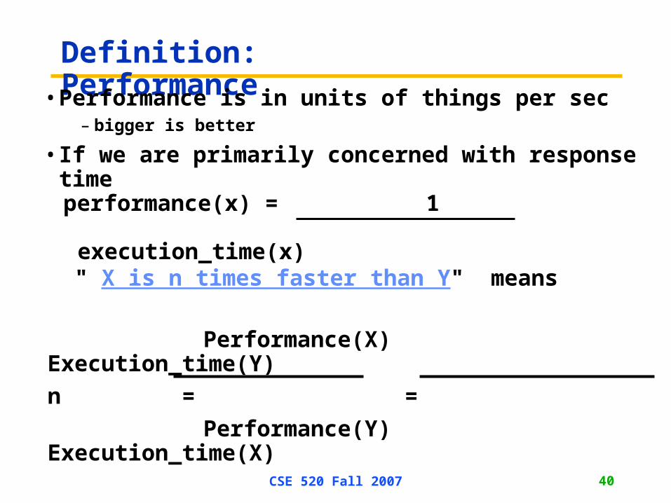
Performance(X) Execution_time(Y)
n = =
Performance(Y) Execution_time(X)
Definition: Performance• Performance is in units of things per sec
– bigger is better
• If we are primarily concerned with response time
performance(x) = 1 execution_time(x)
" X is n times faster than Y" means
CSE 520 Fall 2007 41
Performance: What to measure
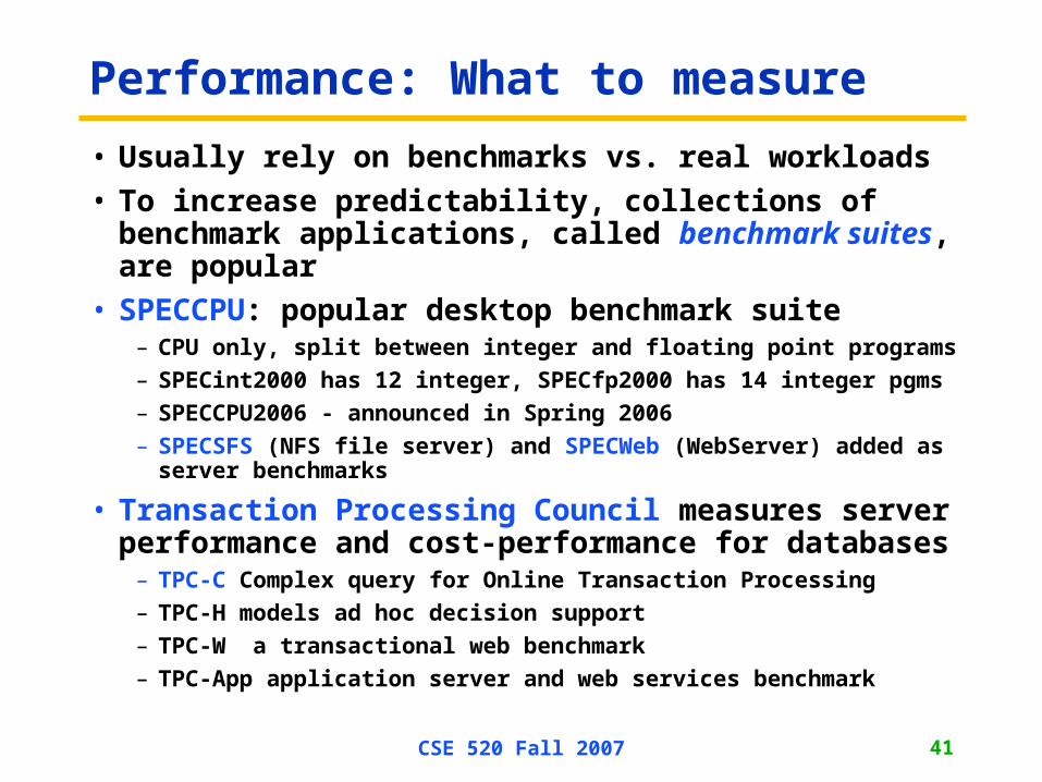
• Usually rely on benchmarks vs. real workloads
• To increase predictability, collections of benchmark applications, called benchmark suites, are popular
• SPECCPU: popular desktop benchmark suite– CPU only, split between integer and floating point programs
– SPECint2000 has 12 integer, SPECfp2000 has 14 integer pgms
– SPECCPU2006 - announced in Spring 2006
– SPECSFS (NFS file server) and SPECWeb (WebServer) added as server benchmarks
• Transaction Processing Council measures server performance and cost-performance for databases
– TPC-C Complex query for Online Transaction Processing
– TPC-H models ad hoc decision support
– TPC-W a transactional web benchmark
– TPC-App application server and web services benchmark
CSE 520 Fall 2007 42
Performance Tuning Cycle
Workload
Benchmarks
Independent Software Vendors
Evaluation:
Simulation/Silicon
Satisfactory?
OK
H/W or S/W changes
Product
No
Based on talk with Jim Abele, Intel Chandler (8/30/07)
CSE 520 Fall 2007 43
Some Comments
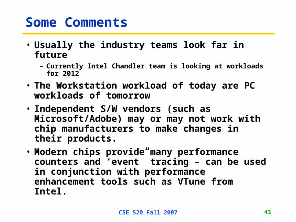
• Usually the industry teams look far in future– Currently Intel Chandler team is looking at workloads for 2012
• The Workstation workload of today are PC workloads of tomorrow
• Independent S/W vendors (such as Microsoft/Adobe) may or may not work with chip manufacturers to make changes in their products.
• Modern chips provide many performance counters and ‘event” tracing – can be used in conjunction with performance enhancement tools such as VTune from Intel.
CSE 520 Fall 2007 44
How Summarize Suite Performance (1/5)
• Arithmetic average of execution time of all pgms?– But they vary by 4X in speed, so some would be more important
than others in arithmetic average
• Could add a weights per program, but how pick weight?
– Different companies want different weights for their products
• SPECRatio: Normalize execution times to reference computer, yielding a ratio proportional to performance =
time on reference computer
time on computer being rated
CSE 520 Fall 2007 45
How Summarize Suite Performance (2/5)
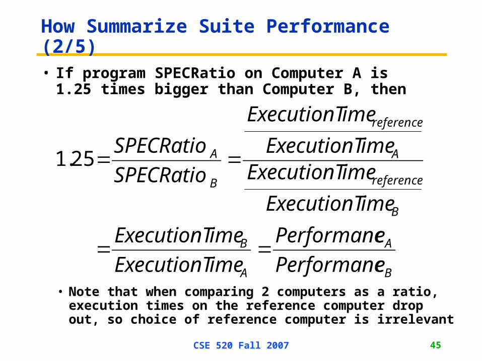
• If program SPECRatio on Computer A is 1.25 times bigger than Computer B, then
B
A
A
B
B
reference
A
reference
B
A
ePerformanc
ePerformanc
imeExecutionT
imeExecutionT
imeExecutionT
imeExecutionTimeExecutionT
imeExecutionT
SPECRatio
SPECRatio
25.1
• Note that when comparing 2 computers as a ratio, execution times on the reference computer drop out, so choice of reference computer is irrelevant
CSE 520 Fall 2007 46
How Summarize Suite Performance (3/5)
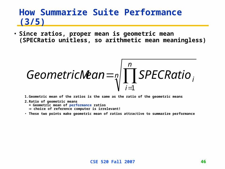
• Since ratios, proper mean is geometric mean (SPECRatio unitless, so arithmetic mean meaningless)
n
n
iiSPECRatioeanGeometricM
1
1. Geometric mean of the ratios is the same as the ratio of the geometric means
2. Ratio of geometric means = Geometric mean of performance ratios choice of reference computer is irrelevant!
• These two points make geometric mean of ratios attractive to summarize performance
CSE 520 Fall 2007 47
How Summarize Suite Performance (4/5)
• Does a single mean well summarize performance of programs in benchmark suite?
• Can decide if mean a good predictor by characterizing variability of distribution using standard deviation
• Like geometric mean, geometric standard deviation is multiplicative rather than arithmetic
• Can simply take the logarithm of SPECRatios, compute the standard mean and standard deviation, and then take the exponent to convert back:
i
n
i
i
SPECRatioStDevtDevGeometricS
SPECRation
eanGeometricM
lnexp
ln1
exp1
CSE 520 Fall 2007 48
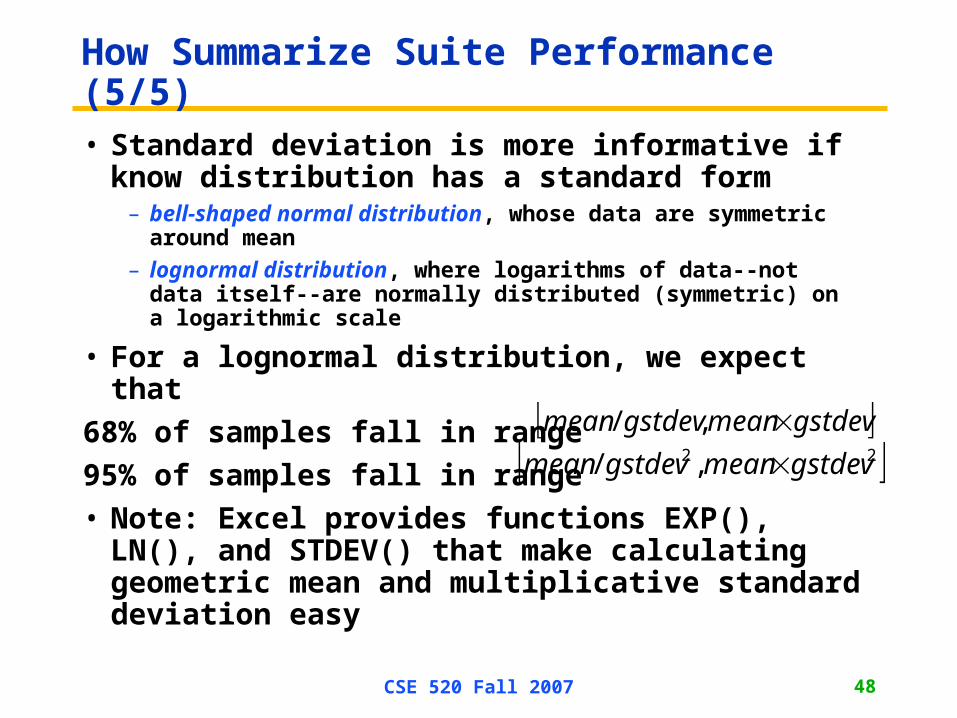
How Summarize Suite Performance (5/5)
• Standard deviation is more informative if know distribution has a standard form
– bell-shaped normal distribution, whose data are symmetric around mean
– lognormal distribution, where logarithms of data--not data itself--are normally distributed (symmetric) on a logarithmic scale
• For a lognormal distribution, we expect that
68% of samples fall in range
95% of samples fall in range
• Note: Excel provides functions EXP(), LN(), and STDEV() that make calculating geometric mean and multiplicative standard deviation easy
gstdevmeangstdevmean ,/
22 ,/ gstdevmeangstdevmean
CSE 520 Fall 2007 49
0
2000
4000
6000
8000
10000
12000
14000
wup
wis
e
swim
mgr
id
appl
u
mes
a
galg
el art
equa
ke
face
rec
amm
p
luca
s
fma3
d
sixt
rack
apsi
SP
EC
fpR
atio
1372
5362
2712
GM = 2712GSTEV = 1.98
Example Standard Deviation (1/2)
• GM and multiplicative StDev of SPECfp2000 for Itanium 2
CSE 520 Fall 2007 50
Example Standard Deviation (2/2)
• GM and multiplicative StDev of SPECfp2000 for AMD Athlon
0
2000
4000
6000
8000
10000
12000
14000
wup
wis
e
swim
mgr
id
appl
u
mes
a
galg
el art
equa
ke
face
rec
amm
p
luca
s
fma3
d
sixt
rack
apsi
SP
EC
fpR
atio
1494
29112086
GM = 2086GSTEV = 1.40
CSE 520 Fall 2007 51
Comments on Itanium 2 and Athlon
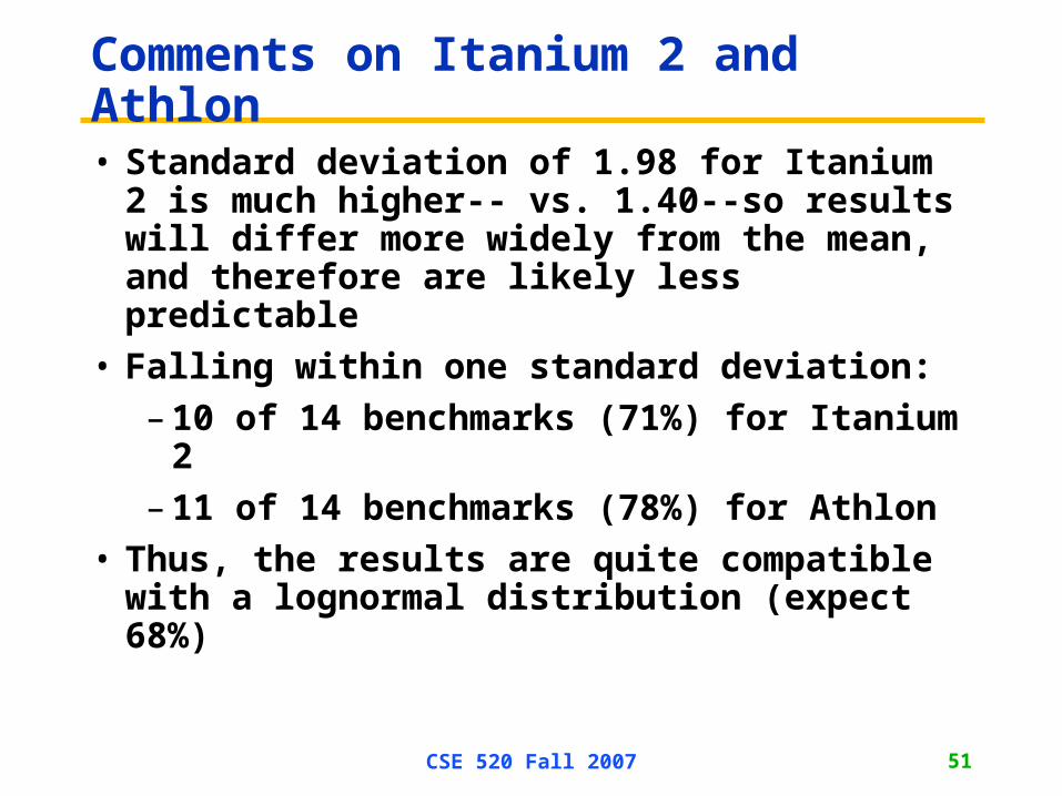
• Standard deviation of 1.98 for Itanium 2 is much higher-- vs. 1.40--so results will differ more widely from the mean, and therefore are likely less predictable
• Falling within one standard deviation:
– 10 of 14 benchmarks (71%) for Itanium 2
– 11 of 14 benchmarks (78%) for Athlon
• Thus, the results are quite compatible with a lognormal distribution (expect 68%)
CSE 520 Fall 2007 52
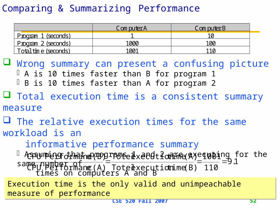
Comparing & Summarizing Performance
Computer A Computer BProgram 1 (seconds) 1 10Program 2 (seconds) 1000 100Total time (seconds) 1001 110
Wrong summary can present a confusing picture A is 10 times faster than B for program 1 B is 10 times faster than A for program 2
Total execution time is a consistent summary measure The relative execution times for the same workload is an informative performance summary
Assuming that programs 1 and 2 are executing for the same number of times on computers A and B
191101001
(B) time execution Totel(A) time execution Totel
(A) ePerformanc CPU(B) ePerformanc CPU
.
Execution time is the only valid and unimpeachable measure of performanceExecution time is the only valid and unimpeachable measure of performance
CSE 520 Fall 2007 53
Performance Reports
HardwareModel number Powerstation 550CPU 41.67-MHz POWER 4164FPU (floating point) IntegratedNumber of CPU 1Cache size per CPU 64K data/8k instructionMemory 64 MBDisk subsystem 2 400-MB SCSINetwork interface N/A
SoftwareOS type and revision AIX Ver. 3.1.5Compiler revision AIX XL C/6000 Ver. 1.1.5
AIX XL Fortran Ver. 2.2Other software NoneFile system type AIXFirmware level N/A
SystemTuning parameters NoneBackground load NoneSystem state Multi-user (single-user login)
Guiding principle is reproducibility (report environment & experiments setup)Guiding principle is reproducibility (report environment & experiments setup)
CSE 520 Fall 2007 54
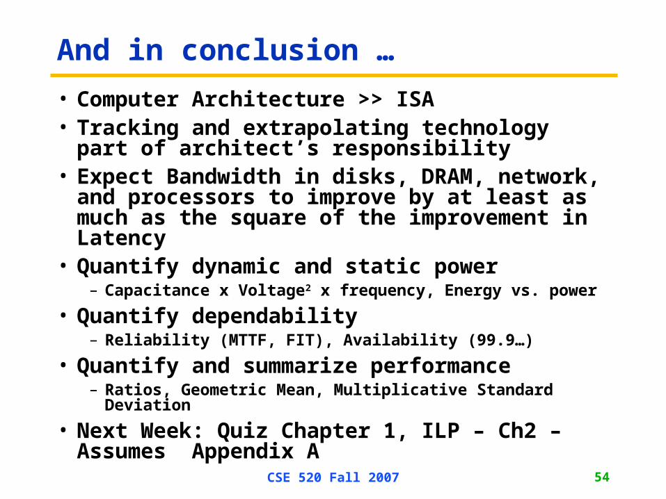
And in conclusion …
• Computer Architecture >> ISA• Tracking and extrapolating technology part of
architect’s responsibility• Expect Bandwidth in disks, DRAM, network, and
processors to improve by at least as much as the square of the improvement in Latency
• Quantify dynamic and static power– Capacitance x Voltage2 x frequency, Energy vs. power