39
CSE 781 Anti-aliasing for Texture Mapping
| Date post: | 14-Dec-2015 |
| Category: |
Documents |
| Upload: | lizeth-dorton |
| View: | 217 times |
| Download: | 2 times |

CSE 781
Anti-aliasing for Texture Mapping

Quality considerations
• So far we just mapped one point– results in bad aliasing (resampling problems)
• We really need to integrate over polygon• Super-sampling is not a very good solution– Dependent on area of integration.– Can be quit large for texture maps.
• Most popular (easiest) - mipmaps

Quality considerations
• Pixel area maps to “weird” (warped) shape in texture space
pixel
u
v
xs
ys

Quality Considerations
• We need to:– Calculate (or approximate) the integral of the
texture function under this area– Approximate:• Convolve with a wide filter around the center of this
area• Calculate the integral for a similar (but simpler) area.

Quality Considerations
• The area is typically approximated by a rectangular region (found to be good enough for most applications)
• Filter is typically a box/averaging filter - other possibilities
• How can we pre-compute this?

Mip-maps
• Mipmapping was invented in 1983 by Lance Williams– Multi in parvo “many things in a small place”

Mip-maps
• An image-pyramid is built.
256 pixels 128 64 32 16 8 4 2 1
Note: This only requires an additional 1/3 amount of texture
memory:1/4 + 1/16 + 1/64 +…

Mip-maps
• Find level of the mip-map where the area of each mip-map pixel is closest to the area of the mapped pixel.
pixel
u
v
xs
ys
2ix2i pixel level selected

Mip-maps
• Mip-maps are thus indexed by u, v, and the level, or amount of compression, d.
• The compression amount, d, will change according to the compression of the texels to the pixels, and for mip-maps can be approximated by:– d = sqrt( Area of pixel in uv-space )– The sqrt is due to the assumption of uniform compression
in mip-maps.

Review: Polygon Area
• Recall how to calculate the area of a 2D polygon (in this case, the quadrilateral of the mapped pixel corners).
A =
1
0112
1n
iiiii yxyx

Mip-maps
• William’s algorithm– Take the difference between neighboring u and v
coordinates to approximate derivatives across a screen step in x or y
– Derive a mipmap level from them by taking the maximum distortion• Over-blurring
2222 ,max yyxx vuvud d2log

Mip-maps
• The texel location can be determined to be either:1. The uv-mapping of the pixel center.2. The average u and v values from the projected pixel
corners (the centroid).3. The diagonal crossing of the projected
quadrilateral.
• However, there are only so many mip-map centers.
1
2
3

Mip-maps
• Pros– Easy to calculate:• Calculate pixels area in texture space• Determine mip-map level• Sample or interpolate to get color
• Cons– Area not very close – restricted to square shapes
(64x64 is far away from 128x128). – Location of area is not very tight - shifted.

Note on Alpha
• Alpha can be averaged just like rgb for texels
• Watch out for borders though if you interpolate

Specifying Mip-map levels• OpenGL allows you to specify each level individually
(see glTexImage2D function).• The GLU routine gluBuild2Dmipmaps() routine offers
an easy interface to averaging the original image down into its mip-map levels.
• You can (and probably should) recalculate the texture for each level.
Warning: By default, the filtering assumes mip-mapping. If you do not specify all of the mip-map levels, your image will probably be black.

Higher-levels of the Mip-map
• Two considerations should be made in the construction of the higher-levels of the mip-map.
1. Filtering – simple averaging using a box filter, apply a better low-pass filter.
2. Gamma correction – by taking into account the perceived brightness, you can maintain a more consistent effect as the object moves further away.

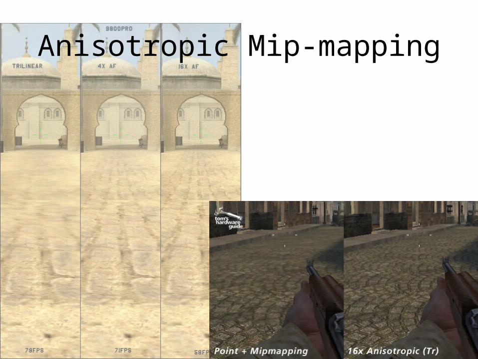
Anisotropic Filtering
• A pixel may rarely project onto texture space affinely.
• There may be large distortions in one direction.
isotropic

Anisotropic Filtering
• Multiple mip-maps or Ripmaps• Summed Area Tables (SAT)• Multi-sampling for anisotropic texture
filtering.• EWA filter

Ripmaps
• Scale by half by x across a row.
• Scale by half in y going down a column.
• The diagonal has the equivalent mip-map.
• Four times the amount of storage is required.

Ripmaps
• To use a ripmap, we use the pixel’s extents to determine the appropriate compression ratios.
• This gives us the four neighboring maps from which to sample and interpolate from.

Ripmaps
Compression in u is 1.7Compression in v is 6.8
Determine weights from each sample
pixel
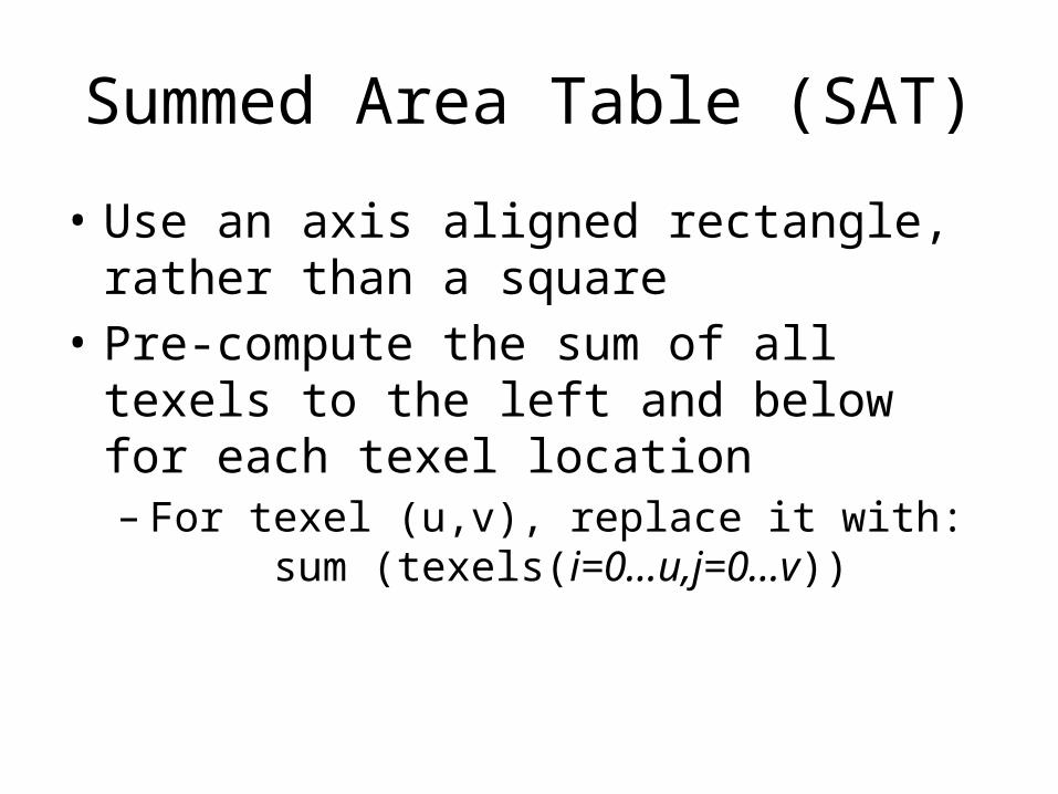
Summed Area Table (SAT)
• Use an axis aligned rectangle, rather than a square
• Pre-compute the sum of all texels to the left and below for each texel location– For texel (u,v), replace it with:
sum (texels(i=0…u,j=0…v))

Summed Area Table (SAT)
• Determining the rectangle:– Find bounding box and calculate its aspect ratio
pixel
u
v
xs
ys

Summed Area Table (SAT)
• Determine the rectangle with the same aspect ratio as the bounding box and the same area as the pixel mapping.
pixel
u
v
xs
ys

Summed Area Table (SAT)
• Center this rectangle around the bounding box center.
• Formula:• Area = aspect_ratio*x*x• Solve for x – the width of the rectangle
• Other derivations are also possible using the aspects of the diagonals, …

Summed Area Table (SAT)
• Calculating the color– We want the average of the texel colors within this
rectangle
u
v+
+ -
-
(u3,v3)
(u2,v2)(u1,v1)
(u4,v4)
+ -
+-

Summed Area Table (SAT)
• To get the average, we need to divide by the number of texels falling in the rectangle.– Color = SAT(u3,v3)-SAT(u4,v4)-SAT(u2,v2)+SAT(u1,v1)– Color = Color / ( (u3-u1)*(v3-v1) )
• This implies that the values for each texel may be very large:– For 8-bit colors, we could have a maximum SAT value of 255*nx*ny– 32-bit integers would handle a 4kx4k texture with 8-bit values.– RGB images imply 12-bytes per pixel.

Summed Area Table (SAT)
• Pros– Still relatively simple
• Calculate four corners of rectangle• 4 look-ups, 5 additions, 1 multiply and 1 divide.
– Better fit to area shape– Better overlap
• Cons– Large texel SAT values needed.– Still not a perfect fit to the mapped pixel.– The divide is expensive in hardware.

Anisotropic Mip-mapping
• Uses parallel hardware to obtain multiple mip-map samples for a fragment.
• A lower-level (higher-res level) of the mip-map is used.
• Calculate d as the minimumlength, ratherthan themaximum.
Anisotropic Mip-mapping

Anisotropic Mip-mapping

Elliptical Weighted Average (EWA) Filter
• Treat each pixel as circular, rather than square.• Mapping of a circle is elliptical in texel space.
pixel
u
v
xs
ys
The gold standard. Used to compare all
other techniques
against.

EWA Filter
• Precompute?• Can use a better filter than a box filter. • Heckbert chooses a Gaussian filter.

EWA Filter
• Calculating the Ellipse• Scan converting the Ellipse• Determining the final color (normalizing the
value or dividing by the weighted area).

EWA Filter
• Calculating the ellipse– We have a circular function defined in (x,y).– Filtering that in texture space h(u,v).– (u,v) = T(x,y)– Filter: h(T(x,y))

EWA Filter
• Ellipse:– (u,v) = Au2 + Buv + Cv2 = F– (u,v) = (0,0) at center of the ellipse• A = vx
2 +vy2
• B = -2(uxvy + uyvx)
• C = ux2 +uy
2
• F = uxvy + uyvx

EWA Filter
• Scan converting the ellipse:– Determine the bounding box– Scan convert the pixels within it, calculating (u,v).– If (u,v) < F, weight the underlying texture value by
the filter kernel and add to the sum.– Also, sum up the filter kernel values within the
ellipse.

EWA Filter
• Determining the final color– Divide the weighted sum of texture values by the
sum of the filter weights.

EWA Filter
• What about large areas?– If m pixels fall within the bounding box of the ellipse, then
we have O(n2m) algorithm for an nxn image.– m maybe rather large.
• We can apply this on a mip-map pyramid,rather than the full detailed image.– Tighter-fit of the mapped pixel– Cross between a box filter and gaussian filter.– Constant complexity - O(n2)


