84
CSE241 L8 Placement.1 Kahng & Cichy, UCSD ©2003 CSE241 CSE241 VLSI Digital Circuits VLSI Digital Circuits Winter 2003 Winter 2003 Lecture 08: Placement Lecture 08: Placement
| Date post: | 21-Dec-2015 |
| Category: |
Documents |
| View: | 219 times |
| Download: | 0 times |
CSE241 L8 Placement.1 Kahng & Cichy, UCSD ©2003
CSE241CSE241VLSI Digital CircuitsVLSI Digital Circuits
Winter 2003Winter 2003
Lecture 08: PlacementLecture 08: Placement
CSE241 L8 Placement.2 Kahng & Cichy, UCSD ©2003
IntroductionIntroductionIntroductionIntroduction
Dr. Gabriel Robins [email protected] www.cs.virginia.edu/robins
Dr. Gabriel Robins [email protected] www.cs.virginia.edu/robins
CSE241 L8 Placement.3 Kahng & Cichy, UCSD ©2003
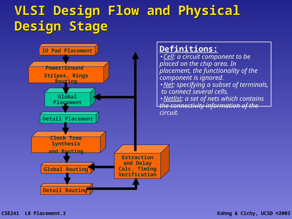
VLSI Design Flow and Physical Design VLSI Design Flow and Physical Design StageStageVLSI Design Flow and Physical Design VLSI Design Flow and Physical Design StageStage
Definitions:•Cell: a circuit component to be placed on the chip area. In placement, the functionality of the component is ignored.•Net: specifying a subset of terminals, to connect several cells.•Netlist: a set of nets which contains the connectivity information of the circuit.Global
Placement
Detail Placement
Clock Tree Synthesis
and Routing
Global Routing
Detail Routing
Power/Ground
Stripes, Rings Routing
Extraction and Delay Calc.
Timing Verification
IO Pad Placement
CSE241 L8 Placement.4 Kahng & Cichy, UCSD ©2003
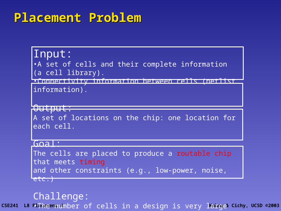
Placement ProblemPlacement ProblemPlacement ProblemPlacement Problem
Input:•A set of cells and their complete information (a cell library).•Connectivity information between cells (netlist information).
Output: A set of locations on the chip: one location for each cell.
Goal:The cells are placed to produce a routable chip that meets timing and other constraints (e.g., low-power, noise, etc.)
Challenge:•The number of cells in a design is very large (> 1 million).•The timing constraints are very tight.
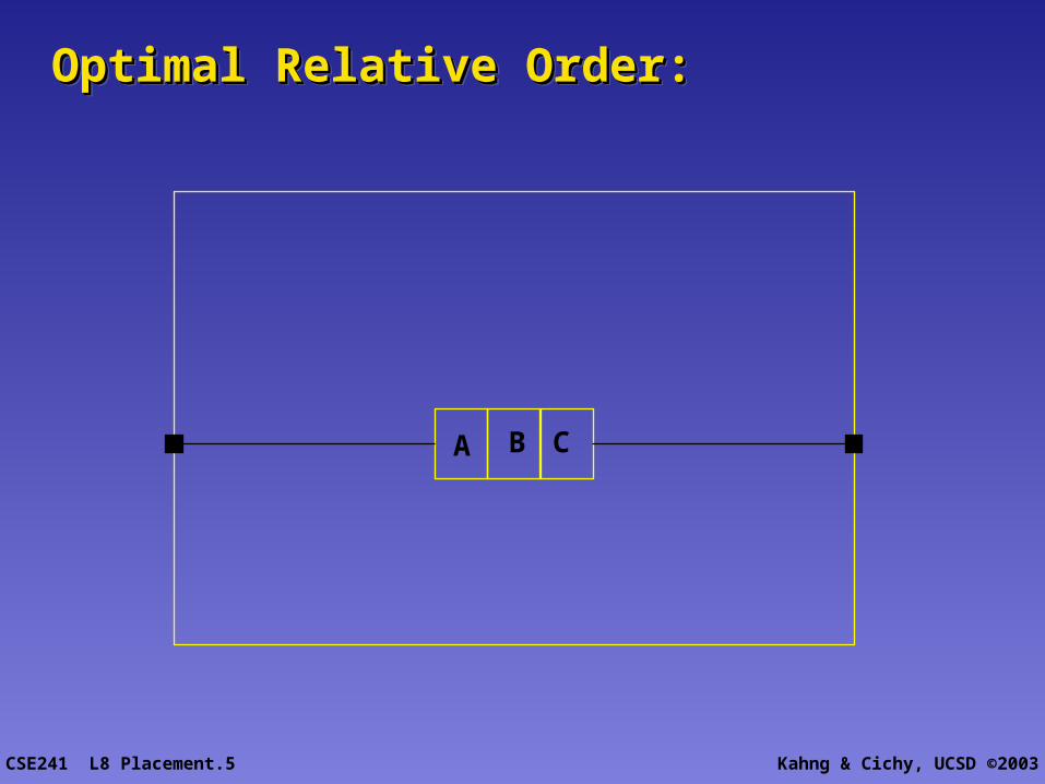
CSE241 L8 Placement.5 Kahng & Cichy, UCSD ©2003
A B C
Optimal Relative Order:Optimal Relative Order:Optimal Relative Order:Optimal Relative Order:
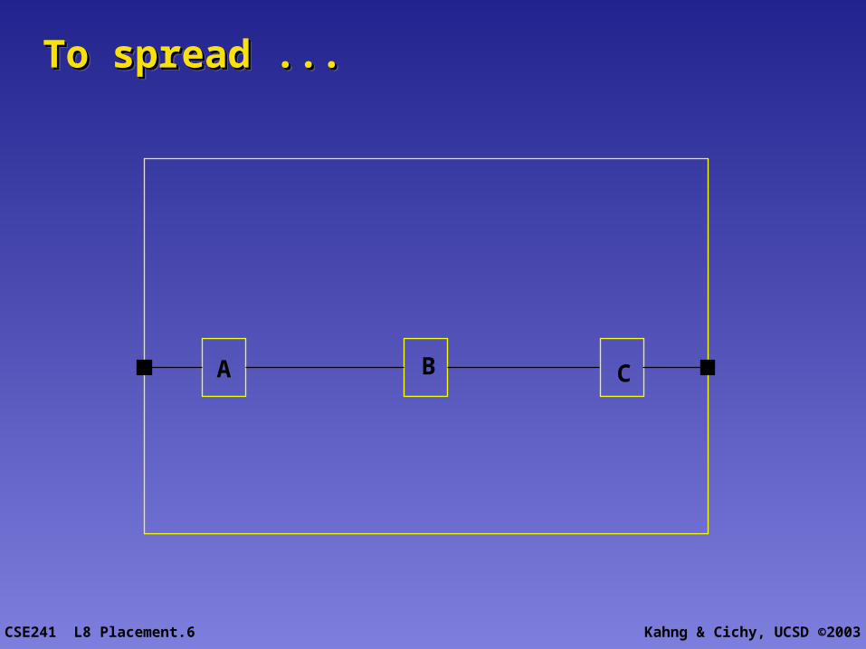
CSE241 L8 Placement.6 Kahng & Cichy, UCSD ©2003
A B C
To spread ...To spread ...To spread ...To spread ...
CSE241 L8 Placement.7 Kahng & Cichy, UCSD ©2003
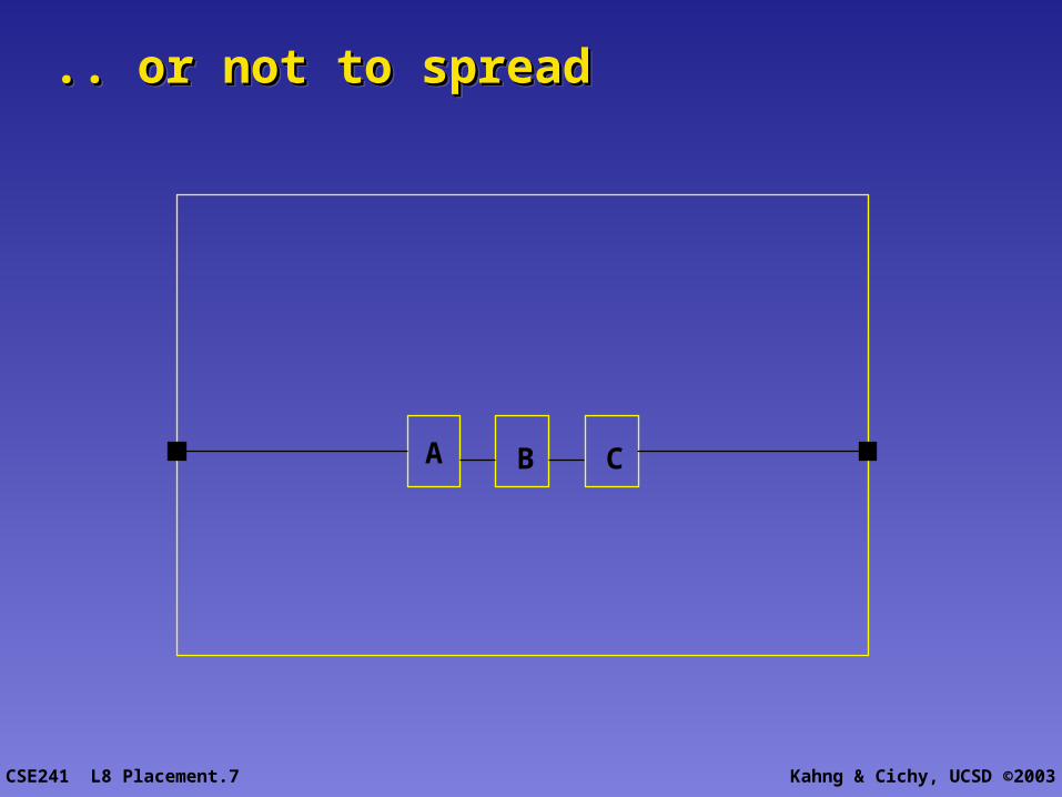
A B C
.. or not to spread.. or not to spread.. or not to spread.. or not to spread
CSE241 L8 Placement.8 Kahng & Cichy, UCSD ©2003
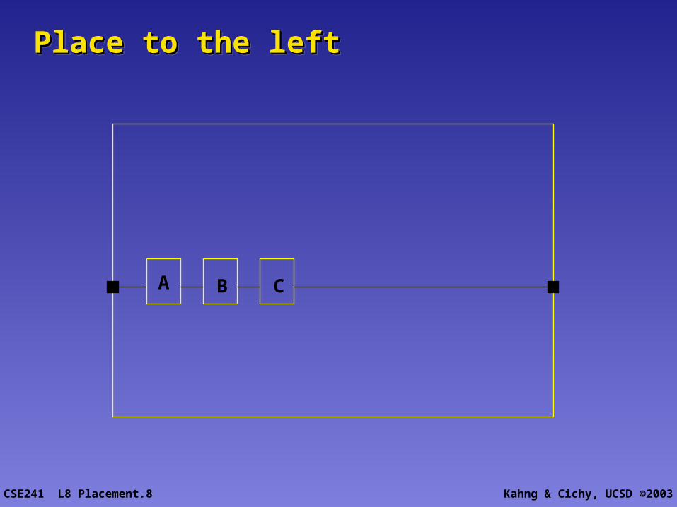
A B C
Place to the leftPlace to the leftPlace to the leftPlace to the left
CSE241 L8 Placement.9 Kahng & Cichy, UCSD ©2003
A B C
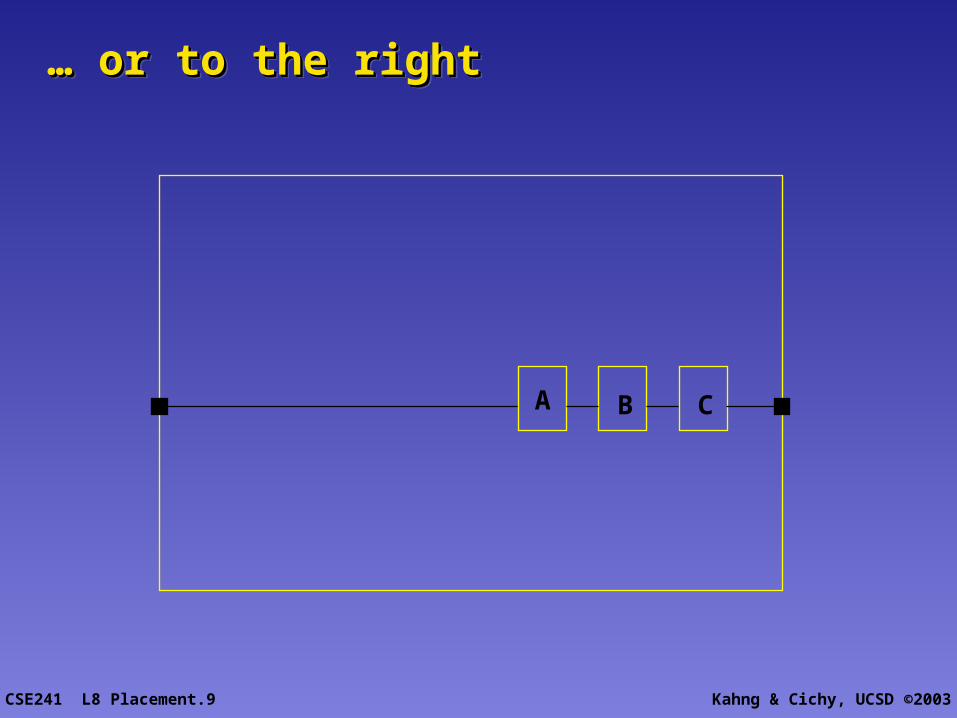
… … or to the rightor to the right… … or to the rightor to the right
CSE241 L8 Placement.10 Kahng & Cichy, UCSD ©2003
A B C
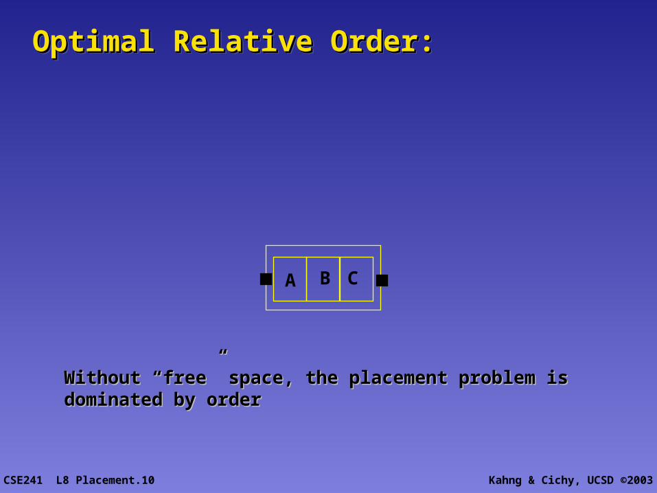
Optimal Relative Order:Optimal Relative Order:Optimal Relative Order:Optimal Relative Order:
Without “free” space, the placement problem is dominated by Without “free” space, the placement problem is dominated by orderorder
CSE241 L8 Placement.11 Kahng & Cichy, UCSD ©2003
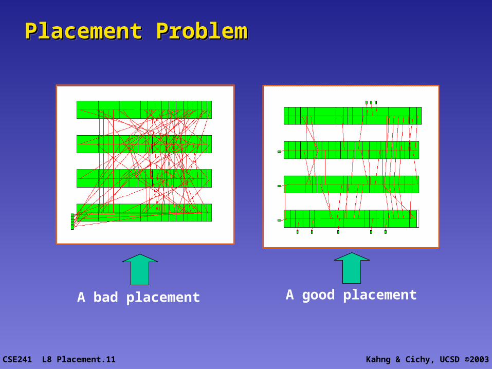
Placement ProblemPlacement ProblemPlacement ProblemPlacement Problem
A bad placement A good placement
CSE241 L8 Placement.12 Kahng & Cichy, UCSD ©2003
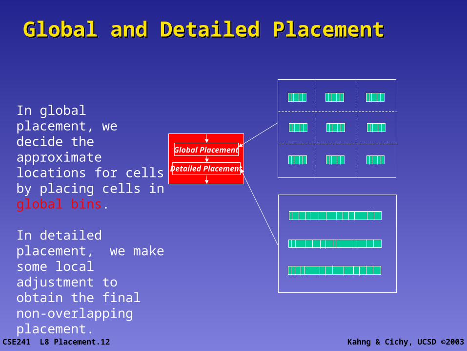
Global and Detailed PlacementGlobal and Detailed PlacementGlobal and Detailed PlacementGlobal and Detailed Placement
Global Placement
Detailed Placement
In global placement, we decide the approximate locations for cells by placing cells in global bins.
In detailed placement, we make some local adjustment to obtain the final non-overlapping placement.
CSE241 L8 Placement.13 Kahng & Cichy, UCSD ©2003
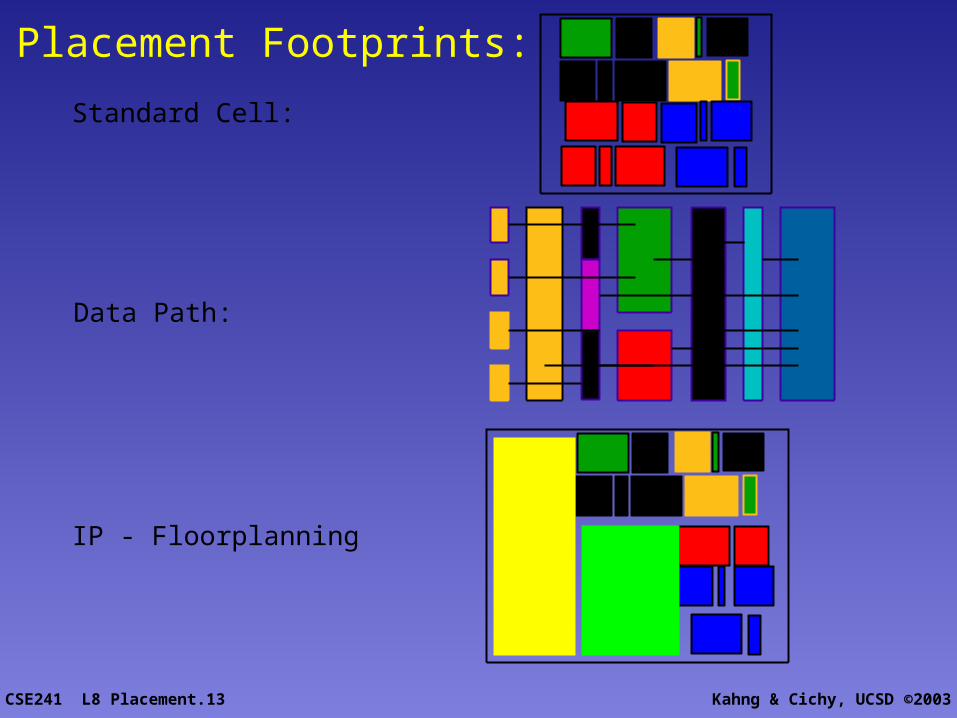
Placement Footprints:
Standard Cell:
Data Path:
IP - Floorplanning
CSE241 L8 Placement.14 Kahng & Cichy, UCSD ©2003
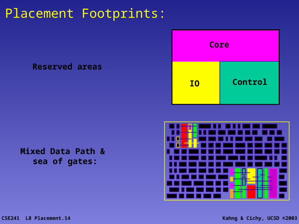
Core
ControlIO
Reserved areas
Mixed Data Path & sea of gates:
Placement Footprints:
CSE241 L8 Placement.15 Kahng & Cichy, UCSD ©2003
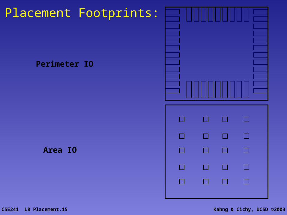
Perimeter IO
Area IO
Placement Footprints:

CSE241 L8 Placement.16 Kahng & Cichy, UCSD ©2003
Placement objectives are subject to user constraints / Placement objectives are subject to user constraints / design style:design style:Placement objectives are subject to user constraints / Placement objectives are subject to user constraints / design style:design style:
Hierarchical Design Constraints pin location power rail reserved layers
Flat Design with Floorplan Constraints Fixed Circuits I/O Connections
Hierarchical Design Constraints pin location power rail reserved layers
Flat Design with Floorplan Constraints Fixed Circuits I/O Connections
CSE241 L8 Placement.17 Kahng & Cichy, UCSD ©2003
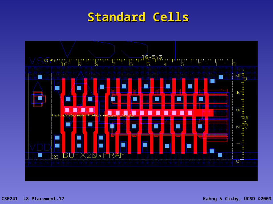
Standard CellsStandard CellsStandard CellsStandard Cells
CSE241 L8 Placement.18 Kahng & Cichy, UCSD ©2003
Standard CellsStandard CellsStandard CellsStandard Cells
Power connected by abutment, placed in sea-of-rows Rarely rotated DRC clean in any combination Circuit clean (I.e. no naked T-gates, no huge input
capacitances) 8,9,10+ tracks in height Metal 1 only used (hopefully) Multi-height stdcells possible Buffers: sizes, intrinsic delay steps, optimal repeater selection Special clock buffers + gates (balanced P:N) Special metastability hardened flops Cap cells (metal1 used?) Gap fillers (metal1 used?) Tie-high, tie-low
CSE241 L8 Placement.19 Kahng & Cichy, UCSD ©2003
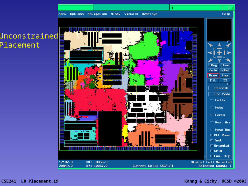
UnconstrainedPlacement
CSE241 L8 Placement.20 Kahng & Cichy, UCSD ©2003
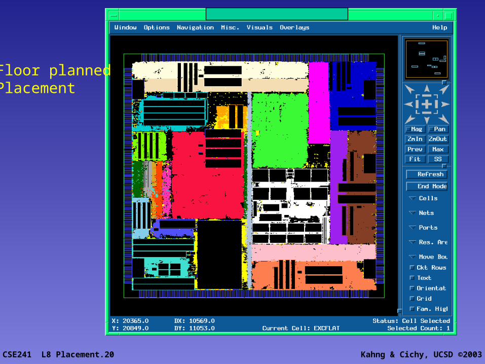
Floor plannedPlacement
CSE241 L8 Placement.21 Kahng & Cichy, UCSD ©2003
Placement Cube Placement Cube (4D)(4D) Placement Cube Placement Cube (4D)(4D)
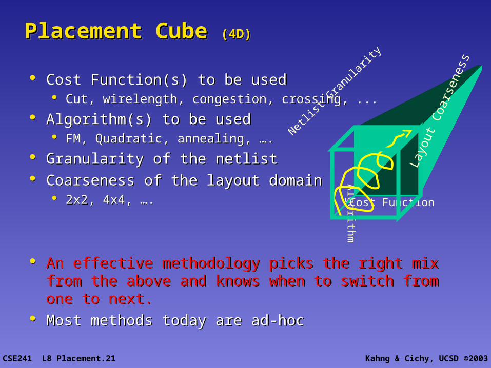
Cost Function(s) to be used Cut, wirelength, congestion, crossing, ...
Algorithm(s) to be used FM, Quadratic, annealing, ….
Granularity of the netlist Coarseness of the layout domain
2x2, 4x4, ….
An effective methodology picks the right mix from the above and knows when to switch from one to next.
Most methods today are ad-hoc
Algorithm
Cost Function
Netlist
Gran
ularit
y
Layo
ut C
oars
enes
s
CSE241 L8 Placement.22 Kahng & Cichy, UCSD ©2003
Advantages of HierarchyAdvantages of HierarchyAdvantages of HierarchyAdvantages of Hierarchy
Design is carved into smaller pieces that can be worked on in parallel (improved throughput)
A known floor plan provides the logic design team with a large degree of placement control.
A known floor plan provided early knowledge of long wires Timing closure problems can be addressed by tools, logic design, and
hierarchy manipulation Late design changes can be done with minimal turmoil to the entire design
CSE241 L8 Placement.23 Kahng & Cichy, UCSD ©2003
Disadvantages of HierarchyDisadvantages of HierarchyDisadvantages of HierarchyDisadvantages of Hierarchy
Results depend on the quality of the hierarchy. The logic hierarchy must be designed with PD taken into account.
Additional methodology requirements must be met to enable hierarchy. Ex. Pin assignment, Macro Abstract management, area budgeting, floor planning, timing budgets, etc
Late design changes may affect multiple components. Hierarchy allows divergent methodologies Hierarchy hinders DA algorithms. They can no longer perform global
optimizations.
CSE241 L8 Placement.24 Kahng & Cichy, UCSD ©2003
Traditional Placement AlgorithmsTraditional Placement AlgorithmsTraditional Placement AlgorithmsTraditional Placement Algorithms
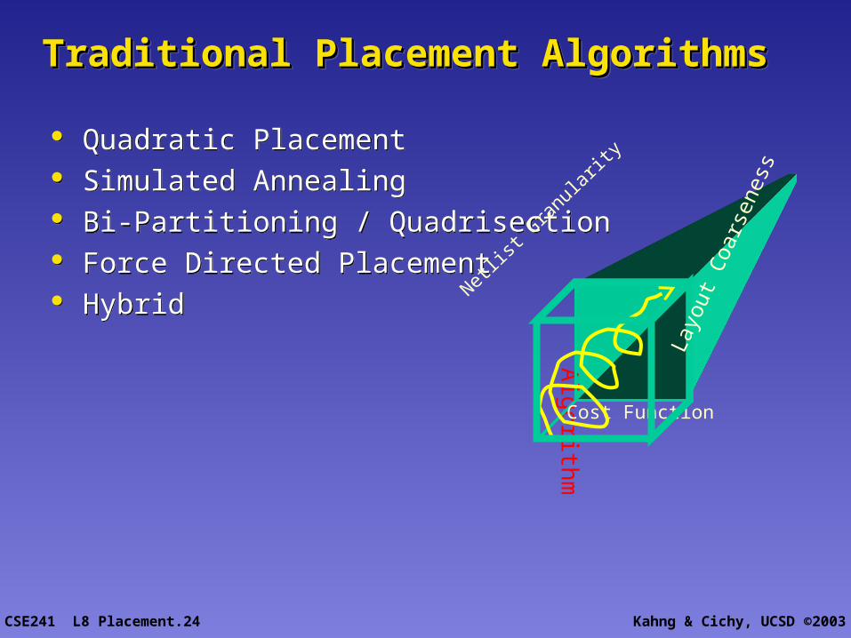
Quadratic Placement Simulated Annealing Bi-Partitioning / Quadrisection Force Directed Placement Hybrid
Quadratic Placement Simulated Annealing Bi-Partitioning / Quadrisection Force Directed Placement Hybrid
Algorithm
Cost Function
Netlist
Gran
ularit
y
Layo
ut C
oars
enes
s
CSE241 L8 Placement.25 Kahng & Cichy, UCSD ©2003
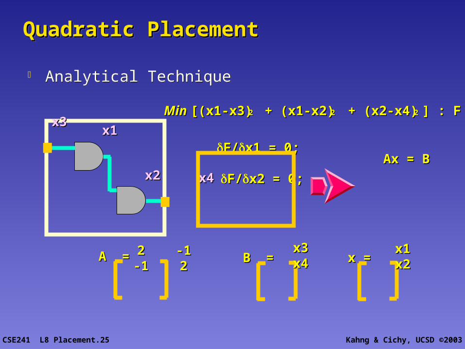
Quadratic PlacementQuadratic PlacementQuadratic PlacementQuadratic Placement
Analytical Technique Analytical Technique
x4x4
x3x3x1x1
x2x2
Min Min [(x1-x3)[(x1-x3)22 + (x1-x2) + (x1-x2)2 2 + (x2-x4)+ (x2-x4)22 ] : ] : FF
F/F/x1 = 0; x1 = 0;
F/F/x2 = 0;x2 = 0;
Ax = BAx = B
2 -12 -1-1 2-1 2
x = x = x1x1x2x2
A = A = B = B = x3x3x4x4
CSE241 L8 Placement.26 Kahng & Cichy, UCSD ©2003
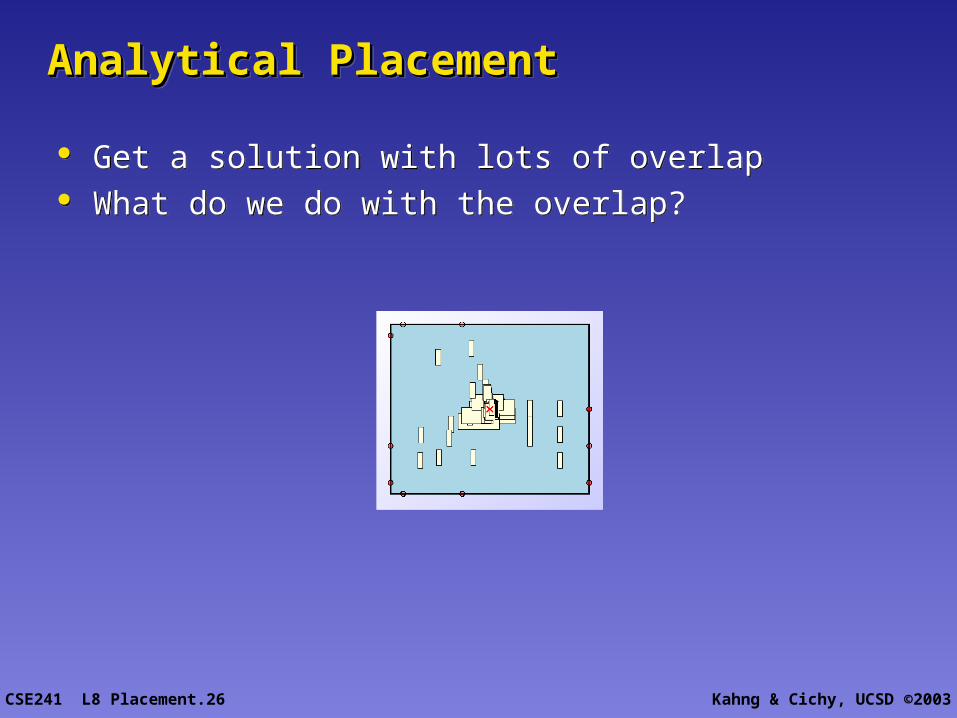
Analytical PlacementAnalytical PlacementAnalytical PlacementAnalytical Placement
Get a solution with lots of overlap What do we do with the overlap?
Get a solution with lots of overlap What do we do with the overlap?
CSE241 L8 Placement.27 Kahng & Cichy, UCSD ©2003
Pros and Cons of QPPros and Cons of QPPros and Cons of QPPros and Cons of QP
Pros: Very Fast Analytical Solution Can Handle Large Design Sizes Can be Used as an Initial Seed Placement Engine
Cons: Can Generate Overlapped Solutions: Postprocessing Needed Not Suitable for Timing Driven Placement Not Suitable for Simultaneous Optimization of Other Aspects of
Physical Design (clocks, crosstalk…) Gives Trivial Solutions without Pads (and close to trivial with
pads)
CSE241 L8 Placement.28 Kahng & Cichy, UCSD ©2003
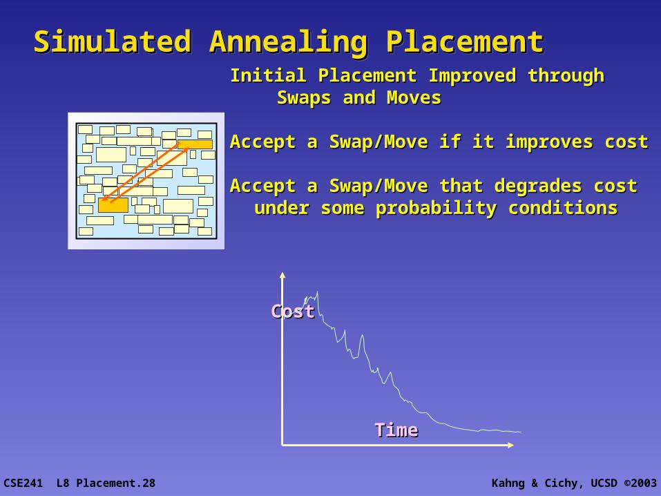
Simulated Annealing PlacementSimulated Annealing PlacementSimulated Annealing PlacementSimulated Annealing Placement Initial Placement Improved throughInitial Placement Improved through Swaps and MovesSwaps and Moves
Accept a Swap/Move if it improves costAccept a Swap/Move if it improves cost
Accept a Swap/Move that degrades costAccept a Swap/Move that degrades costunder some probability conditionsunder some probability conditions
TimeTime
CostCost
CSE241 L8 Placement.29 Kahng & Cichy, UCSD ©2003
Pros and Cons of SA Pros and Cons of SA Pros and Cons of SA Pros and Cons of SA
Pros: Can Reach Globally Optimal Solution (given “enough” time) Open Cost Function. Can Optimize Simultaneously all Aspects of Physical Design Can be Used for End Case Placement
Cons: Extremely Slow Process of Reaching a Good Solution
Pros: Can Reach Globally Optimal Solution (given “enough” time) Open Cost Function. Can Optimize Simultaneously all Aspects of Physical Design Can be Used for End Case Placement
Cons: Extremely Slow Process of Reaching a Good Solution
CSE241 L8 Placement.30 Kahng & Cichy, UCSD ©2003
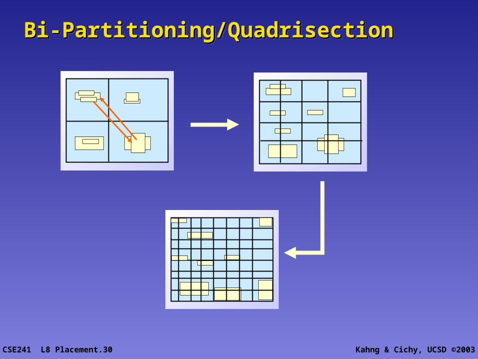
Bi-Partitioning/QuadrisectionBi-Partitioning/QuadrisectionBi-Partitioning/QuadrisectionBi-Partitioning/Quadrisection
CSE241 L8 Placement.31 Kahng & Cichy, UCSD ©2003
Pros and Cons of Partitioning Based Pros and Cons of Partitioning Based PlacementPlacementPros and Cons of Partitioning Based Pros and Cons of Partitioning Based PlacementPlacement
Pros: More Suitable to Timing Driven Placement since it is Move
Based New Innovation (hMetis) in Partitioning Algorithms have made
this Extremely Fast Open Cost Function Move Based means Simultaneous Optimization of all Design
Aspects Possible Cons:
Not Well Understood Lots of “indifferent” moves May not work well with some cost functions.
CSE241 L8 Placement.32 Kahng & Cichy, UCSD ©2003
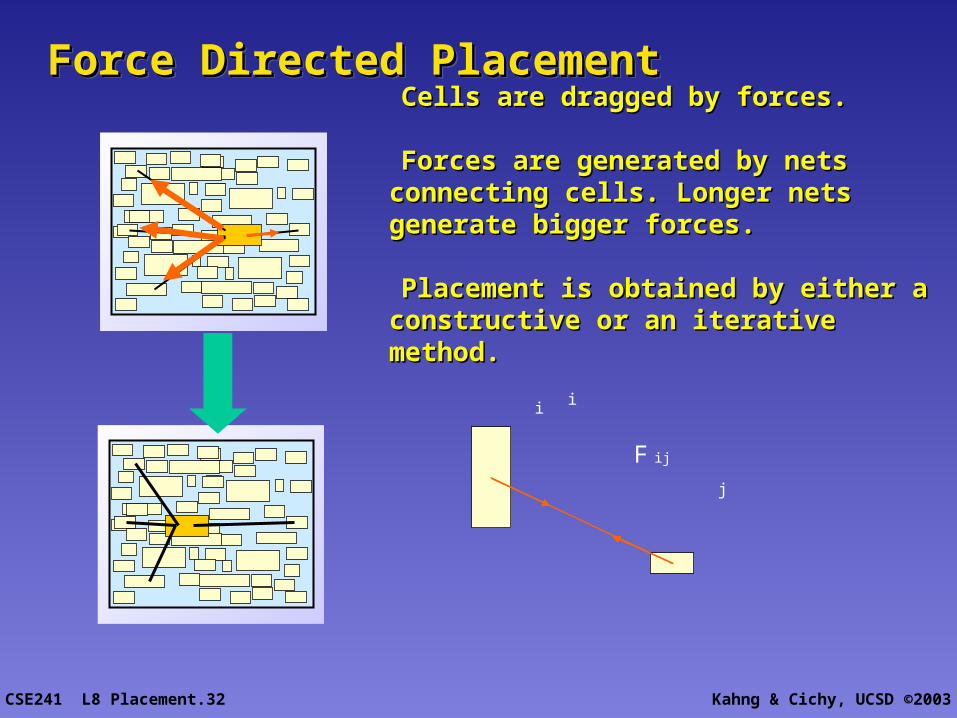
Force Directed PlacementForce Directed PlacementForce Directed PlacementForce Directed Placement
Cells are dragged by forces.Cells are dragged by forces.
Forces are generated by nets connecting cells. Forces are generated by nets connecting cells. Longer nets generate bigger forces.Longer nets generate bigger forces.
Placement is obtained by either a constructive Placement is obtained by either a constructive or an iterative method.or an iterative method.
i
j
F ij
i
CSE241 L8 Placement.33 Kahng & Cichy, UCSD ©2003
Pros and Cons of Force Directed Pros and Cons of Force Directed PlacementPlacementPros and Cons of Force Directed Pros and Cons of Force Directed PlacementPlacement
Pros: Very Fast Analytical Solution Can Handle Large Design Sizes Can be Used as an Initial Seed Placement Engine The Force
Cons: Not sensitive to the non-overlapping constraints Gives Trivial Solutions without Pads Not Suitable for Timing Driven Placement
Pros: Very Fast Analytical Solution Can Handle Large Design Sizes Can be Used as an Initial Seed Placement Engine The Force
Cons: Not sensitive to the non-overlapping constraints Gives Trivial Solutions without Pads Not Suitable for Timing Driven Placement
CSE241 L8 Placement.34 Kahng & Cichy, UCSD ©2003
Hybrid PlacementHybrid PlacementHybrid PlacementHybrid Placement
Mix-matching different placement algorithms Effective algorithms are always hybrid
Mix-matching different placement algorithms Effective algorithms are always hybrid
CSE241 L8 Placement.35 Kahng & Cichy, UCSD ©2003
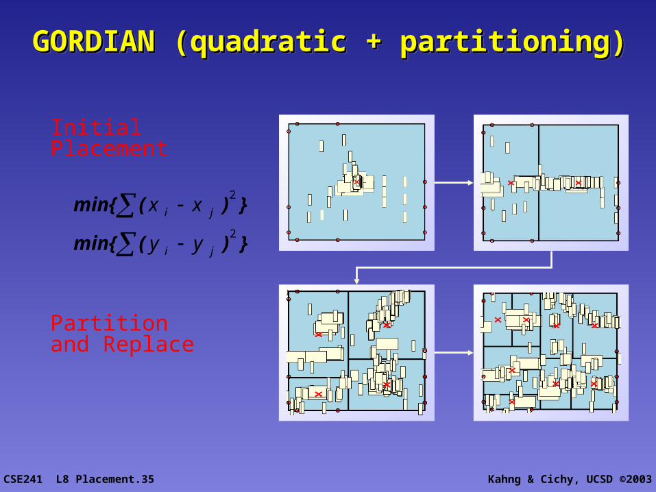
GORDIAN (quadratic + partitioning)GORDIAN (quadratic + partitioning)GORDIAN (quadratic + partitioning)GORDIAN (quadratic + partitioning)
Partitionand Replace
InitialPlacement
})(min{
})(min{2
2
ji
ji
yy
xx
CSE241 L8 Placement.36 Kahng & Cichy, UCSD ©2003
Congestion MinimizationCongestion MinimizationCongestion MinimizationCongestion Minimization
Traditional placement problem is to minimize interconnection length (wirelength)
A valid placement has to be routable Congestion is important because it represents
routability (lower congestion implies better routability)
There is not yet enough research work on the congestion minimization problem
Traditional placement problem is to minimize interconnection length (wirelength)
A valid placement has to be routable Congestion is important because it represents
routability (lower congestion implies better routability)
There is not yet enough research work on the congestion minimization problem
CSE241 L8 Placement.37 Kahng & Cichy, UCSD ©2003
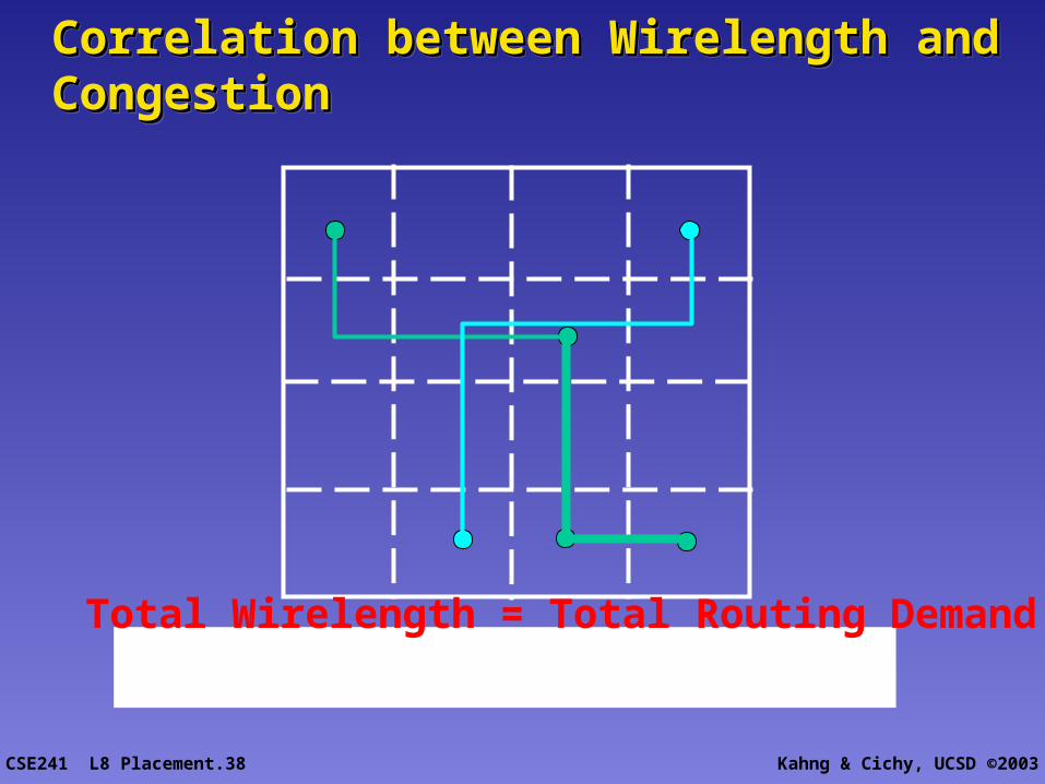
Definition of CongestionDefinition of CongestionDefinition of CongestionDefinition of Congestion
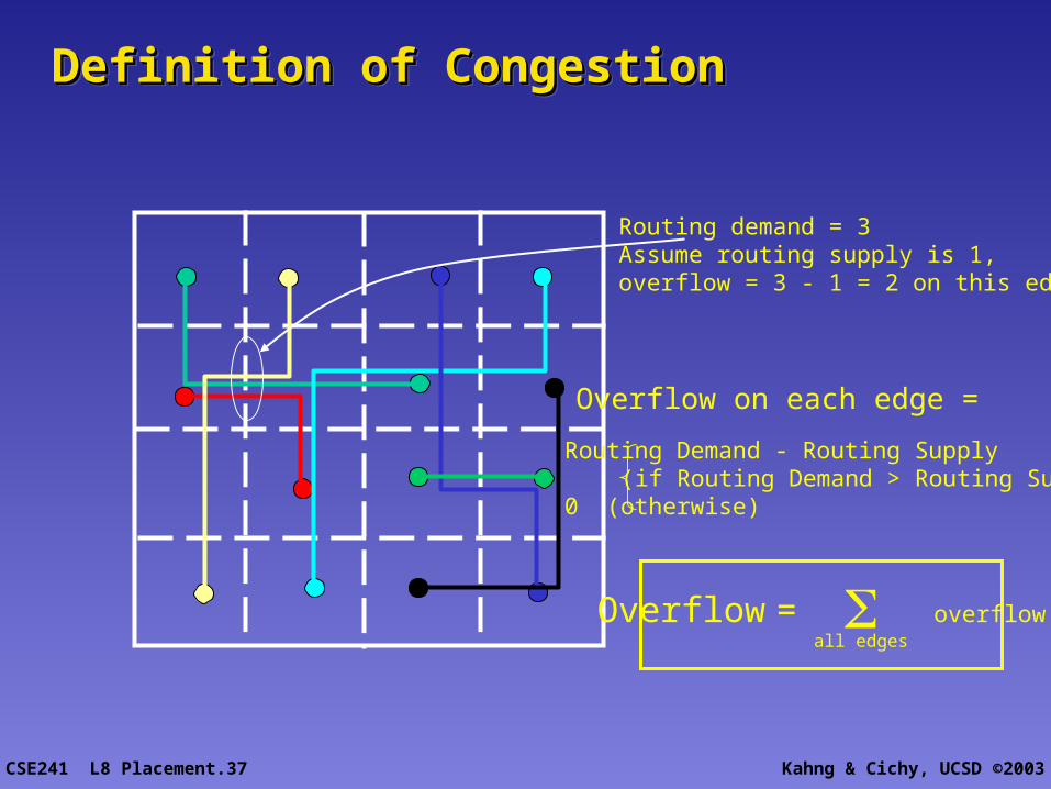
Routing demand = 3Assume routing supply is 1,overflow = 3 - 1 = 2 on this edge.
Overflow = overflowall edges
Overflow on each edge =
Routing Demand - Routing Supply (if Routing Demand > Routing Supply)0 (otherwise)
CSE241 L8 Placement.38 Kahng & Cichy, UCSD ©2003
Correlation between Wirelength and Correlation between Wirelength and CongestionCongestionCorrelation between Wirelength and Correlation between Wirelength and CongestionCongestion
Total Wirelength = Total Routing Demand
CSE241 L8 Placement.39 Kahng & Cichy, UCSD ©2003
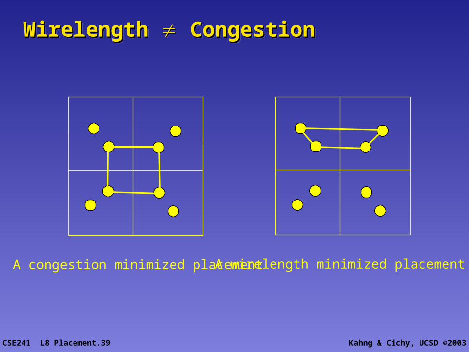
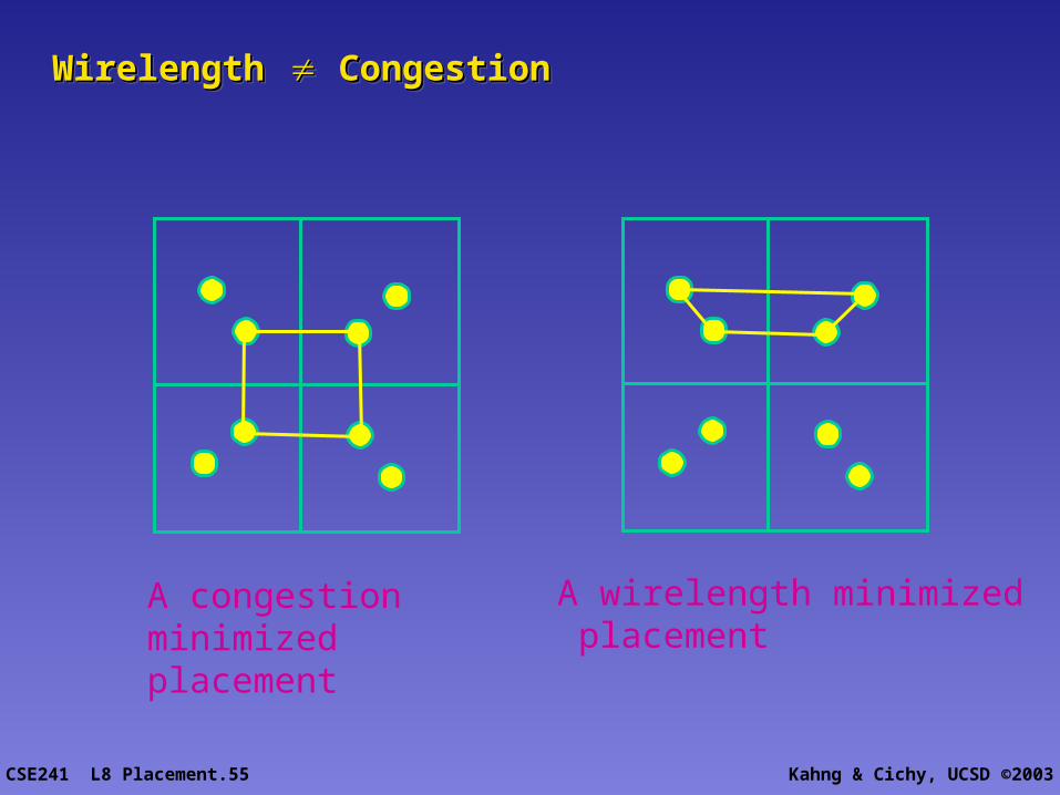
Wirelength Wirelength Congestion CongestionWirelength Wirelength Congestion Congestion
A congestion minimized placement A wirelength minimized placement

CSE241 L8 Placement.40 Kahng & Cichy, UCSD ©2003
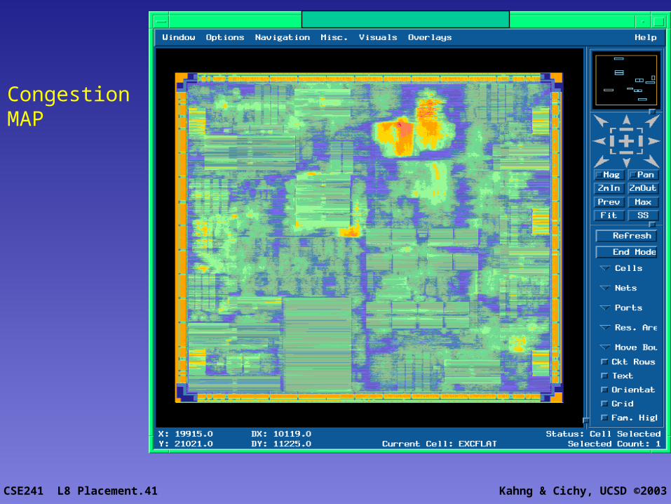
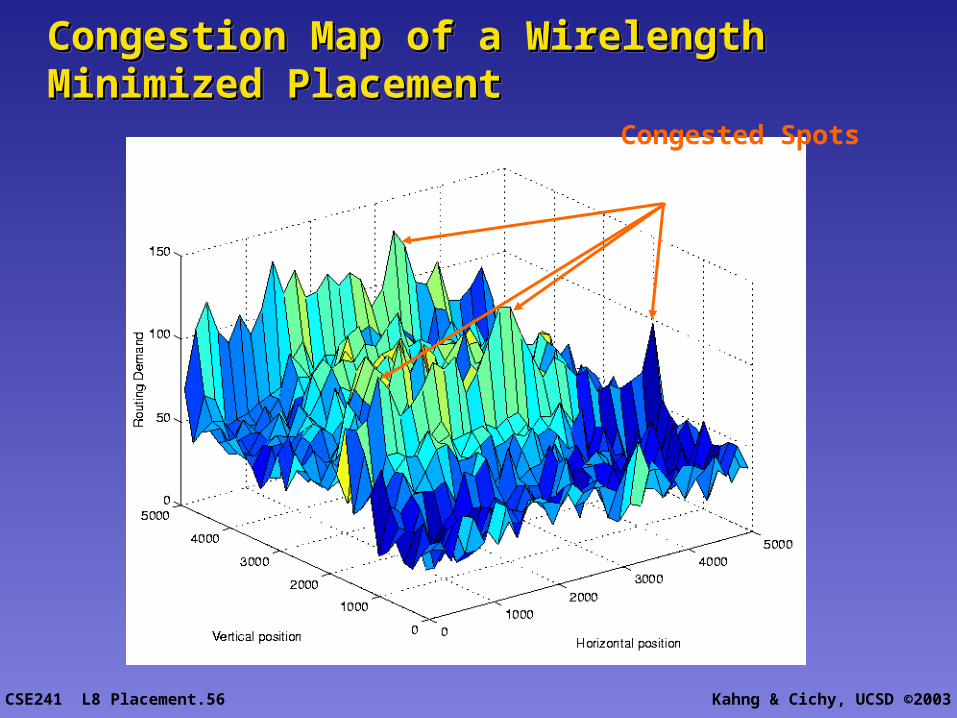
Congestion Map of a Wirelength Minimized Congestion Map of a Wirelength Minimized PlacementPlacementCongestion Map of a Wirelength Minimized Congestion Map of a Wirelength Minimized PlacementPlacement
Congested Spots
CSE241 L8 Placement.41 Kahng & Cichy, UCSD ©2003
CongestionMAP
CSE241 L8 Placement.42 Kahng & Cichy, UCSD ©2003
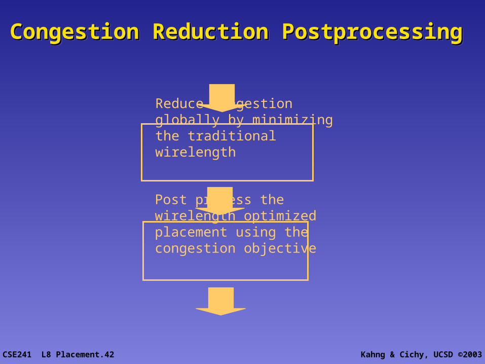
Congestion Reduction Postprocessing Congestion Reduction Postprocessing Congestion Reduction Postprocessing Congestion Reduction Postprocessing
Reduce congestion globally by minimizing the traditional wirelength
Post process the wirelength optimized placement using the congestion objective
CSE241 L8 Placement.43 Kahng & Cichy, UCSD ©2003
Among a variety of cost functions and methods for congestion minimization, wirelength alone followed by a post processing congestion minimization works the best and is one of the fastest.
Cost functions such as a hybrid length plus congestion do not work very well.
Among a variety of cost functions and methods for congestion minimization, wirelength alone followed by a post processing congestion minimization works the best and is one of the fastest.
Cost functions such as a hybrid length plus congestion do not work very well.
Congestion Reduction Postprocessing Congestion Reduction Postprocessing Congestion Reduction Postprocessing Congestion Reduction Postprocessing
CSE241 L8 Placement.44 Kahng & Cichy, UCSD ©2003
Cost Functions for PlacementCost Functions for PlacementCost Functions for PlacementCost Functions for Placement
The final goal of placement is to achieve routability and meet timing constraints
Constraints are very hard to use in optimization, thus we use cost functions (e.g., Wirelength) to predict our goals.
We will show what happens when you try constraints directly The main challenge is a technical understanding of various cost
functions and their interaction.
CSE241 L8 Placement.45 Kahng & Cichy, UCSD ©2003
Prediction
What is prediction ? every system has some critical cost functions: Area,
wirelength, congestion, timing etc. Prediction aims at estimating values of these cost
functions without having to go through the time-consuming process of full construction.
Allows quick space exploration, localizes the search
For example: statistical wire-load models Wirelength in placement
CSE241 L8 Placement.46 Kahng & Cichy, UCSD ©2003
Paradigms of Prediction Two fundamental paradigms
statistical prediction #of two-terminal nets in all designs #of two-terminal nets with length greater than 10 in all
designs constructive prediction
#of two-terminal nets with length greater than 10 in this design
… and everything in between, e.g., #of critical two-terminal nets in a design based on
statistical data and a quick inspection of the design in hand.
“Absolute truth” or “I need it to make progress” SLIP (System Level Interconnect Prediction)
community.
Two fundamental paradigms statistical prediction
#of two-terminal nets in all designs #of two-terminal nets with length greater than 10 in all
designs constructive prediction
#of two-terminal nets with length greater than 10 in this design
… and everything in between, e.g., #of critical two-terminal nets in a design based on
statistical data and a quick inspection of the design in hand.
“Absolute truth” or “I need it to make progress” SLIP (System Level Interconnect Prediction)
community.
CSE241 L8 Placement.47 Kahng & Cichy, UCSD ©2003
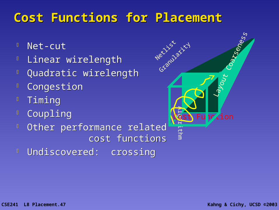
Cost Functions for PlacementCost Functions for PlacementCost Functions for PlacementCost Functions for Placement
Net-cut Linear wirelength Quadratic wirelength Congestion Timing Coupling Other performance related
cost functions Undiscovered: crossing
Net-cut Linear wirelength Quadratic wirelength Congestion Timing Coupling Other performance related
cost functions Undiscovered: crossing
Algorithm
Cost Function
Netlist
Granula
rity
Layo
ut C
oars
enes
s
CSE241 L8 Placement.48 Kahng & Cichy, UCSD ©2003
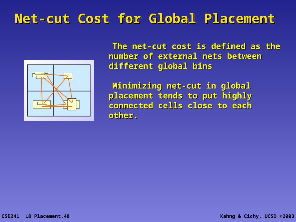
Net-cut Cost for Global PlacementNet-cut Cost for Global PlacementNet-cut Cost for Global PlacementNet-cut Cost for Global Placement
The net-cut cost is defined as the number of The net-cut cost is defined as the number of external nets between different global binsexternal nets between different global bins
Minimizing net-cut in global placement tends Minimizing net-cut in global placement tends to put highly connected cells close to each other.to put highly connected cells close to each other.
CSE241 L8 Placement.49 Kahng & Cichy, UCSD ©2003
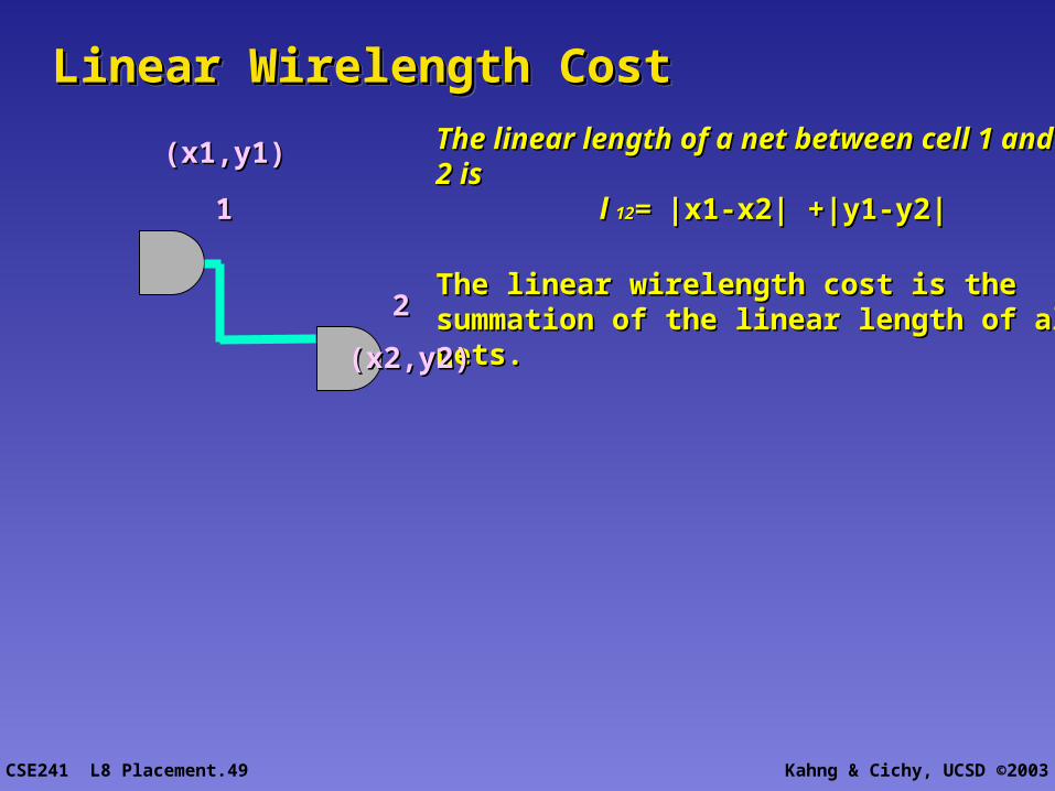
Linear Wirelength Cost Linear Wirelength Cost Linear Wirelength Cost Linear Wirelength Cost
The linear length of a net between cell 1 and cell 2 isThe linear length of a net between cell 1 and cell 2 isll 1212 = = |x1-x2| +|y1-y2||x1-x2| +|y1-y2|
The linear wirelength cost is the summation of the The linear wirelength cost is the summation of the linear length of all nets. linear length of all nets.
(x1,y1)(x1,y1)
(x2,y2)(x2,y2)
11
22
CSE241 L8 Placement.50 Kahng & Cichy, UCSD ©2003
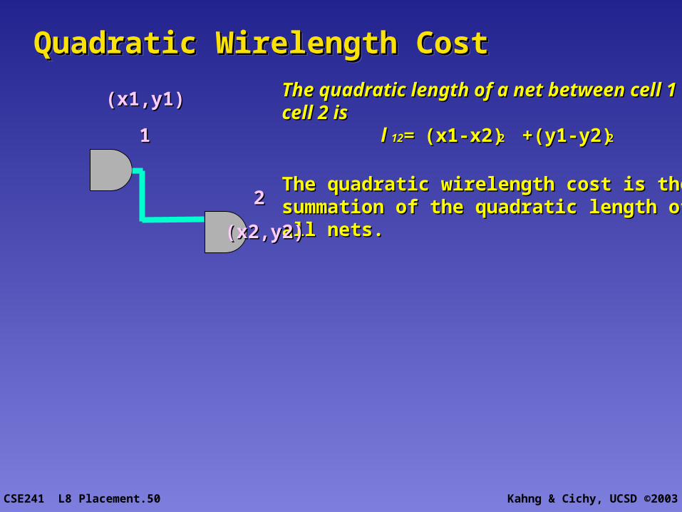
Quadratic Wirelength Cost Quadratic Wirelength Cost Quadratic Wirelength Cost Quadratic Wirelength Cost
The quadratic length of a net between cell 1 and cell 2 The quadratic length of a net between cell 1 and cell 2 isis
ll 1212 = = (x1-x2)(x1-x2)22 +(y1-y2) +(y1-y2)22
The quadratic wirelength cost is the summation of The quadratic wirelength cost is the summation of the quadratic length of all nets. the quadratic length of all nets.
(x1,y1)(x1,y1)
(x2,y2)(x2,y2)
11
22
CSE241 L8 Placement.51 Kahng & Cichy, UCSD ©2003
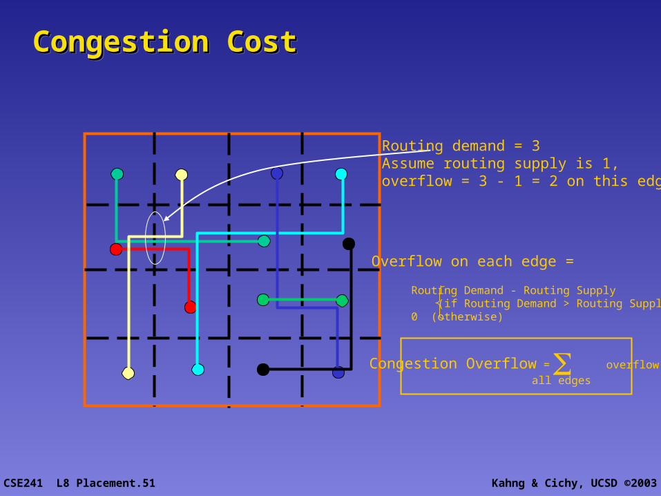
Congestion Cost Congestion Cost Congestion Cost Congestion Cost
Routing demand = 3Assume routing supply is 1,overflow = 3 - 1 = 2 on this edge.
Congestion Overflow = overflowall edges
Overflow on each edge =
Routing Demand - Routing Supply (if Routing Demand > Routing Supply)0 (otherwise)
CSE241 L8 Placement.52 Kahng & Cichy, UCSD ©2003
Cost Functions for PlacementCost Functions for PlacementCost Functions for PlacementCost Functions for Placement
Various cost functions (and a mix of them) have been used in practice to model/estimate routability and timing
We have a good “feel” for what each cost function is capable of doing
We need to understand the interaction among cost functions
Various cost functions (and a mix of them) have been used in practice to model/estimate routability and timing
We have a good “feel” for what each cost function is capable of doing
We need to understand the interaction among cost functions
CSE241 L8 Placement.53 Kahng & Cichy, UCSD ©2003
Congestion Minimization Congestion Minimization and Congestion vs and Congestion vs WirelengthWirelengthCongestion Minimization Congestion Minimization and Congestion vs and Congestion vs WirelengthWirelength
Congestion is important because it closely represents routability (especially at lower-levels of granularity) Congestion is not well understood Ad-hoc techniques have been kind-of working since congestion has never been severe It has been observed that length minimization tends to reduce congestion. Goal: Reduce congestion in placement (willing to sacrifice wirelength a little bit).
Congestion is important because it closely represents routability (especially at lower-levels of granularity) Congestion is not well understood Ad-hoc techniques have been kind-of working since congestion has never been severe It has been observed that length minimization tends to reduce congestion. Goal: Reduce congestion in placement (willing to sacrifice wirelength a little bit).
CSE241 L8 Placement.54 Kahng & Cichy, UCSD ©2003
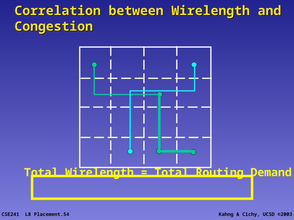
Correlation between Wirelength and Correlation between Wirelength and CongestionCongestionCorrelation between Wirelength and Correlation between Wirelength and CongestionCongestion
Total Wirelength = Total Routing Demand
CSE241 L8 Placement.55 Kahng & Cichy, UCSD ©2003
WirelengthWirelength Congestion CongestionWirelengthWirelength Congestion Congestion
A congestion minimized placement
A wirelength minimized placement
CSE241 L8 Placement.56 Kahng & Cichy, UCSD ©2003
Congestion Map of a Wirelength Minimized Congestion Map of a Wirelength Minimized PlacementPlacementCongestion Map of a Wirelength Minimized Congestion Map of a Wirelength Minimized PlacementPlacement
Congested Spots
CSE241 L8 Placement.57 Kahng & Cichy, UCSD ©2003
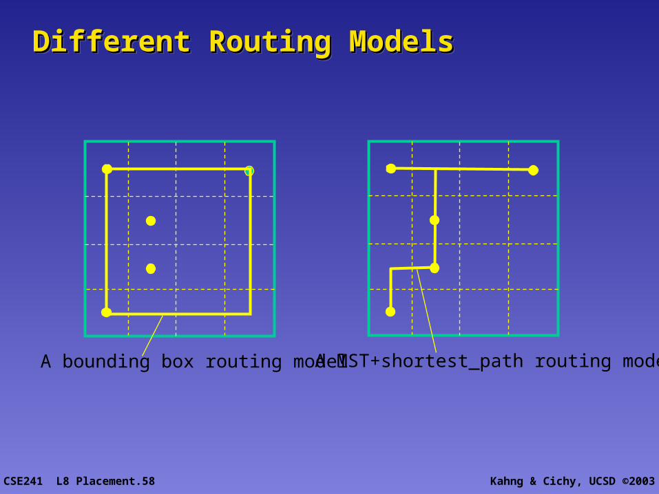
Different Routing Models for modeling Different Routing Models for modeling congestioncongestionDifferent Routing Models for modeling Different Routing Models for modeling congestioncongestion Bounding box router: fast but inaccurate. Real router: accurate but slow. A bounding box router can be used in
placement if it produces correlated routing results with the real router.
Note: For different cost functions, answer might be different (e.g., for coupling, only a detailed router can answer).
Bounding box router: fast but inaccurate. Real router: accurate but slow. A bounding box router can be used in
placement if it produces correlated routing results with the real router.
Note: For different cost functions, answer might be different (e.g., for coupling, only a detailed router can answer).
CSE241 L8 Placement.58 Kahng & Cichy, UCSD ©2003
Different Routing ModelsDifferent Routing ModelsDifferent Routing ModelsDifferent Routing Models
A bounding box routing model A MST+shortest_path routing model
CSE241 L8 Placement.59 Kahng & Cichy, UCSD ©2003
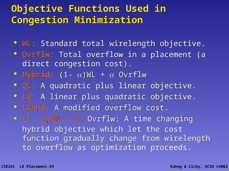
Objective Functions Used in Congestion Objective Functions Used in Congestion MinimizationMinimizationObjective Functions Used in Congestion Objective Functions Used in Congestion MinimizationMinimization
WL: Standard total wirelength objective. Ovrflw: Total overflow in a placement (a direct
congestion cost). Hybrid: (1- )WL + Ovrflw QL: A quadratic plus linear objective. LQ: A linear plus quadratic objective. LkAhd: A modified overflow cost. (1- T)WL + T Ovrflw: A time changing hybrid objective
which let the cost function gradually change from wirelength to overflow as optimization proceeds.
CSE241 L8 Placement.60 Kahng & Cichy, UCSD ©2003
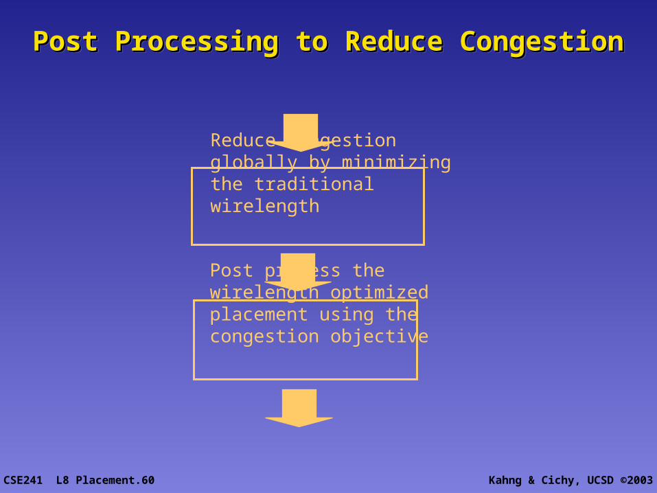
Post Processing to Reduce CongestionPost Processing to Reduce CongestionPost Processing to Reduce CongestionPost Processing to Reduce Congestion
Reduce congestion globally by minimizing the traditional wirelength
Post process the wirelength optimized placement using the congestion objective
CSE241 L8 Placement.61 Kahng & Cichy, UCSD ©2003
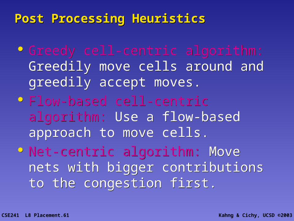
Post Processing HeuristicsPost Processing HeuristicsPost Processing HeuristicsPost Processing Heuristics
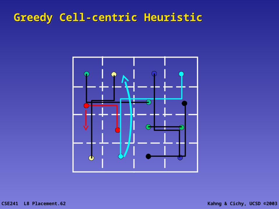
Greedy cell-centric algorithm: Greedily move cells around and greedily accept moves.
Flow-based cell-centric algorithm: Use a flow-based approach to move cells.
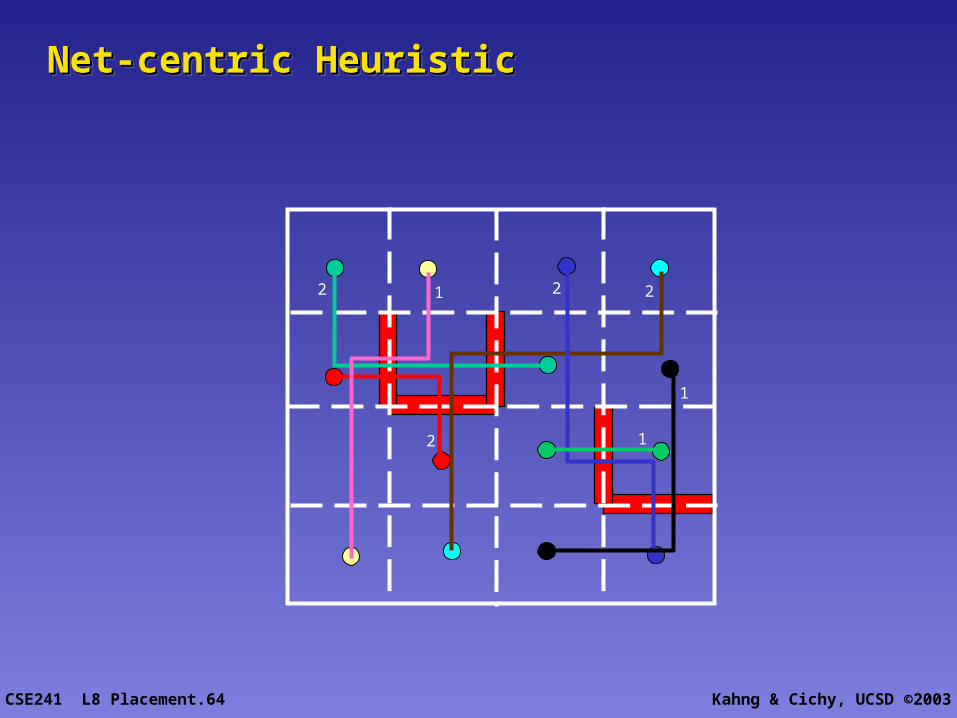
Net-centric algorithm: Move nets with bigger contributions to the congestion first.
Greedy cell-centric algorithm: Greedily move cells around and greedily accept moves.
Flow-based cell-centric algorithm: Use a flow-based approach to move cells.
Net-centric algorithm: Move nets with bigger contributions to the congestion first.
CSE241 L8 Placement.62 Kahng & Cichy, UCSD ©2003
Greedy Cell-centric HeuristicGreedy Cell-centric HeuristicGreedy Cell-centric HeuristicGreedy Cell-centric Heuristic
CSE241 L8 Placement.63 Kahng & Cichy, UCSD ©2003
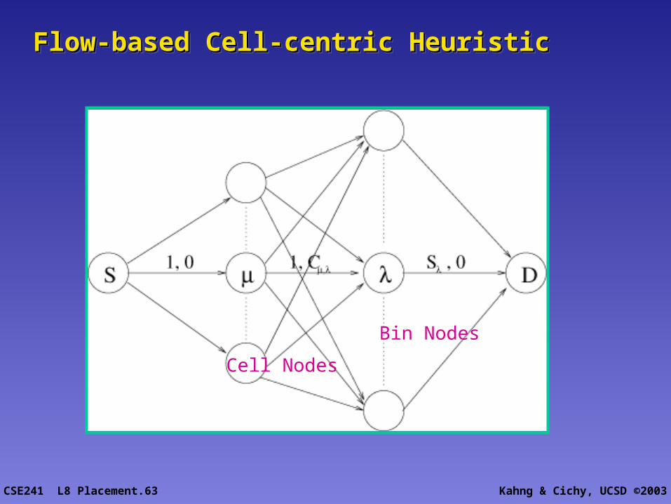
Flow-based Cell-centric HeuristicFlow-based Cell-centric HeuristicFlow-based Cell-centric HeuristicFlow-based Cell-centric Heuristic
Cell Nodes
Bin Nodes
CSE241 L8 Placement.64 Kahng & Cichy, UCSD ©2003
Net-centric HeuristicNet-centric HeuristicNet-centric HeuristicNet-centric Heuristic
2 1
2
2 2
1
1
CSE241 L8 Placement.65 Kahng & Cichy, UCSD ©2003
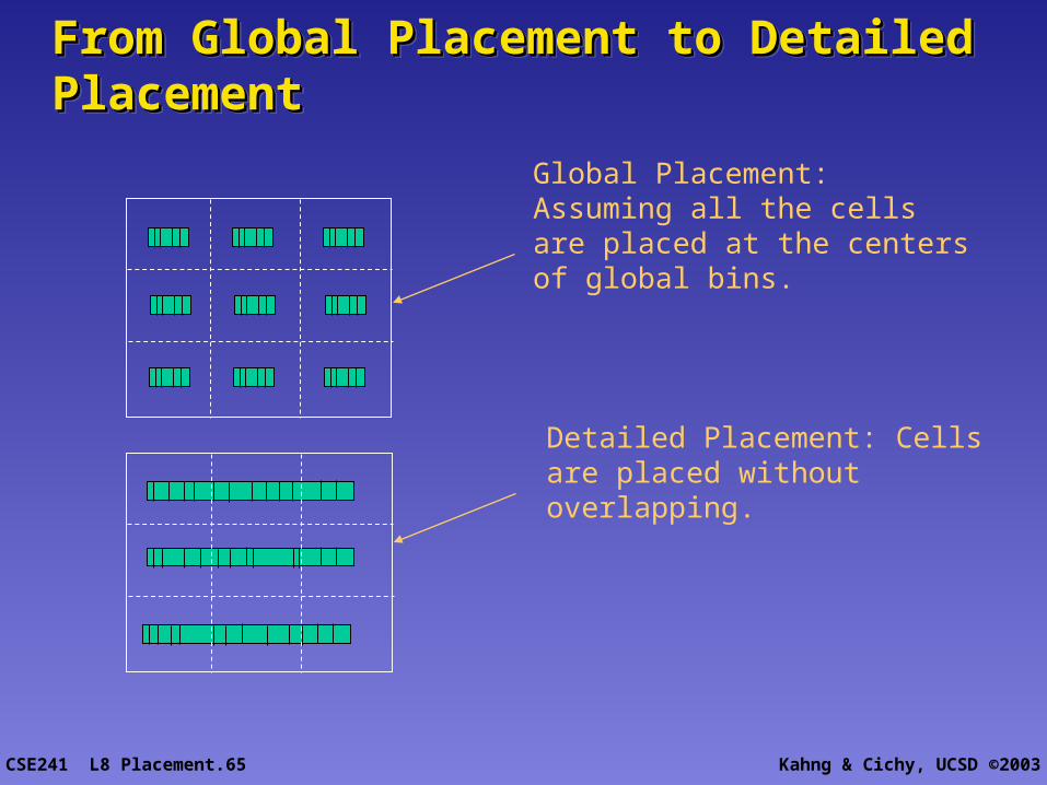
From Global Placement to Detailed From Global Placement to Detailed PlacementPlacementFrom Global Placement to Detailed From Global Placement to Detailed PlacementPlacement
Global Placement: Assuming all the cells are placed at the centers of global bins.
Detailed Placement: Cells are placed without overlapping.
CSE241 L8 Placement.66 Kahng & Cichy, UCSD ©2003
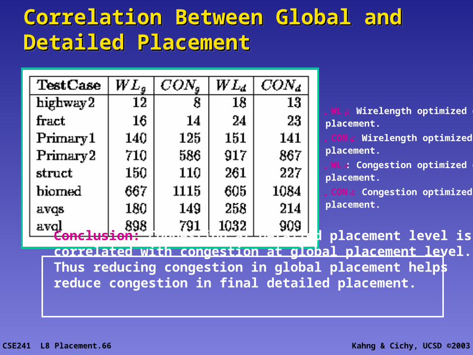
Correlation Between Global and Detailed Correlation Between Global and Detailed PlacementPlacementCorrelation Between Global and Detailed Correlation Between Global and Detailed PlacementPlacement
• WL g: Wirelength optimized global placement.
• CON g: Wirelength optimized detailed placement.
• WL d: Congestion optimized global placement.
• CON d: Congestion optimized detailed placement.
Conclusion: Congestion at detailed placement level is correlated with congestion at global placement level. Thus reducing congestion in global placement helps reduce congestion in final detailed placement.

CSE241 L8 Placement.67 Kahng & Cichy, UCSD ©2003
CongestionCongestionCongestionCongestion
Wirelength minimization can minimize congestion globally. A post processing congestion minimization following wirelength minimization works the best to reduce congestion in placement.
A number of congestion-related cost functions were tested, including a hybrid length plus congestion (commonly believed to be very effective). Experiments prove that they do not work very well.
Net-centric post processing techniques are very effective to minimize congestion.
Congestion at the global placement level, correlates well with congestion of detailed placement.
CSE241 L8 Placement.68 Kahng & Cichy, UCSD ©2003
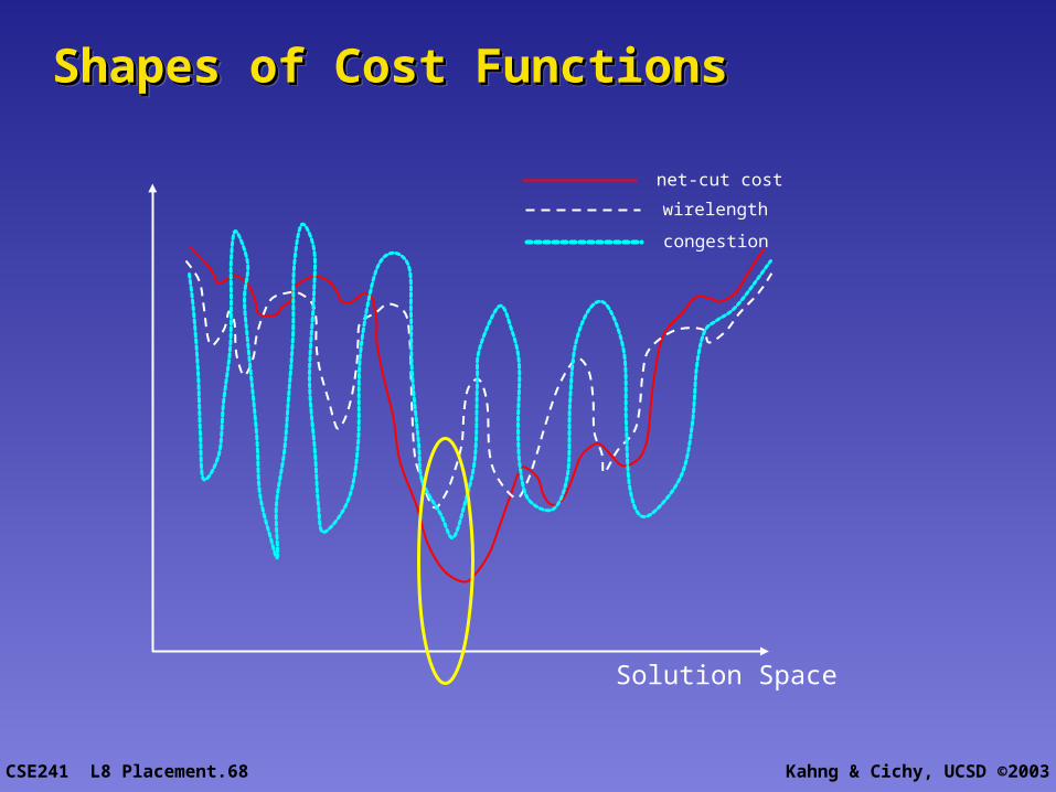
Shapes of Cost FunctionsShapes of Cost FunctionsShapes of Cost FunctionsShapes of Cost Functions
Solution Space
net-cut cost
wirelength
congestion
CSE241 L8 Placement.69 Kahng & Cichy, UCSD ©2003
Relationships Between the Three Cost Relationships Between the Three Cost Functions:Functions:Relationships Between the Three Cost Relationships Between the Three Cost Functions:Functions:
The net-cut objective function is more smooth than the wirelength objective function
The wirelength objective function is more smooth than the congestion objective function
Local minimas of these three objectives are in the same neighborhood.
The net-cut objective function is more smooth than the wirelength objective function
The wirelength objective function is more smooth than the congestion objective function
Local minimas of these three objectives are in the same neighborhood.
CSE241 L8 Placement.70 Kahng & Cichy, UCSD ©2003
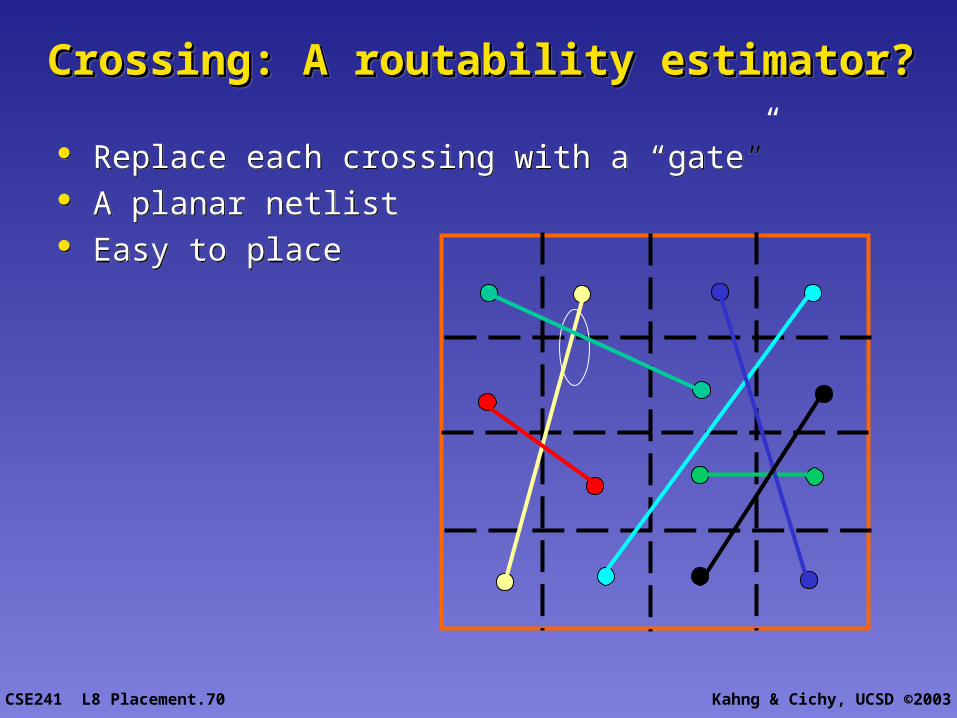
Crossing: A routability estimator?Crossing: A routability estimator?Crossing: A routability estimator?Crossing: A routability estimator?
Replace each crossing with a “gate” A planar netlist Easy to place
Replace each crossing with a “gate” A planar netlist Easy to place
CSE241 L8 Placement.71 Kahng & Cichy, UCSD ©2003
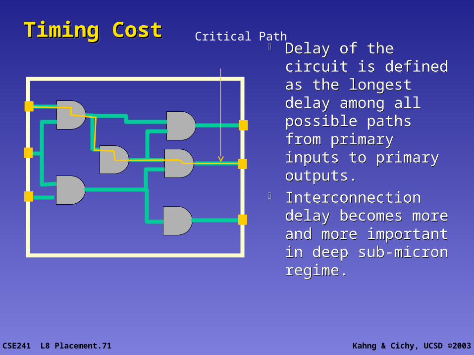
Timing CostTiming CostTiming CostTiming Cost Delay of the circuit is
defined as the longest delay among all possible paths from primary inputs to primary outputs.
Interconnection delay becomes more and more important in deep sub-micron regime.
Delay of the circuit is defined as the longest delay among all possible paths from primary inputs to primary outputs.
Interconnection delay becomes more and more important in deep sub-micron regime.
Critical Path
CSE241 L8 Placement.72 Kahng & Cichy, UCSD ©2003
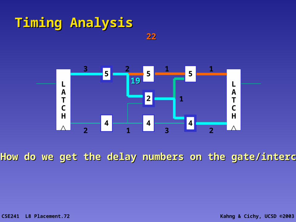
Timing Analysis Timing Analysis
5 5 5
4 4 4
2
LATCH
LATCH
3 2 1 1
2 1 3 2
1
2222
1919
How do we get the delay numbers on the gate/interconnect?How do we get the delay numbers on the gate/interconnect?
CSE241 L8 Placement.73 Kahng & Cichy, UCSD ©2003
ApproachesApproachesApproachesApproaches
Budgeting In accurate information Fast
Path Analysis Most accurate information Very slow
Path analysis with infrequent path substitution Somewhere in between
Budgeting In accurate information Fast
Path Analysis Most accurate information Very slow
Path analysis with infrequent path substitution Somewhere in between
CSE241 L8 Placement.74 Kahng & Cichy, UCSD ©2003
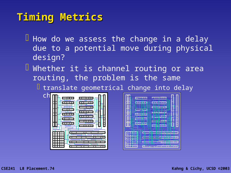
Timing MetricsTiming Metrics
How do we assess the change in a delay due to a potential move during physical design?
Whether it is channel routing or area routing, the problem is the same translate geometrical change into delay change
CSE241 L8 Placement.75 Kahng & Cichy, UCSD ©2003
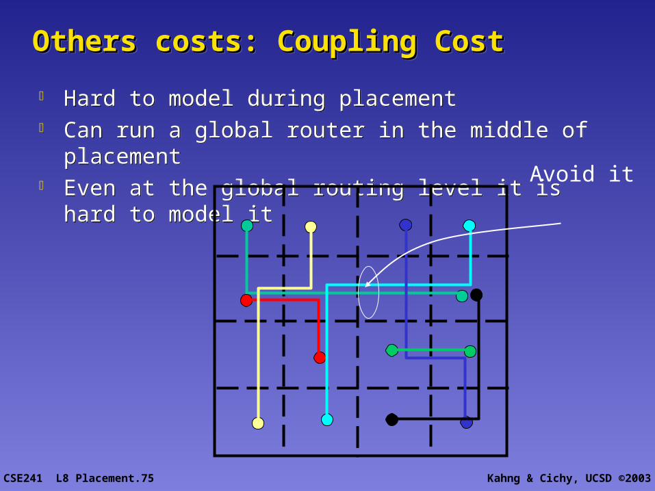
Others costs: Coupling CostOthers costs: Coupling CostOthers costs: Coupling CostOthers costs: Coupling Cost
Hard to model during placement Can run a global router in the middle of placement Even at the global routing level it is hard to model it
Hard to model during placement Can run a global router in the middle of placement Even at the global routing level it is hard to model it
Avoid it
CSE241 L8 Placement.76 Kahng & Cichy, UCSD ©2003
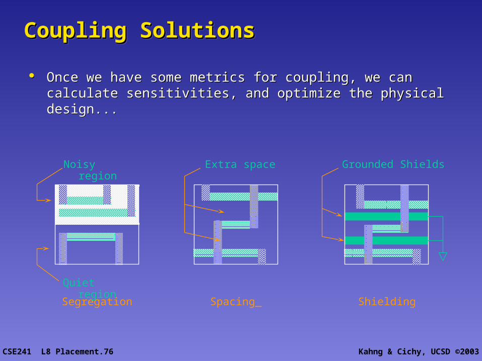
Spacing
Extra space
Segregation
Noisy region
Quiet region
Shielding
Grounded Shields
Coupling SolutionsCoupling SolutionsCoupling SolutionsCoupling Solutions
Once we have some metrics for coupling, we can calculate sensitivities, and optimize the physical design...
Once we have some metrics for coupling, we can calculate sensitivities, and optimize the physical design...
CSE241 L8 Placement.77 Kahng & Cichy, UCSD ©2003
Other Performance CostsOther Performance CostsOther Performance CostsOther Performance Costs
Power usage of the chip. Weighted nets Dual voltages (severe constraint on placement)
Very little known about these cost functions and their interaction with other cost functions
Fundamental research is needed to shed some light on the structure of them
Power usage of the chip. Weighted nets Dual voltages (severe constraint on placement)
Very little known about these cost functions and their interaction with other cost functions
Fundamental research is needed to shed some light on the structure of them
CSE241 L8 Placement.78 Kahng & Cichy, UCSD ©2003
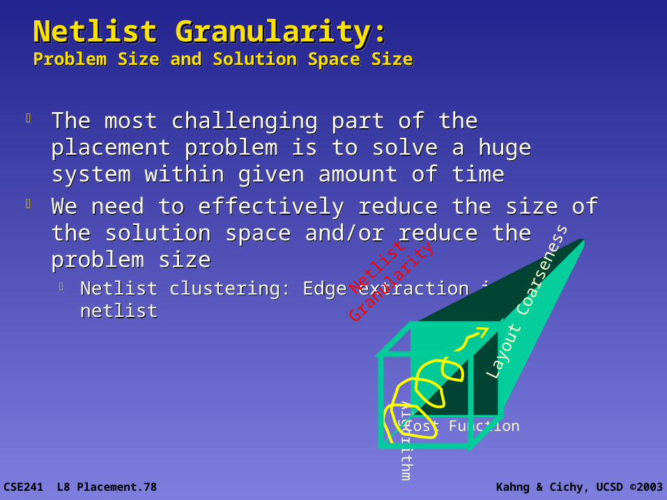
Netlist Granularity: Netlist Granularity: Problem Size and Solution Space SizeProblem Size and Solution Space SizeNetlist Granularity: Netlist Granularity: Problem Size and Solution Space SizeProblem Size and Solution Space Size
The most challenging part of the placement problem is to solve a huge system within given amount of time
We need to effectively reduce the size of the solution space and/or reduce the problem size
Netlist clustering: Edge extraction in the netlist
The most challenging part of the placement problem is to solve a huge system within given amount of time
We need to effectively reduce the size of the solution space and/or reduce the problem size
Netlist clustering: Edge extraction in the netlistA
lgorithm
Cost Function
Netlist
Gran
ularit
y
Layo
ut C
oars
enes
s
CSE241 L8 Placement.79 Kahng & Cichy, UCSD ©2003
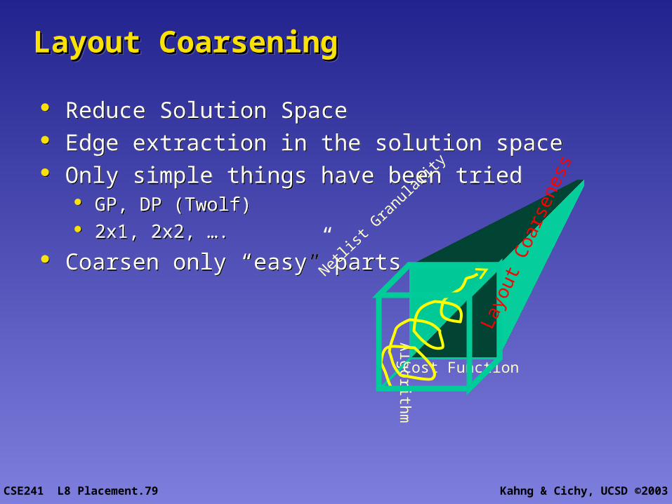
Layout CoarseningLayout CoarseningLayout CoarseningLayout Coarsening
Reduce Solution Space Edge extraction in the solution space Only simple things have been tried
GP, DP (Twolf) 2x1, 2x2, ….
Coarsen only “easy” parts
Reduce Solution Space Edge extraction in the solution space Only simple things have been tried
GP, DP (Twolf) 2x1, 2x2, ….
Coarsen only “easy” partsA
lgorithm
Cost Function
Netlist
Gran
ularit
y
Layo
ut C
oars
enes
s

CSE241 L8 Placement.80 Kahng & Cichy, UCSD ©2003
Incremental PlacementIncremental PlacementIncremental PlacementIncremental Placement
Given an optimal placement for a given netlist, how to construct optimal placements for netlists modified from the given netlist.
Very little research in this area. Different type of incremental changes (in one region, or all over) Methods to use How global should the method be
An extremely important problem.
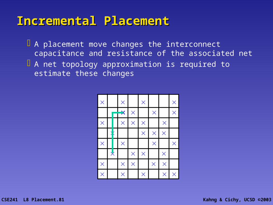
CSE241 L8 Placement.81 Kahng & Cichy, UCSD ©2003
A placement move changes the interconnect capacitance and resistance of the associated net
A net topology approximation is required to estimate these changes
Incremental PlacementIncremental Placement
CSE241 L8 Placement.82 Kahng & Cichy, UCSD ©2003
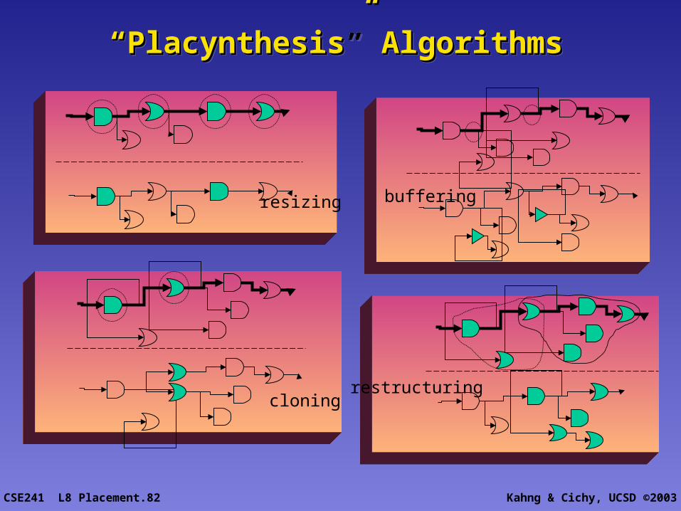
““Placynthesis” Algorithms Placynthesis” Algorithms ““Placynthesis” Algorithms Placynthesis” Algorithms
resizing buffering
cloningrestructuring
CSE241 L8 Placement.83 Kahng & Cichy, UCSD ©2003
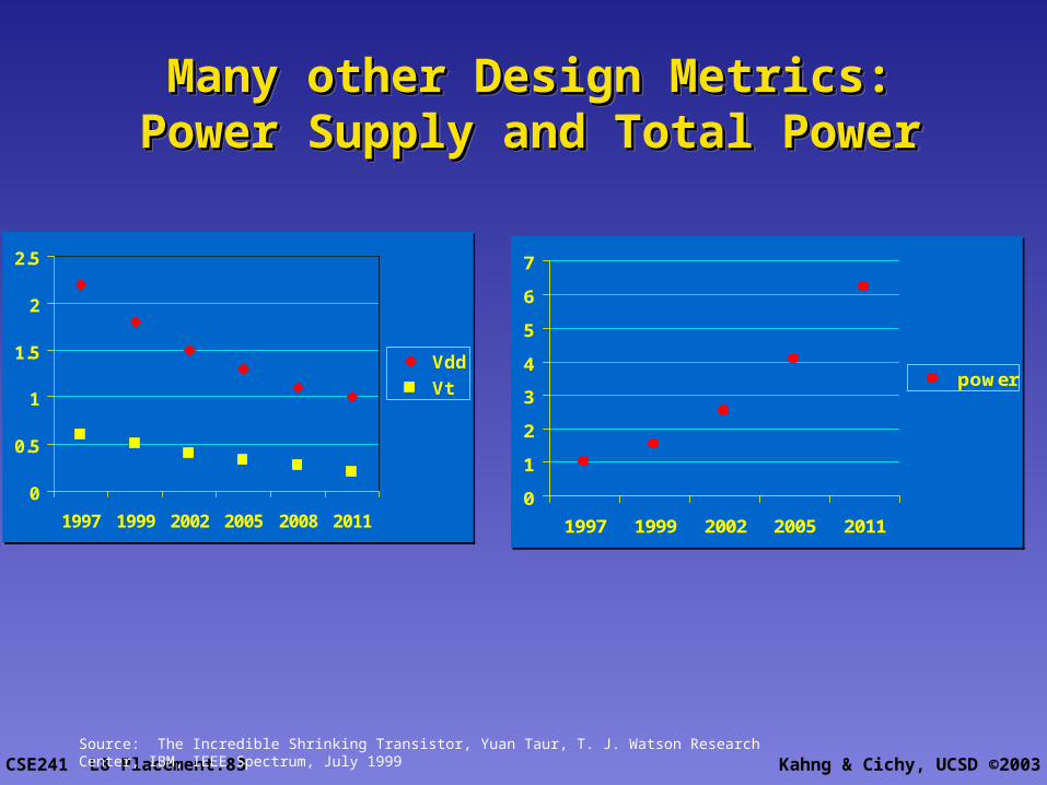
Many other Design Metrics:Many other Design Metrics:Power Supply and Total PowerPower Supply and Total Power
Many other Design Metrics:Many other Design Metrics:Power Supply and Total PowerPower Supply and Total Power
0
0.5
1
1.5
2
2.5
1997 1999 2002 2005 2008 2011
Vdd
Vt
Source: The Incredible Shrinking Transistor, Yuan Taur, T. J. Watson Research Center, IBM, IEEE Spectrum, July 1999
0
1
2
3
4
5
6
7
1997 1999 2002 2005 2011
power
CSE241 L8 Placement.84 Kahng & Cichy, UCSD ©2003
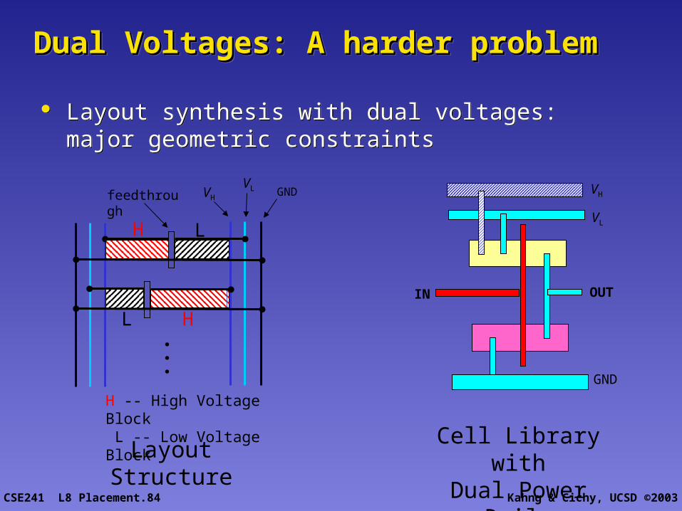
HL
H L
feedthrough VH
VL GND
H -- High Voltage Block L -- Low Voltage Block
Layout Structure
VH
VL
Cell Library withDual Power Rails
GND
IN OUT
Dual Voltages: A harder problemDual Voltages: A harder problemDual Voltages: A harder problemDual Voltages: A harder problem
Layout synthesis with dual voltages: major geometric constraints
Layout synthesis with dual voltages: major geometric constraints


