50
CSIS 7102 Spring 2004 Lecture 5 : Non-locking based concurrency control (and some more lock-based ones, too) Dr. King-Ip Lin
| Date post: | 14-Dec-2015 |
| Category: |
Documents |
| Upload: | dianna-anguish |
| View: | 219 times |
| Download: | 0 times |

CSIS 7102 Spring 2004Lecture 5 : Non-locking based concurrency control (and some more lock-based ones, too)
Dr. King-Ip Lin
Table of contents
Limitation of locking techniques Timestamp ordering View serializability Optimistic concurrency control Graph-based locking Multi-version schemes

The story so far
Two-phase locking (2PL) as a protocol to ensure conflict serializability Once a transaction start releasing locks, cannot
obtain new locks Ensure that the conflict cannot go both direction
Deadlock handling in 2PL The phantom problem Multi-granularity locking
Intention locks Improving concurrency while maintaining correctness
Levels of isolation Not every transaction need 2PL to be correct Ability to define which isolation level for a transaction
to be run Enable even higher concurrency

Limitation of lock-based techniques
Lock-based techniques ensure correctness
However, it tends to be a bit “pessimistic” Some schedules that are serializable
will not be allowed under the locking protocol.
Limitation of lock-based techniques
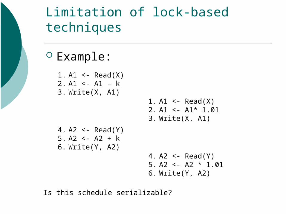
Example:
1. A1 <- Read(X)2. A1 <- A1 – k3. Write(X, A1)
4. A2 <- Read(Y)5. A2 <- A2 + k6. Write(Y, A2)
1. A1 <- Read(X)2. A1 <- A1* 1.013. Write(X, A1)
4. A2 <- Read(Y)5. A2 <- A2 * 1.016. Write(Y, A2)
Is this schedule serializable?

Limitation of lock-based techniques
However, 2PL does not allow it
1. A1 <- Read(X)2. A1 <- A1 – k3. Write(X, A1)
4. A2 <- Read(Y)5. A2 <- A2 + k6. Write(Y, A2)
1. A1 <- Read(X)2. A1 <- A1* 1.013. Write(X, A1)
4. A2 <- Read(Y)5. A2 <- A2 * 1.016. Write(Y, A2)
Blocked (T1 already has X-lock); T2 cannot proceed

Limitation of lock-based techniques
Why does 2PL block this operation? There is a conflict between T1 and T2 If we allow T2 to go on, there is a
potential danger that T2 can finish before T1 resumes, which leads to a non-serializable schedule
Thus, 2PL decide to “play safe”

Limitation of lock-based techniques
But is 2PL “playing TOO safe”?
1. A1 <- Read(X)2. A1 <- A1 – k3. Write(X, A1)
4. A2 <- Read(Y)5. A2 <- A2 + k6. Write(Y, A2)
1. A1 <- Read(X)2. A1 <- A1* 1.013. Write(X, A1)4. A2 <- Read(Y)5. A2 <- A2 * 1.016. Write(Y, A2)
Schedule may still be serializable if we allow this
Only if we allow this to go before T1 resume, then the schedule becomes unserializable

Limitation of lock-based techniques
In some cases, 2PL is playing too safe Can we allow for more concurrency? (e.g. allow
some conflicting operation to go ahead, until we can determine that a schedule is not serializable)
One method: dynamically keep track of serializability graph Check before each operation to see if a cycle will
appear Not practical
A more practical approach: predefine allowable conflict operations, so that a cycle is never formed Timestamps
Timestamp ordering
Timestamp (TS): a number associated with each transaction Not necessarily real time
Can be assigned by a logical counter Unique for each transaction Should be assigned in an increasing
order for each new transaction
Timestamp ordering
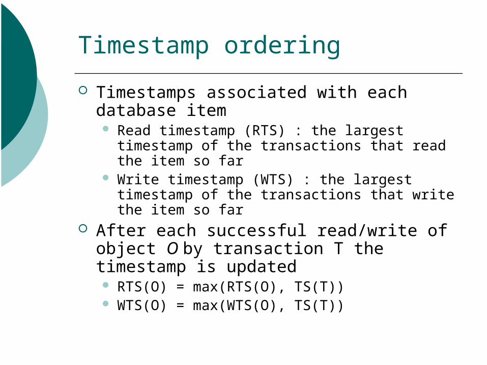
Timestamps associated with each database item Read timestamp (RTS) : the largest timestamp
of the transactions that read the item so far Write timestamp (WTS) : the largest timestamp
of the transactions that write the item so far After each successful read/write of object
O by transaction T the timestamp is updated RTS(O) = max(RTS(O), TS(T)) WTS(O) = max(WTS(O), TS(T))
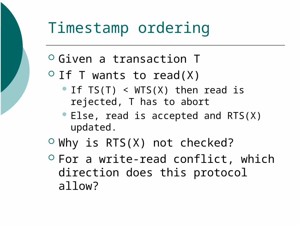
Timestamp ordering
Given a transaction T If T wants to read(X)
If TS(T) < WTS(X) then read is rejected, T has to abort
Else, read is accepted and RTS(X) updated.
Why is RTS(X) not checked? For a write-read conflict, which
direction does this protocol allow?
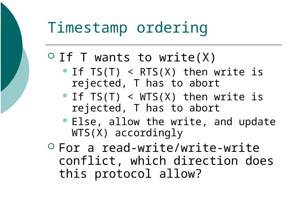
Timestamp ordering
If T wants to write(X) If TS(T) < RTS(X) then write is rejected,
T has to abort If TS(T) < WTS(X) then write is rejected,
T has to abort Else, allow the write, and update
WTS(X) accordingly For a read-write/write-write conflict,
which direction does this protocol allow?

Timestamp ordering -- example
Consider the two transactions
1. A1 <- Read(X)2. A1 <- A1* 1.013. Write(X, A1)4. A2 <- Read(Y)5. A2 <- A2 * 1.016. Write(Y, A2)
1. A1 <- Read(X)2. A1 <- A1 – k3. Write(X, A1)4. A2 <- Read(Y)5. A2 <- A2 + k6. Write(Y, A2)
T1 (TS = 10) T2 (TS = 20)
Initially all RTS and WTS = 0

Timestamp ordering -- example
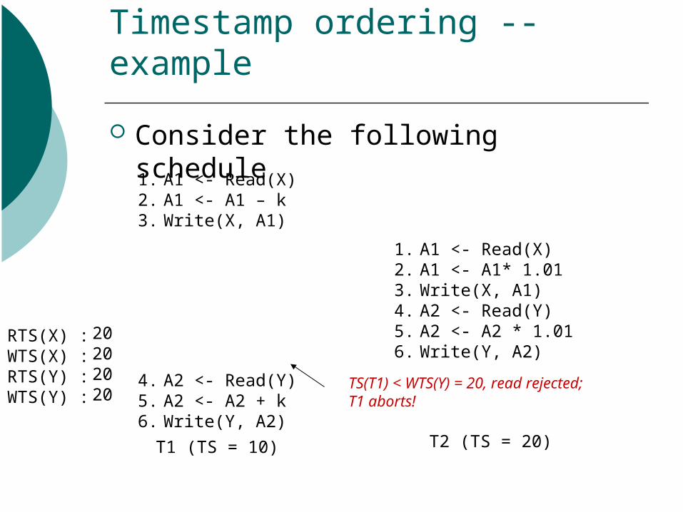
Consider the following schedule
1. A1 <- Read(X)2. A1 <- A1* 1.013. Write(X, A1)
4. A2 <- Read(Y)5. A2 <- A2 * 1.016. Write(Y, A2)
1. A1 <- Read(X)2. A1 <- A1 – k3. Write(X, A1)
4. A2 <- Read(Y)5. A2 <- A2 + k6. Write(Y, A2)
T1 (TS = 10) T2 (TS = 20)
TS(T1) > WTS(X) = 0, read allowed;RTS(X) 10
RTS(X) : WTS(X) : RTS(Y) : WTS(Y) :
0000
10000
TS(T1) > WTS(X) = 0;TS(T1) = RTS(X) = 10; write allowed;WTS(X) 10
101000

Timestamp ordering -- example
Consider the following schedule
1. A1 <- Read(X)2. A1 <- A1* 1.013. Write(X, A1)
4. A2 <- Read(Y)5. A2 <- A2 * 1.016. Write(Y, A2)
1. A1 <- Read(X)2. A1 <- A1 – k3. Write(X, A1)
4. A2 <- Read(Y)5. A2 <- A2 + k6. Write(Y, A2)
T1 (TS = 10) T2 (TS = 20)
TS(T2) > WTS(X) = 10, read allowed;RTS(X) 20
RTS(X) : WTS(X) : RTS(Y) : WTS(Y) :
201000
TS(T2) = RTS(X) = 20TS(T2) > WTS(X) = 10, write allowed;WTS(X) 20
202000

Timestamp ordering -- example
Consider the following schedule
1. A1 <- Read(X)2. A1 <- A1* 1.013. Write(X, A1)
4. A2 <- Read(Y)5. A2 <- A2 * 1.016. Write(Y, A2)
1. A1 <- Read(X)2. A1 <- A1 – k3. Write(X, A1)
4. A2 <- Read(Y)5. A2 <- A2 + k6. Write(Y, A2)
T1 (TS = 10) T2 (TS = 20)
RTS(X) : WTS(X) : RTS(Y) : WTS(Y) :
20201010
Similarly, at the end of this step

Timestamp ordering -- example
Consider the following schedule
1. A1 <- Read(X)2. A1 <- A1* 1.013. Write(X, A1)
4. A2 <- Read(Y)5. A2 <- A2 * 1.016. Write(Y, A2)
1. A1 <- Read(X)2. A1 <- A1 – k3. Write(X, A1)
4. A2 <- Read(Y)5. A2 <- A2 + k6. Write(Y, A2)
T1 (TS = 10) T2 (TS = 20)
TS(T2) > WTS(Y) = 10, read allowed;RTS(Y) 20
RTS(X) : WTS(X) : RTS(Y) : WTS(Y) :
20202010
TS(T2) = RTS(Y) = 20TS(T2) > WTS(Y) = 10, write allowed;WTS(Y) 20
20202020
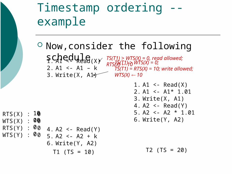
Timestamp ordering -- example
Now,consider the following schedule
1. A1 <- Read(X)2. A1 <- A1* 1.013. Write(X, A1)4. A2 <- Read(Y)5. A2 <- A2 * 1.016. Write(Y, A2)
1. A1 <- Read(X)2. A1 <- A1 – k3. Write(X, A1)
4. A2 <- Read(Y)5. A2 <- A2 + k6. Write(Y, A2)
T1 (TS = 10) T2 (TS = 20)
TS(T1) > WTS(X) = 0, read allowed;RTS(X) 10
RTS(X) : WTS(X) : RTS(Y) : WTS(Y) :
0000
10000
TS(T1) > WTS(X) = 0;TS(T1) = RTS(X) = 10; write allowed;WTS(X) 10
101000

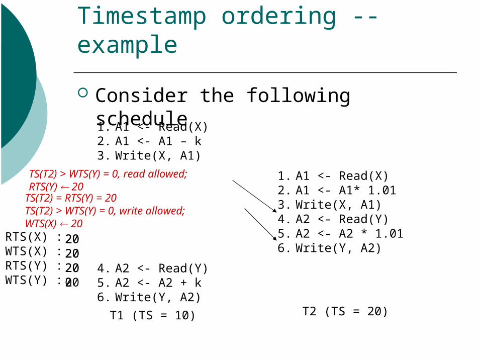
Timestamp ordering -- example
Consider the following schedule
1. A1 <- Read(X)2. A1 <- A1* 1.013. Write(X, A1)4. A2 <- Read(Y)5. A2 <- A2 * 1.016. Write(Y, A2)
1. A1 <- Read(X)2. A1 <- A1 – k3. Write(X, A1)
4. A2 <- Read(Y)5. A2 <- A2 + k6. Write(Y, A2)
T1 (TS = 10) T2 (TS = 20)
TS(T2) > WTS(X) = 10, read allowed;RTS(X) 20
RTS(X) : WTS(X) : RTS(Y) : WTS(Y) :
201000
TS(T2) = RTS(X) = 20TS(T2) > WTS(X) = 10, write allowed;WTS(X) 20
202000
Timestamp ordering -- example
Consider the following schedule
1. A1 <- Read(X)2. A1 <- A1* 1.013. Write(X, A1)4. A2 <- Read(Y)5. A2 <- A2 * 1.016. Write(Y, A2)
1. A1 <- Read(X)2. A1 <- A1 – k3. Write(X, A1)
4. A2 <- Read(Y)5. A2 <- A2 + k6. Write(Y, A2)
T1 (TS = 10) T2 (TS = 20)
TS(T2) > WTS(Y) = 0, read allowed;RTS(Y) 20
RTS(X) : WTS(X) : RTS(Y) : WTS(Y) :
2020200
TS(T2) = RTS(Y) = 20TS(T2) > WTS(Y) = 0, write allowed;WTS(X) 20
20202020
Timestamp ordering -- example
Consider the following schedule
1. A1 <- Read(X)2. A1 <- A1* 1.013. Write(X, A1)4. A2 <- Read(Y)5. A2 <- A2 * 1.016. Write(Y, A2)
1. A1 <- Read(X)2. A1 <- A1 – k3. Write(X, A1)
4. A2 <- Read(Y)5. A2 <- A2 + k6. Write(Y, A2)
T1 (TS = 10) T2 (TS = 20)
TS(T1) < WTS(Y) = 20, read rejected;T1 aborts!
RTS(X) : WTS(X) : RTS(Y) : WTS(Y) :
20202020
Timestamp ordering
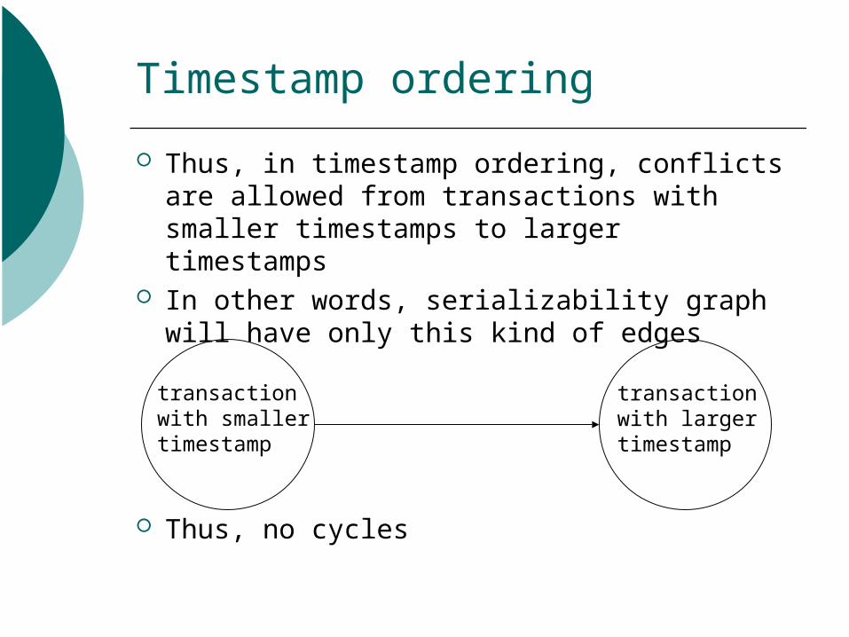
Thus, in timestamp ordering, conflicts are allowed from transactions with smaller timestamps to larger timestamps
In other words, serializability graph will have only this kind of edges
Thus, no cycles
transactionwith smallertimestamp
transactionwith largertimestamp
Timestamp ordering – good & bad
Advantages of timestamp ordering No waiting for transaction Thus, no deadlocks
Disadvantages Schedule may not be recoverable (see
previous example) Why?
Long transaction may be aborted more often
Why?

Timestamp ordering – overcoming disadvantages
Solution for recoverability Forcing all writes at the end of transactions; as
well as making writes atomic (no other transaction can access any written item until all are written)
Block (only) reading of dirty items (using locks) Use idea of commit dependency (discussed
later) Solution for starvation
Assign new timestamp for aborted transaction Temporary block short transactions to allow
long transaction to go on (tricky to implement)
Locks -- implementation
Various support need to implement locking OS support – lock(X) must be an atomic
operation in the OS level i.e. support for critical sections
Implementation of read(X)/write(X) – automatically add code for locking
Lock manager – module to handle and keep track of locks
Thomas’ write rule
Write-write conflict may be acceptable in many cases
Suppose T1 do a write(X) and then T2 do a write(X) and there is no transaction accessing X in between
Then T2 only overwrite a value that is never being used
In such case, it can be argued that such a write is acceptable

Thomas’ write rule
In timestamp ordering, it is referred as the Thomas write rule:
If a transaction T issue a write(X): If TS(T) < RTS(X) then write is rejected, T has
to abort Else If TS(T) < WTS(X) then write is ignored Else, allow the write, and update WTS(X)
accordingly A schedule allowed by Thomas write rule
may not be conflict serializable, but is known to be view serializable.

View serializability
Let S and S´ be two schedules with the same set of transactions. S and S´ are view equivalent if the following three conditions are met:1. For each data item Q, if transaction Ti reads the
initial value of Q in schedule S, then transaction Ti must, in schedule S´, also read the initial value of Q.
2. For each data item Q if transaction Ti executes read(Q) in schedule S, and that value was produced by transaction Tj (if any), then transaction Ti must in schedule S´ also read the value of Q that was produced by transaction Tj .
3. For each data item Q, the transaction (if any) that performs the final write(Q) operation in schedule S must perform the final write(Q) operation in schedule S´.

View serializability
View equivalence is also based purely on reads and writes alone.
Roughly speaking, for two view equivalent schedules, each corresponding read(X) read the
same value (including initial read) Strictly speaking, it is stronger, as it is
required to be the value produced by the same transaction
The final value of each X has to be written by the same corresponding transaction(s)

View serializability
A schedule is view serializable if it is view equivalent to a serial schedule
Conflict serializable view serializable But NOT vice versa
This schedule is view serializable to the schedule (T1, T2, T3) but not conflict serializable (R-W conflict T1->T2, W-W conflict T2->T1)
1. Read(X)
2. Write(X)1. Write(X)
1. Write(X)
T1 T2 T3

View serializability
Blind writes: writes that write values not based on previous reads
View serializability = conflict serializability + blind writes
Currently, view serializability is not very practical Determining whether a schedule is view
serializable is NP-complete
1. Read(X)
2. Write(X)1. Write(X)
1. Write(X)
T1 T2 T3
Blind writes

Optimistic concurrency control
Timestamp ordering is more optimistic then 2PL It does not block operation Enable conflict in one direction to proceed
immediately It still has limitation
Need care to handle recoverability Overhead in maintain timestamps (and space)
It is still a waste of time if we have very few conflicts
Can we be even more optimistic

Optimistic concurrency control
Most optimistic point-of-view: Assume no problem and let transaction
execute But before commit, do a final check Only when a problem is discovered,
then one aborts Basis for optimistic concurrency
control

Optimistic concurrency control
Each transaction T is divided into 3 phases:
1. Read and execution: T reads from the database and execute. However, T only writes to temporary location (not to the database iteself)
2. Validation: T checks whether there is conflict with other transaction, abort if necessary
3. Write : T actually write the values in temporary location to the database
Each transaction must follow the same order

Optimistic concurrency control
Each transaction T is given 3 timestamps:
Start(T): when the transaction starts Validation(T): when the transaction
enters the validation phase Finish(T) : when the transaction
finishes Goal: to ensure the transaction
following a serial schedule based on Validation(T)

Optimistic concurrency control
Given two transaction T1 and T2
and Validation(T1) < Validation(T2)
Case 1 : Finish(T1) < Start(T2)
Time
Read Valid WriteT1 :
Start(T1) Valid(T1) Finish(T1)
Read Valid WriteT2 :
Start(T2) Valid(T2) Finish(T2)
Here, no problem of serializability

Optimistic concurrency control
Case 2 : Finish(T1) < Validation(T2)
Time
Read Valid WriteT1 :
Start(T1) Valid(T1) Finish(T1)
T2 :Read Valid Write
Start(T2) Valid(T2) Finish(T2)
If T2 does not read anything T1 writes, then no problem
Potential conflict

Optimistic concurrency control
Case 3 : Validation(T2) < Finish(T1)
Time
Read Valid WriteT1 :
Start(T1) Valid(T1) Finish(T1)
T2 :Read Valid Write
Start(T2) Valid(T2) Finish(T2)
If T2 does not read or writes anything T1 writes, then no problem
Potential conflict
Optimistic concurrency control
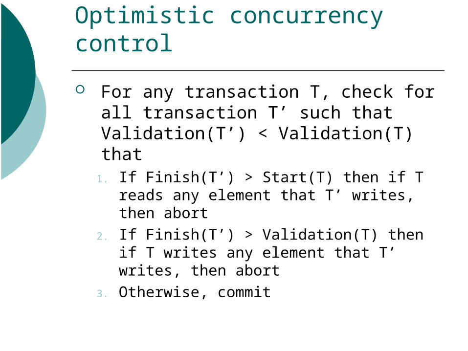
For any transaction T, check for all transaction T’ such that Validation(T’) < Validation(T) that
1. If Finish(T’) > Start(T) then if T reads any element that T’ writes, then abort
2. If Finish(T’) > Validation(T) then if T writes any element that T’ writes, then abort
3. Otherwise, commit
Optimistic concurrency control
Advantages: No blocking No overhead during execution
Do have overhead for validation No cascade rollbacks (why?)
Disadvantages: Potential starvation for long
transaction Large amount of aborts if high
concurrency

Graph-based locking
2 phased locking make no assumption about behavior of transactions
If we have some assumptions/knowledge about how data is accessed, we can make use of it to find more efficient/optimistic locking techniques

Graph-based locking
Suppose we make the following assumptions There is an partial ordering of the
database items such that if X < Y, then a transaction must access X before it access Y (regardless whether the transaction uses X or not)
The graph formed by the partial order is a tree
Only X-locks are allowed
Graph-based locking
A transaction T must follow the following rules The first lock by T can be of any item After that, an item X can be locked only
when T has a lock on the parent of X Unlock can be done at anytime, but... … once an item is unlocked, it cannot
be relocked

Graph-based locking
Example of valid actions: Lock(B), Lock(E),
Lock(D), Unlock(B), Unlock(E), Lock(G),Unlock(D), Unlock(G)
Lock(D), Lock(H), Unlock(D), Unlock(H)

Graph-based locking
Advantages No deadlocks No need to be 2-phase
Earlier release on locks, thus higher concurrency
Disadvantages One may have to lock things that it
does not need Example, from last slide, if T needs D and
J, then it must lock H also. Schedule may be unrecoverable

Graph-based locking
Solution for non-recoverability Hold X-locks until end of transaction
But reduce concurrency significantly If one can tolerate cascade aborts, then use
notion of commit dependency For every item that is written (but not yet
committed) record the transaction T that perform the write
If a transaction T’ read such data, then we declare T’ has a commit dependency on T
T’ cannot commit until T commits T’ must abort if T aborts.

Multi-version schemes
Consider a write-read conflict in a 2PL scheme
T1 obtained a X-lock on an item, and T2 has to wait
Why T2 wait? Potential conflict that goes both ways Unsure of whether the value written by T1 is
trustworthy (as T1 has not committed yet) What if we kept the old values of the item
so that T2 can choose the appropriate version of the values to read?
multi-version concurrency control

Multi-version timestamp ordering
Each data item Q has a sequence of versions <Q1, Q2,...., Qm>. Each version Qk contains three data fields: Content -- the value of version Qk. W-timestamp(Qk) -- timestamp of the transaction that
created (wrote) version Qk
R-timestamp(Qk) -- largest timestamp of a transaction that successfully read version Qk
when a transaction Ti creates a new version Qk of Q, Qk's W-timestamp and R-timestamp are initialized to TS(Ti).
R-timestamp of Qk is updated whenever a transaction Tj reads Qk, and TS(Tj) > R-timestamp(Qk).

Multi-version timestamp ordering
Suppose that transaction Ti issues a read(Q) or write(Q)
operation. Let Qk denote the version of Q whose write
timestamp is the largest write timestamp less than or equal to TS(Ti).
1. If transaction Ti issues a read(Q), then the value returned is the content of version Qk.
2. If transaction Ti issues a write(Q), and if TS(Ti) < R- timestamp(Qk), then transaction Ti is rolled back. Otherwise, if TS(Ti) = W-timestamp(Qk), the contents of Qk are overwritten, otherwise a new version of Q is created. Reads always succeed; a write by Ti is rejected if some other
transaction Tj that (in the serialization order defined by the timestamp values) should read Ti's write, has already read a version created by a transaction older than Ti.


