Page 1
V1 Spring 2017・CTL.SC0x – Supply Chain Analytics Key Concepts・MITx MicroMasters in Supply Chain Management MIT Center for Transportation & Logistics・Cambridge, MA 02142 USA ・[email protected] This work is licensed under a Creative Commons Attribution-NonCommercial-ShareAlike 4.0 International License. 1
CTL.SC0x-SupplyChainAnalytics
KeyConceptsDocumentThisdocumentcontainstheKeyConceptsfortheSC0xcourse.Thedocumentisbasedonapastrunofthecourseanddoesnotincludeallthematerialthatwillbeincludedinthiscourse;pleasecheckbackfornewerversionsofthedocumentthroughoutthecourse.Thesearemeanttocomplement,notreplace,thelessonvideosandslides.Theyareintendedtobereferencesforyoutousegoingforwardandarebasedontheassumptionthatyouhavelearnedtheconceptsandcompletedthepracticeproblems.ThedraftwascreatedbyDr.AlexisBatemanintheSpringof2017.Thisisadraftofthematerial,sopleasepostanysuggestions,corrections,orrecommendationstotheDiscussionForumunderthetopicthread“KeyConceptDocumentsImprovements.”Thanks,ChrisCaplice,EvaPonceandtheSC0xTeachingCommunitySpring2017v1
Page 2
V1 Spring 2017・CTL.SC0x – Supply Chain Analytics Key Concepts・MITx MicroMasters in Supply Chain Management MIT Center for Transportation & Logistics・Cambridge, MA 02142 USA ・[email protected] This work is licensed under a Creative Commons Attribution-NonCommercial-ShareAlike 4.0 International License. 2
TableofContentsSupplyChainIntro................................................................................................................................3
Models,Algebra,&Functions...............................................................................................................6Models.....................................................................................................................................................6Functions..................................................................................................................................................6QuadraticFunctions.................................................................................................................................7ConvexityandContinuity.........................................................................................................................8
Optimization........................................................................................................................................9UnconstrainedOptimization....................................................................................................................9ConstrainedOptimization......................................................................................................................11LinearPrograms.....................................................................................................................................11IntegerandMixedIntegerPrograms.....................................................................................................14
AdvancedOptimization......................................................................................................................18NetworkModels.....................................................................................................................................18Non-LinearOptimization........................................................................................................................20
AlgorithmsandApproximations.........................................................................................................23Algorithms..............................................................................................................................................23ShortestPathProblem...........................................................................................................................24VehicleRoutingProblem........................................................................................................................25ApproximationMethods........................................................................................................................29
DistributionsandProbability..............................................................................................................36Probability..............................................................................................................................................36Summarystatistics.................................................................................................................................37ProbabilityDistributions.........................................................................................................................40
Regression..........................................................................................................................................47MultipleRandomVariables....................................................................................................................47InferenceTesting....................................................................................................................................49OrdinaryLeastSquaresLinearRegression.............................................................................................54
Simulation..........................................................................................................................................58Simulation..............................................................................................................................................58StepsinaSimulationStudy....................................................................................................................58
References.........................................................................................................................................61
Page 3
V1 Spring 2017・CTL.SC0x – Supply Chain Analytics Key Concepts・MITx MicroMasters in Supply Chain Management MIT Center for Transportation & Logistics・Cambridge, MA 02142 USA ・[email protected] This work is licensed under a Creative Commons Attribution-NonCommercial-ShareAlike 4.0 International License. 3
SupplyChainIntro
SummarySupplyChainBasicsisanoverviewoftheconceptsofSupplyChainManagementandlogistics.Itdemonstratesthatproductsupplychainsasvariedasbananastowomen’sshoestocementhavecommonsupplychainelements.Therearemanydefinitionsofsupplychainmanagement.Butultimatelysupplychainsarethephysical,financial,andinformationflowbetweentradingpartnersthatultimatelyfulfillacustomerrequest.Theprimarypurposeofanysupplychainistosatisfyacustomer’sneedattheendofthesupplychain.Essentiallysupplychainsseektomaximizethetotalvaluegeneratedasdefinedas:theamountthecustomerpaysminusthecostoffulfillingtheneedalongtheentiresupplychain.Allsupplychainsincludemultiplefirms.
KeyConceptsWhileSupplyChainManagementisanewterm(firstcoinedin1982byKeithOliverfromBoozAllenHamiltoninaninterviewwiththeFinancialTimes),theconceptsareancientanddatebacktoancientRome.Theterm“logistics”hasitsrootsintheRomanmilitary.Additionaldefinitions:
• Logisticsinvolves…“managingtheflowofinformation,cashandideasthroughthecoordinationofsupplychainprocessesandthroughthestrategicadditionofplace,periodandpatternvalues”–MITCenterforTransportationandLogistics
• “SupplyChainManagementdealswiththemanagementofmaterials,informationandfinancialflowsinanetworkconsistingofsuppliers,manufacturers,distributors,andcustomers”-StanfordSupplyChainForum
• “Callitdistributionorlogisticsorsupplychainmanagement.Bywhatevernameitisthesinuous,gritty,andcumbersomeprocessbywhichcompaniesmovematerials,partsandproductstocustomers”–Fortune1994
Logisticsvs.SupplyChainManagementAccordingtotheCouncilofSupplyChainManagementProfessionals…
• Logisticsmanagementisthatpartofsupplychainmanagementthatplans,implements,andcontrolstheefficient,effectiveforwardandreverseflowandstorageofgoods,servicesandrelatedinformationbetweenthepointoforiginandthepointofconsumptioninordertomeetcustomers'requirements.
• Supplychainmanagementencompassestheplanningandmanagementofallactivitiesinvolvedinsourcingandprocurement,conversion,andalllogisticsmanagementactivities.Importantly,italsoincludescoordinationandcollaborationwithchannelpartners,whichcanbesuppliers,intermediaries,thirdpartyserviceproviders,andcustomers.Inessence,supplychainmanagementintegratessupplyanddemandmanagementwithinandacrosscompanies.
Page 4
V1 Spring 2017・CTL.SC0x – Supply Chain Analytics Key Concepts・MITx MicroMasters in Supply Chain Management MIT Center for Transportation & Logistics・Cambridge, MA 02142 USA ・[email protected] This work is licensed under a Creative Commons Attribution-NonCommercial-ShareAlike 4.0 International License. 4
SupplyChainPerspectivesSupplychainscanbeviewedinmanydifferentperspectivesincludingprocesscycles(Chopra&Meindl2013)andtheSCORmodel(SupplyChainCouncil).TheSupplyChainProcesshasfourPrimaryCycles:CustomerOrderCycle,ReplenishmentCycle,ManufacturingCycle,andProcurementCycle,Noteverysupplychaincontainsallfourcycles.TheSupplyChainOperationsReference(SCOR)Modelisanotherusefulperspective.Itshowsthefourmajoroperationsinasupplychain:source,make,deliver,plan,andreturn.(SeeFigurebelow)
Additionalperspectivesinclude:
• GeographicMaps-showingorigins,destinations,andthephysicalroutes.• FlowDiagrams–showingtheflowofmaterials,information,andfinancebetween
echelons.• Macro-ProcessorSoftware–dividingthesupplychainsintothreekeyareasof
management:SupplierRelationship,Internal,andCustomerRelationship.• TraditionalFunctionalRoles–wheresupplychainsaredividedintoseparatefunctional
roles(Procurement,InventoryControl,Warehousing,MaterialsHandling,OrderProcessing,Transportation,CustomerService,Planning,etc.).Thisishowmostcompaniesareorganized.
• SystemsPerspective–wheretheactionsfromonefunctionareshowntoimpact(andbeimpactedby)otherfunctions.Theideaisthatyouneedtomanagetheentiresystemratherthantheindividualsiloedfunctions.Asoneexpandsthescopeofmanagement,therearemoreopportunitiesforimprovement,butthecomplexityincreasesdramatically.
SupplyChainasaSystemItisusefultothinkofthesupplychainasacompletesystem.Thismeansoneshould:
Figure:SCORModel.Source:SupplyChainCouncil
Page 5
V1 Spring 2017・CTL.SC0x – Supply Chain Analytics Key Concepts・MITx MicroMasters in Supply Chain Management MIT Center for Transportation & Logistics・Cambridge, MA 02142 USA ・[email protected] This work is licensed under a Creative Commons Attribution-NonCommercial-ShareAlike 4.0 International License. 5
• Looktomaximizevalueacrossthesupplychainratherthanaspecificfunctionsuchastransportation.
• Notethatwhilethisincreasesthepotentialforimprovement,complexityandcoordinationrequirementsincreaseaswell.
• Recognizenewchallengessuchas:o Metrics—howwillthisnewsystembemeasured?o Politicsandpower—whogainsandlosesinfluence,andwhataretheeffectso Visibility—wheredataisstoredandwhohasaccesso Uncertainty—compoundsunknownssuchasleadtimes,customerdemand,
andmanufacturingyieldo GlobalOperations—mostfirmssourceandsellacrosstheglobe
Supplychainsmustadaptbyactingasbothabridgeandashockabsorbertoconnectfunctionsaswellasneutralizedisruptions.
LearningObjectives• Gainmultipleperspectivesofsupplychainstoincludeprocessandsystemviews.• Identifyphysical,financial,andinformationflowsinherenttosupplychains.• Recognizethatallsupplychainsaredifferent,buthavecommonfeatures.• Understandimportanceofanalyticalmodelstosupportsupplychaindecision-making.
Page 6
V1 Spring 2017・CTL.SC0x – Supply Chain Analytics Key Concepts・MITx MicroMasters in Supply Chain Management MIT Center for Transportation & Logistics・Cambridge, MA 02142 USA ・[email protected] This work is licensed under a Creative Commons Attribution-NonCommercial-ShareAlike 4.0 International License. 6
Models,Algebra,&Functions
SummaryThisreviewprovidesanoverviewofthebuildingblockstotheanalyticalmodelsusedfrequentlyinsupplychainmanagementfordecision-making.Eachmodelservesarole;italldependsonhowthetechniquesmatchwithneed.First,aclassificationofthetypesofmodelsoffersperspectivesonwhentheuseamodelandwhattypeofoutputtheygenerate.Second,areviewofthemaincomponentsofmodels,beginningwithanoverviewoftypesoffunctions,thequadraticandhowtofinditsroot(s),logarithms,multivariatefunctions,andthepropertiesoffunctions.These“basics”willbeusedcontinuouslythroughouttheremainderofthecourses.
KeyConcepts
ModelsDecision-makingisatthecoreofsupplychainmanagement.Analyticalmodelscanaidindecision-makingtoquestionssuchas“whattransportationoptionshouldIuse?”or“HowmuchinventoryshouldIhave?”Theycanbeclassifiedintoseveralcategoriesbasedondegreeofabstraction,speed,andcost.Modelscanbefurthercategorizedintothreecategoriesontheirapproach:
• Descriptive–whathashappened?• Predictive–whatcouldhappen?• Prescriptive–Whatshouldwedo?
FunctionsFunctionsareonethemainpartsofamodel.Theyare“arelationbetweenasetofinputsandasetofpermissibleoutputswiththepropertythateachinputisrelatedtoexactlyoneoutput.”(Wikipedia)
y=f(x)
LinearFunctionsWithLinearfunctions,“ychangeslinearlywithx.”Agraphofalinearfunctionisastraightlineandhasoneindependentvariableandonedependentvariable.(Seefigurebelow)
Page 7
V1 Spring 2017・CTL.SC0x – Supply Chain Analytics Key Concepts・MITx MicroMasters in Supply Chain Management MIT Center for Transportation & Logistics・Cambridge, MA 02142 USA ・[email protected] This work is licensed under a Creative Commons Attribution-NonCommercial-ShareAlike 4.0 International License. 7
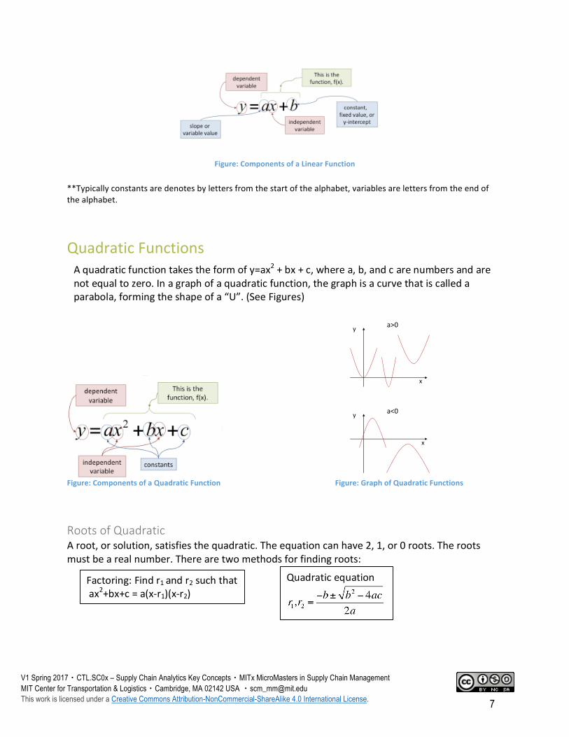
Figure:ComponentsofaLinearFunction**Typicallyconstantsaredenotesbylettersfromthestartofthealphabet,variablesarelettersfromtheendofthealphabet.
QuadraticFunctions
Figure:ComponentsofaQuadraticFunction Figure:GraphofQuadraticFunctions
RootsofQuadraticAroot,orsolution,satisfiesthequadratic.Theequationcanhave2,1,or0roots.Therootsmustbearealnumber.Therearetwomethodsforfindingroots:
Quadratic Functions
• When a>0, the function is convex (or concave up)• When a<0, the function is concave down
13
y =ax2 +bx+c
dependent variable
This is the function, f(x).
constantsindependent variable
Parabola - Polynomial function of degree 2 where a, b, and c are numbers and a≠0
a>0
x
y
x
y a<0
Aquadraticfunctiontakestheformofy=ax2+bx+c,wherea,b,andcarenumbersandarenotequaltozero.Inagraphofaquadraticfunction,thegraphisacurvethatiscalledaparabola,formingtheshapeofa“U”.(SeeFigures)
Quadraticequation
Factoring:Findr1andr2suchthatax2+bx+c=a(x-r1)(x-r2)
Page 8
V1 Spring 2017・CTL.SC0x – Supply Chain Analytics Key Concepts・MITx MicroMasters in Supply Chain Management MIT Center for Transportation & Logistics・Cambridge, MA 02142 USA ・[email protected] This work is licensed under a Creative Commons Attribution-NonCommercial-ShareAlike 4.0 International License. 8
OtherCommonFunctionalFormsPowerFunctionApowerfunctionisafunctionwherea≠ zero,isaconstant,andbisarealnumber.Theshapeofthecurveisdictatedbythevalueofb.
y=f(x)=axbExponentialFunctionsExponentialfunctionshaveveryfastgrowth.Inexponentialfunctions,thevariableisthepower.
y=abx
MultivariateFunctionsFunctionwithmorethanoneindependentxvariable(x1,x2,x3).
ConvexityandContinuityPropertiesoffunctions:
• Convexity:Doesthefunction“holdwater”?• Continuity:Functioniscontinuousifyoucandrawitwithoutliftingpenfrompaper!
LearningObjectives• Recognizedecision-makingiscoretosupplychainmanagement.• Gainperspectivesonwhentouseanalyticalmodels.• Understandbuildingblocksthatserveasthefoundationtoanalyticalmodels.
Euler’snumber,ore,isaconstantnumberthatisthebaseofthenaturallogarithm.e=2.7182818…
Y=ex
Logarithms:Alogarithmisaquantityrepresentingthepowertowhichafixednumbermustberaisedtoproduceagivennumber.Itistheinversefunctionofanexponential.
Page 9
V1 Spring 2017・CTL.SC0x – Supply Chain Analytics Key Concepts・MITx MicroMasters in Supply Chain Management MIT Center for Transportation & Logistics・Cambridge, MA 02142 USA ・[email protected] This work is licensed under a Creative Commons Attribution-NonCommercial-ShareAlike 4.0 International License. 9
Optimization
SummaryThisisanintroductionandoverviewofoptimization.Itstartswithanoverviewofunconstrainedoptimizationandhowtofindextremepointsolutions,keepinginmindfirstorderandsecondorderconditions.Italsoreviewsrulesinfunctionssuchasthepowerrule.Nextthelessonreviewconstrainedoptimizationthatsharessimilarobjectivesofunconstrainedoptimizationbutaddsadditionaldecisionvariablesandconstraintsonresources.Tosolveconstrainedoptimizationproblems,thelessonintroducesmathematicalprogramsthatarewidelyusedinsupplychainformanypracticessuchasdesigningnetworks,planningproduction,selectingtransportationproviders,allocatinginventory,schedulingportandterminaloperations,fulfillingorders,etc.Theoverviewoflinearprogrammingincludeshowtoformulatetheproblem,howtographicallyrepresentthem,andhowtoanalyzethesolutionandconductasensitivityanalysis.Inrealsupplychains,youcannot.5bananasinanorderorshipment.Thismeansthatwemustaddadditionalconstraintsforintegerprogrammingwhereeitherallofthedecisionvariablesmustbeintegers,orinamixedintegerprogrammingwheresome,butnotall,variablesarerestrictedtobeaninteger.Wereviewthetypesofnumbersyouwillencounter.Thenweintroduceintegerprogramsandhowtheyaredifferent.Wethenreviewthestepstoformulatinganintegerprogramandconcludewithconditionsforworkingwithbinaryvariables.
KeyConcepts
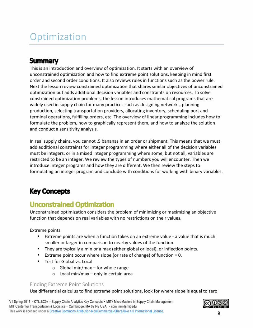
UnconstrainedOptimizationUnconstrainedoptimizationconsiderstheproblemofminimizingormaximizinganobjectivefunctionthatdependsonrealvariableswithnorestrictionsontheirvalues.Extremepoints
• Extremepointsarewhenafunctiontakesonanextremevalue-avaluethatismuchsmallerorlargerincomparisontonearbyvaluesofthefunction.
• Theyaretypicallyaminoramax(eitherglobalorlocal),orinflectionpoints.• Extremepointoccurwhereslope(orrateofchange)offunction=0.• TestforGlobalvs.Local
o Globalmin/max–forwholerangeo Localmin/max–onlyincertainarea
FindingExtremePointSolutionsUsedifferentialcalculustofindextremepointsolutions,lookforwhereslopeisequaltozero
Page 10
V1 Spring 2017・CTL.SC0x – Supply Chain Analytics Key Concepts・MITx MicroMasters in Supply Chain Management MIT Center for Transportation & Logistics・Cambridge, MA 02142 USA ・[email protected] This work is licensed under a Creative Commons Attribution-NonCommercial-ShareAlike 4.0 International License. 10
Tofindtheextremepoint,thereisathree-stepprocess:
1. Takethefirstderivativeofyourfunction2. Setitequaltozero,and3. SolveforX*,thevalueofxatextremepoint.
ThisiscalledtheFirstOrderCondition.Instantaneousslope(orfirstderivative)occurswhen:
• dy/dxisthecommonform,wheredmeanstherateofchange.
TheProductRule:Iffunctionisconstant,itdoesn’thaveanyeffect.
y = f (x) = a à y ' = f '(x) = 0 PowerRuleiscommonlyusedforfindingderivativesofcomplexfunctions.
y = f (x) = axn à y ' = f '(x) = anxn−1
FirstandSecondOrderConditionsInordertodeterminex*atthemax/minofanunconstrainedfunction
• FirstOrder(necessary)condition–theslopemustbe0f’(x*)=0
• Secondorder(sufficiency)condition-determineswhereextremepointisminormaxbytakingthesecondderivative,f”(x).
o Iff”(x)>0extremepointisalocalmino Iff”(x)<0extremepointisalocalmaxo Iff”(x)=0itisinconclusive
• Specialcaseso Iff(x)isconvex–>globalmino Iff(x)isconcave–>globalmax
δ (delta)=rateofchange.
Page 11
V1 Spring 2017・CTL.SC0x – Supply Chain Analytics Key Concepts・MITx MicroMasters in Supply Chain Management MIT Center for Transportation & Logistics・Cambridge, MA 02142 USA ・[email protected] This work is licensed under a Creative Commons Attribution-NonCommercial-ShareAlike 4.0 International License. 11
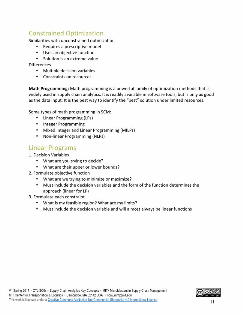
ConstrainedOptimizationSimilaritieswithunconstrainedoptimization
• Requiresaprescriptivemodel• Usesanobjectivefunction• Solutionisanextremevalue
Differences• Multipledecisionvariables• Constraintsonresources
MathProgramming:Mathprogrammingisapowerfulfamilyofoptimizationmethodsthatiswidelyusedinsupplychainanalytics.Itisreadilyavailableinsoftwaretools,butisonlyasgoodasthedatainput.Itisthebestwaytoidentifythe“best”solutionunderlimitedresources.SometypesofmathprogramminginSCM:
• LinearProgramming(LPs)• IntegerProgramming• MixedIntegerandLinearProgramming(MILPs)• Non-linearProgramming(NLPs)
LinearPrograms1.DecisionVariables
• Whatareyoutryingtodecide?• Whataretheirupperorlowerbounds?
2.Formulateobjectivefunction• Whatarewetryingtominimizeormaximize?• Mustincludethedecisionvariablesandtheformofthefunctiondeterminesthe
approach(linearforLP)3.Formulateeachconstraint
• Whatismyfeasibleregion?Whataremylimits?• Mustincludethedecisionvariableandwillalmostalwaysbelinearfunctions
Page 12
V1 Spring 2017・CTL.SC0x – Supply Chain Analytics Key Concepts・MITx MicroMasters in Supply Chain Management MIT Center for Transportation & Logistics・Cambridge, MA 02142 USA ・[email protected] This work is licensed under a Creative Commons Attribution-NonCommercial-ShareAlike 4.0 International License. 12
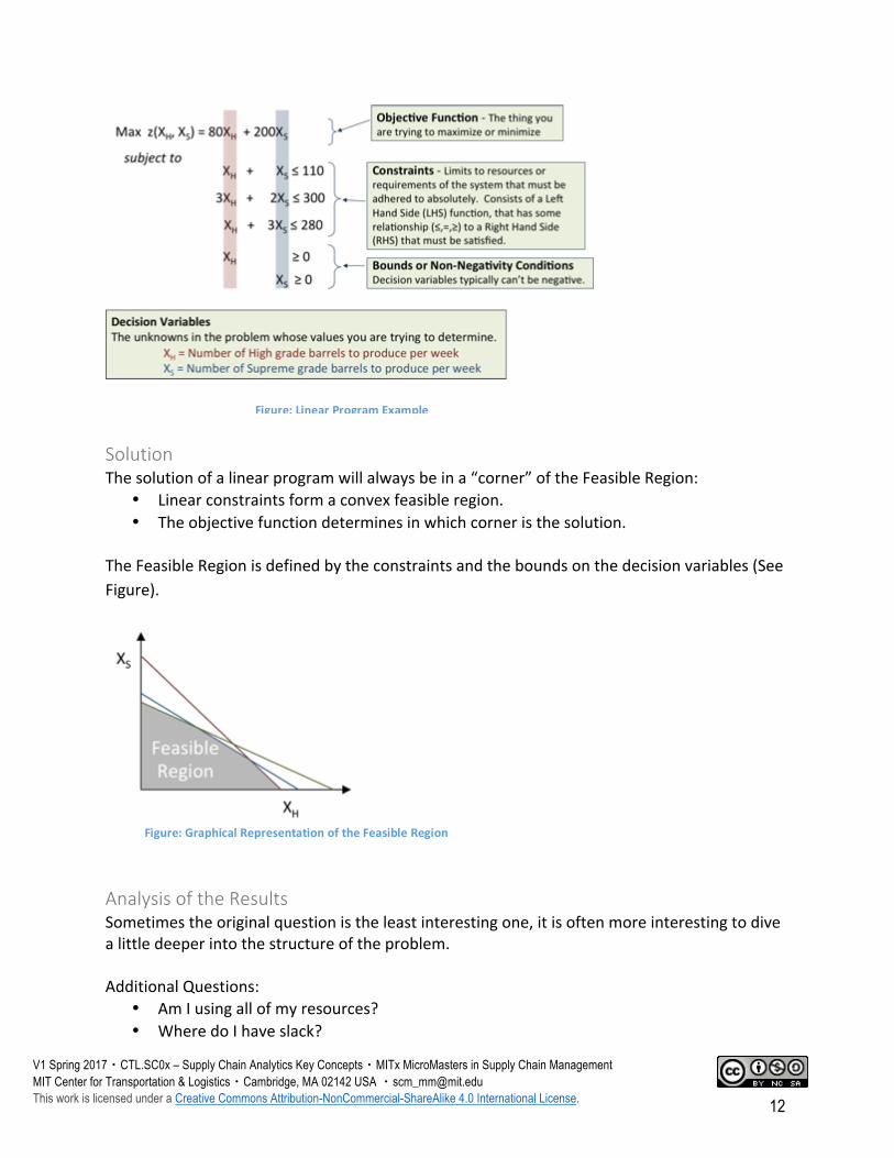
SolutionThesolutionofalinearprogramwillalwaysbeina“corner”oftheFeasibleRegion:
• Linearconstraintsformaconvexfeasibleregion.• Theobjectivefunctiondeterminesinwhichcorneristhesolution.
TheFeasibleRegionisdefinedbytheconstraintsandtheboundsonthedecisionvariables(SeeFigure).
AnalysisoftheResultsSometimestheoriginalquestionistheleastinterestingone,itisoftenmoreinterestingtodivealittledeeperintothestructureoftheproblem.AdditionalQuestions:
• AmIusingallofmyresources?• WheredoIhaveslack?
Figure:LinearProgramExample
Figure:GraphicalRepresentationoftheFeasibleRegion
Page 13
V1 Spring 2017・CTL.SC0x – Supply Chain Analytics Key Concepts・MITx MicroMasters in Supply Chain Management MIT Center for Transportation & Logistics・Cambridge, MA 02142 USA ・[email protected] This work is licensed under a Creative Commons Attribution-NonCommercial-ShareAlike 4.0 International License. 13
• WhereIamconstrained?• Howrobustismysolution?
SensitivityAnalysis:whathappenswhendatavaluesarechanged.
• ShadowPriceorDualValueofConstraint:Whatisthemarginalgainintheprofitabilityforanincreaseofoneontherighthandsideoftheconstraint?
• SlackConstraint–Foragivensolution,aconstraintisnotbindingiftotalvalueofthelefthandsideisnotequaltotherighthandsidevalue.Otherwiseitisabindingconstraint
• BindingConstraint–Aconstraintisbindingifchangingitalsochangestheoptimalsolution
AnomaliesinLinearProgramming
• AlternativeorMultipleOptimalSolutions(seeFigure)
• RedundantConstraints-DoesnoteffecttheFeasibleRegion;itisredundant.• Infeasibility-TherearenopointsintheFeasibleRegion;constraintsmaketheproblem
infeasible.
Figure:AlternativeofMultipleOptimalSolutions
Page 14
V1 Spring 2017・CTL.SC0x – Supply Chain Analytics Key Concepts・MITx MicroMasters in Supply Chain Management MIT Center for Transportation & Logistics・Cambridge, MA 02142 USA ・[email protected] This work is licensed under a Creative Commons Attribution-NonCommercial-ShareAlike 4.0 International License. 14
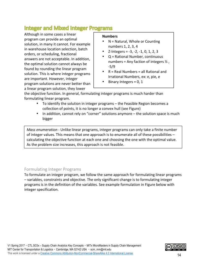
IntegerandMixedIntegerProgramsAlthoughinsomecasesalinearprogramcanprovideanoptimalsolution,inmanyitcannot.Forexampleinwarehouselocationselection,batchorders,orscheduling,fractionalanswersarenotacceptable.Inaddition,theoptimalsolutioncannotalwaysbefoundbyroundingthelinearprogramsolution.Thisiswhereintegerprogramsareimportant.However,integerprogramsolutionsareneverbetterthanalinearprogramsolution,theylowertheobjectivefunction.Ingeneral,formulatingintegerprogramsismuchharderthanformulatinglinearprogram.
• Toidentifythesolutioninintegerprograms–theFeasibleRegionbecomesacollectionofpoints,itisnolongeraconvexhull(seeFigure)
• Inaddition,cannotrelyon“corner”solutionsanymore–thesolutionspaceismuchbigger
FormulatingIntegerProgramsToformulateanintegerprogram,wefollowthesameapproachforformulatinglinearprograms–variables,constraintsandobjective.Theonlysignificantchangeistoformulatingintegerprogramsisinthedefinitionofthevariables.SeeexampleformulationinFigurebelowwithintegerspecification.
Numbers• N=Natural,WholeorCounting
numbers1,2,3,4• Z-Integers=-3,-2,-1,0,1,2,3• Q=RationalNumber,continuous
numbers=Anyfactionofintegers½,-5/9
• R=RealNumbers=allRationalandIrrationalNumbers,ex:e,pie,e
• BinaryIntegers=0,1
Massenumeration-Unlikelinearprograms,integerprogramscanonlytakeafinitenumberofintegervalues.Thismeansthatoneapproachistoenumerateallofthesepossibilities–calculatingtheobjectivefunctionateachoneandchoosingtheonewiththeoptimalvalue.Astheproblemsizeincreases,thisapproachisnotfeasible.
Page 15
V1 Spring 2017・CTL.SC0x – Supply Chain Analytics Key Concepts・MITx MicroMasters in Supply Chain Management MIT Center for Transportation & Logistics・Cambridge, MA 02142 USA ・[email protected] This work is licensed under a Creative Commons Attribution-NonCommercial-ShareAlike 4.0 International License. 15
BinaryVariablesSupposeyouhadthefollowingformulationofaminimizationproblemsubjecttocapacityatplantsandmeetingdemandforindividualproducts:
Wecouldaddbinaryvariablestothisformulationtobeabletomodelseveraldifferentlogicalconditions.Binaryvariablesareintegervariablesthatcanonlytakethevaluesof0or1.Generally,apositivedecision(dosomething)isrepresentedby1andthenegativedecision(donothing)isrepresentedbythevalueof0.Introducingabinaryvariabletothisformulation,wewouldhave:
Min z = cij xijj∑i∑s.t.
xiji∑ ≤C j ∀j
xijj∑ ≥ Di ∀i
xij ≥ 0 ∀ij
Maxz(XHL,XSL)=8XHL+20XSL
XHL+XSL≤11
3XHL+2XSL≤30
XHL+3XSL≤28
XHL,XSL≥0Integers
s.t.
Plant
Add.A
Add.B
Figure:Formulatinganintegerprogram
where:xij=Numberofunitsofproductimadeinplantjcij=CostperunitofproductimadeatplantjCj=CapacityinunitsatplantjDi=Demandforproductiinunits
Page 16
V1 Spring 2017・CTL.SC0x – Supply Chain Analytics Key Concepts・MITx MicroMasters in Supply Chain Management MIT Center for Transportation & Logistics・Cambridge, MA 02142 USA ・[email protected] This work is licensed under a Creative Commons Attribution-NonCommercial-ShareAlike 4.0 International License. 16
Notethatthenotonlywehaveaddedthebinaryvariableintheobjectivefunction,wehavealsoaddedanewconstraint(thethirdone).Thisisknownasalinkingconstraintoralogicalconstraint.Itisrequiredtoenforceanif-thenconditioninthemodel.Anypositivevalueofxijwillforcetheyjvariabletobeequaltoone.The“M”valueisabignumber–itshouldbeassmallaspossible,butatleastasbigasthevaluesofwhatsumofthexij’scanbe.Therearealsomoretechnicaltricksthatcanbeusedtotightenthisformulation.WecanalsointroduceEither/OrConditions-wherethereisachoicebetweentwoconstraints,onlyoneofwhichhastohold;itensuresaminimumlevel,Lj,ifyj=1.
xiji∑ −My j ≤ 0 ∀j xiji∑ − Lj y j ≥ 0 ∀j
Forexample:xiji∑ ≤C j ∀j
xijj∑ ≥ Di ∀i
xiji∑ −My j ≤ 0 ∀j
WeneedtoaddaconstraintthatensuresthatifweDOuseplantj,thatthevolumeisbetweentheminimumallowablelevel,Lj,andthemaximumcapacity,Cj.ThisissometimescalledanEither-Orcondition.
Min z = cij xijj∑i∑ + f j y jj∑s.t.
xiji∑ ≤C j ∀j
xijj∑ ≥ Di ∀i
xiji∑ −My j ≤ 0 ∀j
xij ≥ 0 ∀ij
y j ={0,1}
where:xij=Numberofunitsofproductimadeinplantjyj=1ifplantjisopened;=0otherwisecij=Costperunitofproductimadeatplantjfj=FixedcostforproducingatplantjCj=CapacityinunitsatplantjDi=Demandforproductiinunits M=abignumber(suchasCjinthiscase)
where: xij=Numberofunitsofproductimadeinplantj yj=1ifplantjisopened;=0o.w. M=abignumber(suchasCjinthiscase) Cj=Maximumcapacityinunitsatplantj Lj=Minimumlevelofproductionatplantj Di=Demandforproductiinunits
Page 17
V1 Spring 2017・CTL.SC0x – Supply Chain Analytics Key Concepts・MITx MicroMasters in Supply Chain Management MIT Center for Transportation & Logistics・Cambridge, MA 02142 USA ・[email protected] This work is licensed under a Creative Commons Attribution-NonCommercial-ShareAlike 4.0 International License. 17
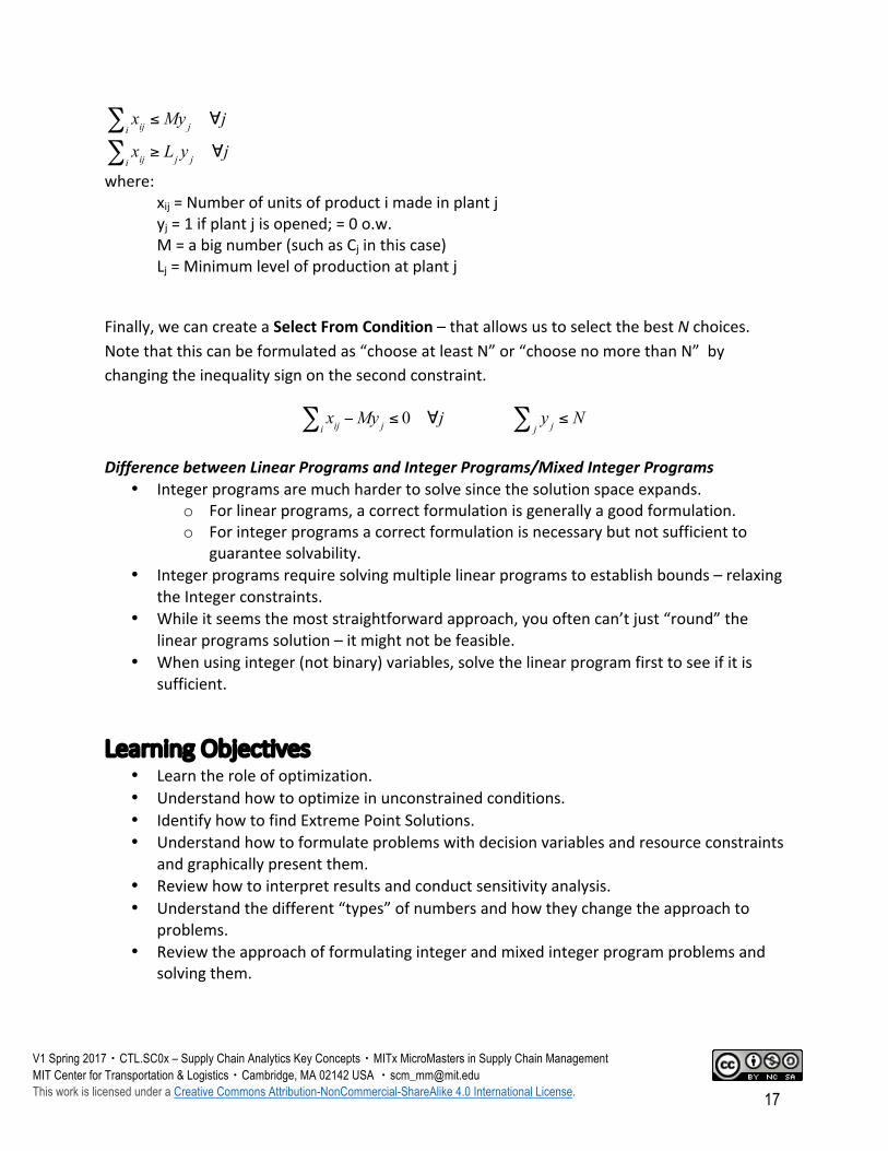
xiji∑ ≤My j ∀j
xiji∑ ≥ Lj y j ∀j
where: xij=Numberofunitsofproductimadeinplantj yj=1ifplantjisopened;=0o.w. M=abignumber(suchasCjinthiscase) Lj=Minimumlevelofproductionatplantj
Finally,wecancreateaSelectFromCondition–thatallowsustoselectthebestNchoices.Notethatthiscanbeformulatedas“chooseatleastN”or“choosenomorethanN”bychangingtheinequalitysignonthesecondconstraint.
xiji∑ −My j ≤ 0 ∀j y jj∑ ≤ N
DifferencebetweenLinearProgramsandIntegerPrograms/MixedIntegerPrograms• Integerprogramsaremuchhardertosolvesincethesolutionspaceexpands.
o Forlinearprograms,acorrectformulationisgenerallyagoodformulation.o Forintegerprogramsacorrectformulationisnecessarybutnotsufficientto
guaranteesolvability.• Integerprogramsrequiresolvingmultiplelinearprogramstoestablishbounds–relaxing
theIntegerconstraints.• Whileitseemsthemoststraightforwardapproach,youoftencan’tjust“round”the
linearprogramssolution–itmightnotbefeasible.• Whenusinginteger(notbinary)variables,solvethelinearprogramfirsttoseeifitis
sufficient.
LearningObjectives• Learntheroleofoptimization.• Understandhowtooptimizeinunconstrainedconditions.• IdentifyhowtofindExtremePointSolutions.• Understandhowtoformulateproblemswithdecisionvariablesandresourceconstraints
andgraphicallypresentthem.• Reviewhowtointerpretresultsandconductsensitivityanalysis.• Understandthedifferent“types”ofnumbersandhowtheychangetheapproachto
problems.• Reviewtheapproachofformulatingintegerandmixedintegerprogramproblemsand
solvingthem.
Page 18
V1 Spring 2017・CTL.SC0x – Supply Chain Analytics Key Concepts・MITx MicroMasters in Supply Chain Management MIT Center for Transportation & Logistics・Cambridge, MA 02142 USA ・[email protected] This work is licensed under a Creative Commons Attribution-NonCommercial-ShareAlike 4.0 International License. 18
AdvancedOptimization
SummaryThisreviewconcludesthelearningportiononoptimizationwithanoverviewofsomefrequentlyusedadvancedoptimizationmodels.Networkmodelsarekeyforsupplychainprofessionals.Thereviewbeginsbyfirstdefiningtheterminologyusedfrequentlyinthesenetworks.ItthenintroducescommonnetworkproblemsincludingtheShortestPath,TravelingSalesmanProblem(TSP),andFlowproblems.Theseareusedfrequentinsupplychainmanagementandunderstandingwhentheyariseandhowtosolvethemisessential.Wethenintroducenon-linearoptimization,highlightingitsdifferenceswithlinearprogramming,andanoverviewofhowtosolvenon-linearproblems.Thereviewconcludeswithpracticalrecommendationsofforconductingoptimization,emphasizingthatsupplychainprofessionalsshould:knowtheirproblem,theirteamandtheirtool.
KeyConcepts
NetworkModelsNetworkTerminology
• Nodeorvertices–apoint(facility,DC,plant,region)• Arcoredge–linkbetweentwonodes(roads,flows,etc.)maybedirectional• Networkorgraph–acollectionofnodesandarcs
CommonNetworkProblemsShortestPath–Easy&fasttosolve(LPorspecialalgorithms)Resultofshortestpartproblemisusedasthebaseofalotofotheranalysis.Itconnectsphysicaltooperationalnetwork.
• Given:One,origin,onedestination.• Find:Shortestpathfromsingleorigintosingledestination,• Challenges:Timeordistance?Impactofcongestionorweather?Howfrequentlyshould
weupdatethenetwork?• Integralityisguaranteed.• Caveat:Otherspecializedalgorithmsleveragethenetworkstructuretosolvemuch
faster.TravelingSalesmanProblem(TSP)–Hardtosolve(heuristics)
• Given:Oneorigin,manydestinations,sequentialstops,onevehicle.• Objective:Startingfromanoriginnode,findtheminimumdistancerequiredtovisit
eachnodeonceandonlyoneandreturntotheorigin.
Page 19
V1 Spring 2017・CTL.SC0x – Supply Chain Analytics Key Concepts・MITx MicroMasters in Supply Chain Management MIT Center for Transportation & Logistics・Cambridge, MA 02142 USA ・[email protected] This work is licensed under a Creative Commons Attribution-NonCommercial-ShareAlike 4.0 International License. 19
• Importance:TSPisatthecoreofallvehicleroutingproblems;localroutingandlastmiledeliveriesarebothcommonandimportant.
• Challenges:Itisexceptionallyhardtosolveexactly,duetoitssize;possiblesolutionsincreaseexponentiallywithnumberofnodes.
• Primaryapproach:specialalgorithmsforexactsolutions(smallerproblems)–Heuristics(manyavailable).
o Twoexamples:NearestNeighbor,CheapestInsertion
FlowProblems(Transportation&Transshipment)–Widelyused(MILPs)• Given:Multiplesupplyanddemandnodeswithfixedcostsandcapacitiesonnodes
and/orarcs.• Objective:Findtheminimumcostflowofproductfromsupplynodesthatsatisfy
demandatdestinationnodes.• Importance:Transportationproblemsareeverywhere;transshipmentproblemsareat
theheartoflargersupplychainnetworkdesignmodels.Intransportationproblems,shipmentsarebetweentwonodes.Fortransshipmentproblems,shipmentsmaygothroughintermediarynodes,possiblychangingmodeoftransport.Transshipmentproblemscanbeconvertedintotransportationproblems.
• Challenges:datarequirementscanbeextensive;difficulttodrawthelineon“realism”vs.“practicality”.
• Primaryapproaches:mixedintegerlinearprograms;somesimulation–usuallyafteroptimization.
NearestNeighborHeuristicThisalgorithmstartswiththesalesmanatarandomcityandvisitsthenearestcityuntilallhavebeenvisited.Ityieldsashorttour,buttypicallynottheoptimalone.
• Selectanynodetobetheactivenode.
• Connecttheactivenodetotheclosestunconnectednode;makethatthenewactivenode.
• Iftherearemoreunconnectednodesgotostep2,otherwiseconnecttotheoriginandend.
CheapestInsertionHeuristicOneapproachtotheTSPistostartwithasubtour–tourofsmallsubsetsofnodes,andextendthistourbyinsertingtheremainingnodesoneaftertheotheruntilallnodeshavebeeninserted.Thereareseveraldecisionstobemadeinhowtoconstructtheinitialtour,howtochoosenextnodetobeinserted,wheretoinsertchosennode.
• Formasubtourfromtheconvexhull.
• Addtothetourtheunconnectednodethatincreasesthecosttheleast;continueuntilallnodesareconnected.
Page 20
V1 Spring 2017・CTL.SC0x – Supply Chain Analytics Key Concepts・MITx MicroMasters in Supply Chain Management MIT Center for Transportation & Logistics・Cambridge, MA 02142 USA ・[email protected] This work is licensed under a Creative Commons Attribution-NonCommercial-ShareAlike 4.0 International License. 20
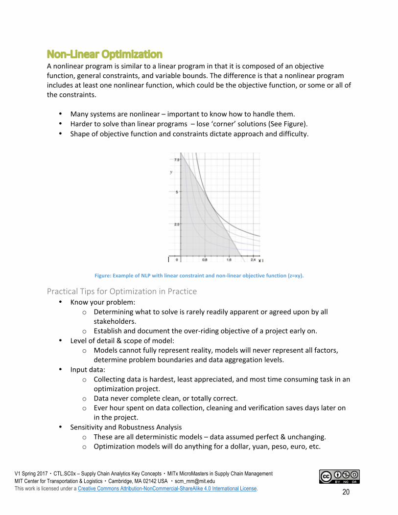
Non-LinearOptimizationAnonlinearprogramissimilartoalinearprograminthatitiscomposedofanobjectivefunction,generalconstraints,andvariablebounds.Thedifferenceisthatanonlinearprogramincludesatleastonenonlinearfunction,whichcouldbetheobjectivefunction,orsomeoralloftheconstraints.
• Manysystemsarenonlinear–importanttoknowhowtohandlethem.• Hardertosolvethanlinearprograms–lose‘corner’solutions(SeeFigure).• Shapeofobjectivefunctionandconstraintsdictateapproachanddifficulty.
Figure:ExampleofNLPwithlinearconstraintandnon-linearobjectivefunction(z=xy).
PracticalTipsforOptimizationinPractice• Knowyourproblem:
o Determiningwhattosolveisrarelyreadilyapparentoragreeduponbyallstakeholders.
o Establishanddocumenttheover-ridingobjectiveofaprojectearlyon.• Levelofdetail&scopeofmodel:
o Modelscannotfullyrepresentreality,modelswillneverrepresentallfactors,determineproblemboundariesanddataaggregationlevels.
• Inputdata:o Collectingdataishardest,leastappreciated,andmosttimeconsumingtaskinan
optimizationproject.o Datanevercompleteclean,ortotallycorrect.o Everhourspentondatacollection,cleaningandverificationsavesdayslateron
intheproject.• SensitivityandRobustnessAnalysis
o Thesearealldeterministicmodels–dataassumedperfect&unchanging.o Optimizationmodelswilldoanythingforadollar,yuan,peso,euro,etc.
Page 21
V1 Spring 2017・CTL.SC0x – Supply Chain Analytics Key Concepts・MITx MicroMasters in Supply Chain Management MIT Center for Transportation & Logistics・Cambridge, MA 02142 USA ・[email protected] This work is licensed under a Creative Commons Attribution-NonCommercial-ShareAlike 4.0 International License. 21
o Runmultiple“what-if”scenarioschanginguncertaininputvaluesandtestingdifferentconditions.
• Modelsvs.People(modelsdon’tmakedecisions,peopledo!)o Optimizationmodelsaregoodatmakingtrade-offsbetweencomplicated
optionsanduncoveringunexpectedinsightsandsolutions.o Peoplearegoodat:
§ Consideringintangibleandnon-quantifiablefactors,§ Identifyingunderlyingpatterns,and§ Miningpreviousexperienceandinsights.§ ModelsshouldbeusedforDecisionSUPPORTnotforthedecision.
LearningObjectives• Introductiontoadvancedoptimizationmethods.• Understandtheconditionsandwhentoapplynetworkmodels.• Differentiatenonlinearoptimizationandwhenitshouldbeused.• Reviewrecommendationsforrunningoptimizationinpractice–emphasizing
importanceofknowingtheproblem,teamandtool.
Page 22
V1 Spring 2017・CTL.SC0x – Supply Chain Analytics Key Concepts・MITx MicroMasters in Supply Chain Management MIT Center for Transportation & Logistics・Cambridge, MA 02142 USA ・[email protected] This work is licensed under a Creative Commons Attribution-NonCommercial-ShareAlike 4.0 International License. 22
Page 23
V1 Spring 2017・CTL.SC0x – Supply Chain Analytics Key Concepts・MITx MicroMasters in Supply Chain Management MIT Center for Transportation & Logistics・Cambridge, MA 02142 USA ・[email protected] This work is licensed under a Creative Commons Attribution-NonCommercial-ShareAlike 4.0 International License. 23
AlgorithmsandApproximations
SummaryInthislessonwewillbereviewingAlgorithmsandapproximations.Thefirsthalfofthelessonwillbeareviewofalgorithms–whichyoutechnicallyhavealreadybeintroducedto,butperhapsnotintheseterms.Wewillbereviewingthebasicsofalgorithms,theircomponents,andhowtheyareusedinoureverydayproblemsolving!TodemonstratethesewewillbelookingatafewcommonsupplychainproblemssuchastheShortestPathproblem,TravelingSalesmanProblem,andVehicleRoutingProblemwhileapplyingtheappropriatealgorithmtosolvethem.Inthisnextpartofthelesswewillbereviewingapproximations.Approximationsaregoodfirststepsinsolvingaproblembecausetheyrequireminimaldata,allowforfastsensitivityanalysis,andenablequickscopingofthesolutionspace.Recognizinghowtouseapproximationmethodsareimportantinsupplychainmanagementbecausecommonlyoptimalsolutionsrequirelargeamountsofdataandaretimeconsumingtosolve.Soifthatlevelofgranularityisnotneeded,approximationmethodscanprovideabasistoworkfromandtoseewhetherfurtheranalysisisneeded.
AlgorithmsAlgorithm-aprocessorsetofrulestobefollowedincalculationsorotherproblem-solvingoperations,especiallybyacomputer.DesiredPropertiesofanAlgorithm
• shouldbeunambiguous• requireadefinedsetofinputs• produceadefinedsetofoutputs• shouldterminateandproducearesult,alwaysstoppingafterafinitetime.
AlgorithmExample:find_maxInputs:
• L=arrayofNintegervariables• v(i)=valueoftheithvariableinthelist
Algorithm:1. setmax=0andi=12. selectitemiinthelist3. ifv(i)>max,thensetmax=v(i)4. ifi<N,thenseti=i+1andgotostep2,otherwisegotostep55. end
Output:
Page 24
V1 Spring 2017・CTL.SC0x – Supply Chain Analytics Key Concepts・MITx MicroMasters in Supply Chain Management MIT Center for Transportation & Logistics・Cambridge, MA 02142 USA ・[email protected] This work is licensed under a Creative Commons Attribution-NonCommercial-ShareAlike 4.0 International License. 24
maximumvalueinarrayL(max)
ShortestPathProblemObjective:FindtheshortestpathinanetworkbetweentwonodesImportance:Itsresultisusedasbaseforotheranalysis,andconnectsphysicaltooperationalnetworkPrimaryapproaches:
• StandardLinearProgramming(LP)• SpecializedAlgorithms(Dijkstra’sAlgorithm)
Minimize: cijj∑i∑ xij
Subject to:x jii∑ =1 ∀ j = s
x jii∑ − xiji∑ = 0 ∀ j ≠ s, j ≠ t
xiji∑ =1 ∀ j = t
xij ≥ 0
where: xij=Numberofunitsflowingfromnodeitonodej cij=Costperunitforflowfromnodeitonodej s=Sourcenode–whereflowstarts t=Terminalnode–whereflowendsDijkstra’sAlgorithmDjikstra'salgorithm(namedafteritsdiscover,E.W.Dijkstra)solvestheproblemoffindingtheshortestpathfromapointinagraph(thesource)toadestination.L(j)=lengthofpathfromsourcenodestonodejP(j)=precedingnodeforjintheshortestpathS(j)=1ifnodejhasbeenvisited,=0otherwised(ij)=distanceorcostfromnodeitonodejInputs:
• Connectedgraphwithnodesandarcswithpositivecosts,d(ij)• Source(s)andTerminal(t)nodes
Page 25
V1 Spring 2017・CTL.SC0x – Supply Chain Analytics Key Concepts・MITx MicroMasters in Supply Chain Management MIT Center for Transportation & Logistics・Cambridge, MA 02142 USA ・[email protected] This work is licensed under a Creative Commons Attribution-NonCommercial-ShareAlike 4.0 International License. 25
Algorithm:1. forallnodesingraph,setL()=∞,P()=Null,S()=02. setstoi,S(i)=1,andL(i)=03. Forallnodes,j,directlyconnected(adjacent)tonodei;ifL(j)>L(i)+d(ij),thensetL(j)=
L(i)+d(ij)andP(j)=i4. ForallnodeswhereS()=0,selectthenodewithlowestL()andsetittoi,setS(i)=15. Isthisnodet,theterminalnode?Ifso,gotoend.Ifnot,gotostep36. end–returnL(t)
Output:L(t)andParrayTofindpathfromstot,startattheend.
• FindP(t)–sayitisj• Ifj=sourcenode,stop,otherwise,findP(j)• keeptracingprecedingnodesuntilyoureachsourcenode
TravelingSalesmanProblem(TSP)Startingfromanoriginnode,findtheminimumdistancerequiredtovisiteachnodeonceandonlyonceandreturntotheorigin.NearestNeighborHeuristic
1. Selectanynodetobetheactivenode2. Connecttheactivenodetotheclosestunconnectednode,makethatthenewactive
node.3. Iftherearemoreunconnectednodesgotostep2,otherwiseconnecttothestarting
nodeandend.
2-OptHeuristic1. Identifypairsofarcs(i-jandk-l),whered(ij)+d(kl)>d(ik)+d(jl)–usuallywherethey
cross2. Selectthepairwiththelargestdifference,andre-connectthearcs(i-kandj-l)3. Continueuntiltherearenomorecrossedarcs.
VehicleRoutingProblemFindminimumcosttoursfromsingleorigintomultipledestinationswithvaryingdemandusingmultiplecapacitatedvehicles.
Page 26
V1 Spring 2017・CTL.SC0x – Supply Chain Analytics Key Concepts・MITx MicroMasters in Supply Chain Management MIT Center for Transportation & Logistics・Cambridge, MA 02142 USA ・[email protected] This work is licensed under a Creative Commons Attribution-NonCommercial-ShareAlike 4.0 International License. 26
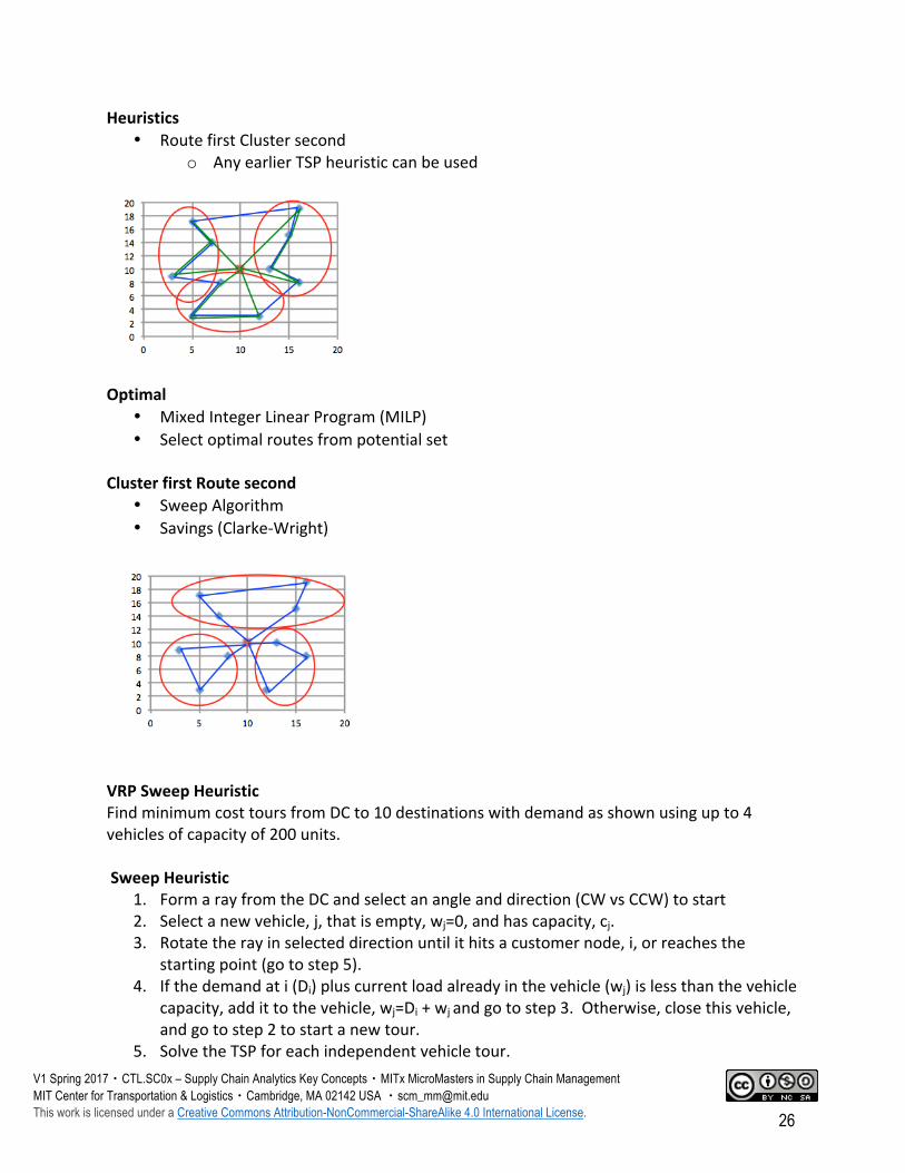
Heuristics• RoutefirstClustersecond
o AnyearlierTSPheuristiccanbeused
Optimal
• MixedIntegerLinearProgram(MILP)• Selectoptimalroutesfrompotentialset
ClusterfirstRoutesecond
• SweepAlgorithm• Savings(Clarke-Wright)
VRPSweepHeuristicFindminimumcosttoursfromDCto10destinationswithdemandasshownusingupto4vehiclesofcapacityof200units.SweepHeuristic
1. FormarayfromtheDCandselectanangleanddirection(CWvsCCW)tostart2. Selectanewvehicle,j,thatisempty,wj=0,andhascapacity,cj.3. Rotatetherayinselecteddirectionuntilithitsacustomernode,i,orreachesthe
startingpoint(gotostep5).4. Ifthedemandati(Di)pluscurrentloadalreadyinthevehicle(wj)islessthanthevehicle
capacity,addittothevehicle,wj=Di+wjandgotostep3.Otherwise,closethisvehicle,andgotostep2tostartanewtour.
5. SolvetheTSPforeachindependentvehicletour.
Page 27
V1 Spring 2017・CTL.SC0x – Supply Chain Analytics Key Concepts・MITx MicroMasters in Supply Chain Management MIT Center for Transportation & Logistics・Cambridge, MA 02142 USA ・[email protected] This work is licensed under a Creative Commons Attribution-NonCommercial-ShareAlike 4.0 International License. 27
Differentstartingpointsanddirectionscanyielddifferentsolutions!Besttouseavarietyorastackofheuristics.
Clark-WrightSavingsAlgorithmTheClarkeandWrightsavingsalgorithmisoneofthemostknownheuristicforVRP.Itappliestoproblemsforwhichthenumberofvehiclesisnotfixed(itisadecisionvariable)
• Startwithacompletesolution(outandback)• Identifynodestolinktoformacommontourbycalculatingthesavings:
Example:joiningnode1&2intoasingletour
Currenttourscost=2cO1+2cO2Joinedtourcosts=cO1+c12+c2O
So,if2cO1+2cO2>cO1+c12+c2OthenjointhemThatis:cO1+c2O–c12>0
• Thissavingsvaluecanbecalculatedforeverypairofnodes• Runthroughthenodespairingtheoneswiththehighestsavingsfirst• Needtomakesurevehiclecapacityisnotviolated• Also,“interiortour”nodescannotbeadded–mustbeonend
Page 28
V1 Spring 2017・CTL.SC0x – Supply Chain Analytics Key Concepts・MITx MicroMasters in Supply Chain Management MIT Center for Transportation & Logistics・Cambridge, MA 02142 USA ・[email protected] This work is licensed under a Creative Commons Attribution-NonCommercial-ShareAlike 4.0 International License. 28
SavingsHeuristic1. Calculatesavingssi,j=cO,i+cO,j-ci,jforeverypair(i,j)ofdemandnodes.2. Rankandprocessthesavingssi,jindescendingorderofmagnitude.3. Forthesavingssi,junderconsideration,includearc(i,j)inarouteonlyif:
• Norouteorvehicleconstraintswillbeviolatedbyaddingitinarouteand• Nodesiandjarefirstorlastnodesto/fromtheoriginintheircurrentroute.
4. Ifthesavingslisthasnotbeenexhausted,returntoStep3,processingthenextentryinthelist;otherwise,stop.
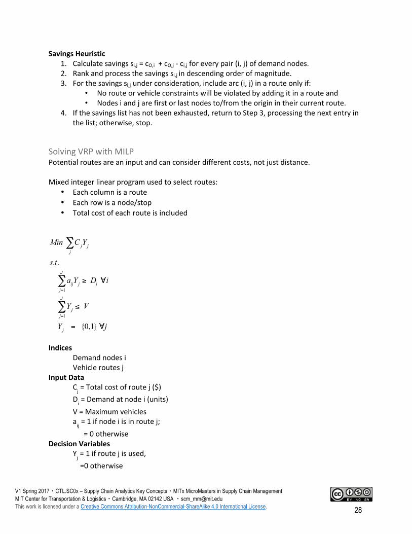
SolvingVRPwithMILPPotentialroutesareaninputandcanconsiderdifferentcosts,notjustdistance.Mixedintegerlinearprogramusedtoselectroutes:
• Eachcolumnisaroute• Eachrowisanode/stop• Totalcostofeachrouteisincluded
Min C jYjj∑
s.t.
aijY jj=1
J
∑ ≥ Di ∀i
Yjj=1
J
∑ ≤ V
Yj = {0,1} ∀j
Indices Demandnodesi VehicleroutesjInputData Cj=Totalcostofroutej($) Di=Demandatnodei(units) V=Maximumvehicles aij=1ifnodeiisinroutej; =0otherwiseDecisionVariables Yj=1ifroutejisused, =0otherwise
Page 29
V1 Spring 2017・CTL.SC0x – Supply Chain Analytics Key Concepts・MITx MicroMasters in Supply Chain Management MIT Center for Transportation & Logistics・Cambridge, MA 02142 USA ・[email protected] This work is licensed under a Creative Commons Attribution-NonCommercial-ShareAlike 4.0 International License. 29
ApproximationMethodsInthissecondhalfwewilldiscussexamplesofapproximationandestimation.InparticularwewillreviewestimationofOne-to-ManyDistributionthroughlinehauldistance,travelingsalesmanandvehicleroutingproblems.Approximation:avalueorquantitythatisnearlybutnotexactlycorrect.
Estimation:aroughcalculationofthevalue,number,quantity,orextentofsomething.synonyms:estimate,approximation,roughcalculation,roughguess,evaluation,back-of-theenvelope
Whyuseapproximationmethods?• Fasterthanmoreexactorprecisemethods,• Usesminimalamountsofdata,and• Candetermineifmoreanalysisisneeded:GoldilocksPrinciple:Toobig,Toolittle,Just
right.
Alwaystrytoestimateasolutionpriortoanalysis!
QuickEstimationSimpleEstimationRules:1.Breaktheproblemintopiecesthatyoucanestimateordeterminedirectly2.Estimateorcalculateeachpieceindependentlytowithinanorderofmagnitude3.CombinethepiecesbacktogetherpayingattentiontounitsExample:HowmanypianotunersarethereinChicago?"
• Thereareapproximately9,000,000peoplelivinginChicago.• Onaverage,therearetwopersonsineachhouseholdinChicago.• Roughlyonehouseholdintwentyhasapianothatistunedregularly.• Pianosthataretunedregularlyaretunedonaverageaboutonceperyear.• Ittakesapianotunerabouttwohourstotuneapiano,includingtraveltime.• Eachpianotunerworkseighthoursinaday,fivedaysinaweek,and50weeksinayear.
TuningsperYear=(9,000,000ppl)÷(2ppl/hh)×(1piano/20hh)×(1tuning/piano/year)=225,000TuningsperTunerperYear=(50wks/yr)×(5day/wk)×(8hrs/day)÷(2hrstotune)=1000NumberofPianoTuners=(225,000tuningsperyear)÷(1000tuningsperyearpertuner)=225ActualNumber=290
Page 30
V1 Spring 2017・CTL.SC0x – Supply Chain Analytics Key Concepts・MITx MicroMasters in Supply Chain Management MIT Center for Transportation & Logistics・Cambridge, MA 02142 USA ・[email protected] This work is licensed under a Creative Commons Attribution-NonCommercial-ShareAlike 4.0 International License. 30
EstimationofOnetoManyDistributionSingleDistributionCenter:
• Productsoriginatefromoneorigin• Productsaredemandedatmanydestinations• AlldestinationsarewithinaspecifiedServiceRegion• Ignoreinventory(samedaydelivery)
Assumptions:
• Vehiclesarehomogenous• Samecapacity,QMAX• Fleetsizeisconstant
Page 31
V1 Spring 2017・CTL.SC0x – Supply Chain Analytics Key Concepts・MITx MicroMasters in Supply Chain Management MIT Center for Transportation & Logistics・Cambridge, MA 02142 USA ・[email protected] This work is licensed under a Creative Commons Attribution-NonCommercial-ShareAlike 4.0 International License. 31
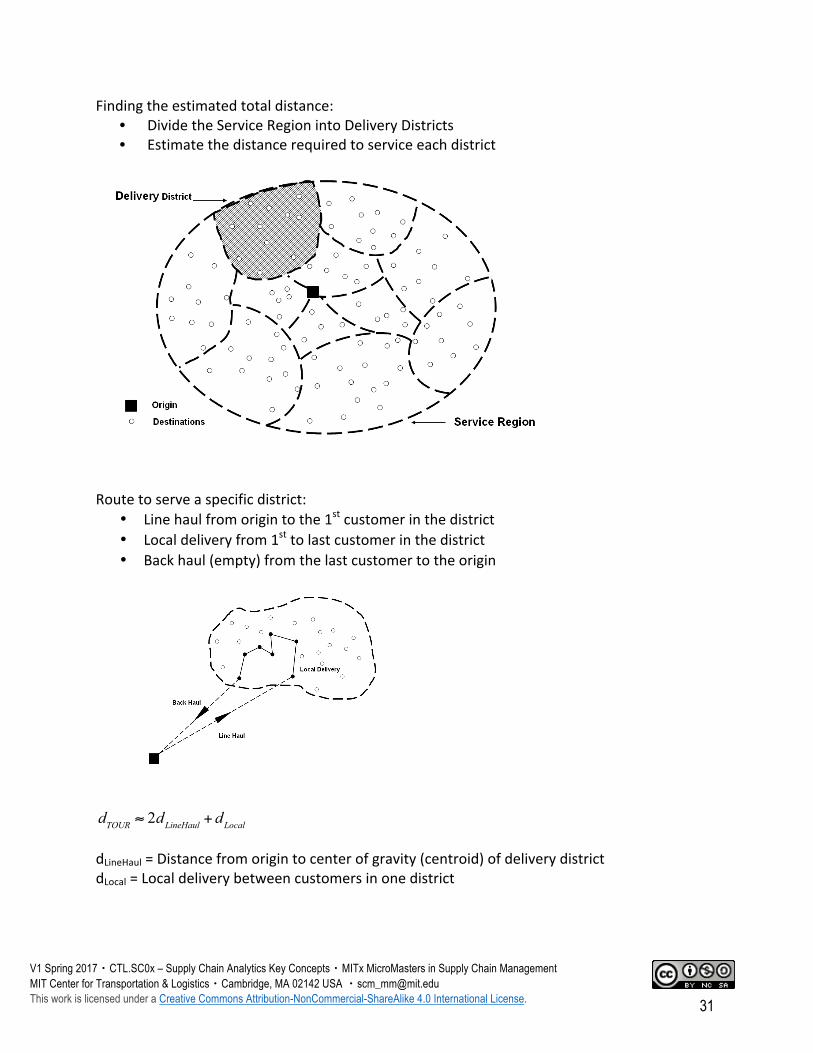
Findingtheestimatedtotaldistance:• DividetheServiceRegionintoDeliveryDistricts• Estimatethedistancerequiredtoserviceeachdistrict
Routetoserveaspecificdistrict:
• Linehaulfromorigintothe1stcustomerinthedistrict• Localdeliveryfrom1sttolastcustomerinthedistrict• Backhaul(empty)fromthelastcustomertotheorigin
dTOUR ≈ 2dLineHaul + dLocal
dLineHaul=Distancefromorigintocenterofgravity(centroid)ofdeliverydistrictdLocal=Localdeliverybetweencustomersinonedistrict
Page 32
V1 Spring 2017・CTL.SC0x – Supply Chain Analytics Key Concepts・MITx MicroMasters in Supply Chain Management MIT Center for Transportation & Logistics・Cambridge, MA 02142 USA ・[email protected] This work is licensed under a Creative Commons Attribution-NonCommercial-ShareAlike 4.0 International License. 32
Howdoweestimatedistances?• PointtoPoint• RoutingorwithinaTour
EstimatingPointtoPointDistancesDependsonthetopographyoftheunderlyingregionEuclideanSpace: dA-B=√[(xA-xB)2+(yA-yB)2]Grid: dA-B=|xA-xB|+|yA-yB|RandomNetwork:differentapproach
ForRandom(real)Networksuse:DA-B=kCFdA-BFinddA-B-the“ascrowflies”distance.
• Euclidean:forreallyshortdistanceso dA-B=SQRT((xA-xB)2+(yA-yB)2)
• GreatCircle:forlocationswithinthesamehemisphereo dA-B=3959(arccos[sin[LATA]sin[LATB]+cos[LATA]cos[LATB]cos[LONGA-LONGB]])
• Where:o LATi=Latitudeofpointiinradianso LONGi=Longitudeofpointiinradianso Radians=(AngleinDegrees)(π/180o)
Applyanappropriatecircuityfactor(kCF)
• Howdoyougetthisvalue?• Whatdoyouthinktherangesare?• Whataresomecautionsforthisapproach?
Page 33
V1 Spring 2017・CTL.SC0x – Supply Chain Analytics Key Concepts・MITx MicroMasters in Supply Chain Management MIT Center for Transportation & Logistics・Cambridge, MA 02142 USA ・[email protected] This work is licensed under a Creative Commons Attribution-NonCommercial-ShareAlike 4.0 International License. 33
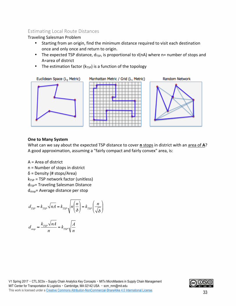
EstimatingLocalRouteDistancesTravelingSalesmanProblem
• Startingfromanorigin,findtheminimumdistancerequiredtovisiteachdestinationonceandonlyonceandreturntoorigin.
• TheexpectedTSPdistance,dTSP,isproportionalto√(nA)wheren=numberofstopsandA=areaofdistrict
• Theestimationfactor(kTSP)isafunctionofthetopology
OnetoManySystemWhatcanwesayabouttheexpectedTSPdistancetocovernstopsindistrictwithanareaofA?Agoodapproximation,assuminga"fairlycompactandfairlyconvex"area,is:A=Areaofdistrictn=Numberofstopsindistrictδ=Density(#stops/Area)kTSP=TSPnetworkfactor(unitless)dTSP=TravelingSalesmanDistancedstop=Averagedistanceperstop
dTSP ≈ kTSP nA = kTSP n nδ
⎛
⎝⎜⎞
⎠⎟ = kTSP
nδ
⎛
⎝⎜
⎞
⎠⎟
dstop ≈kTSP nAn
= kTSPAn
Page 34
V1 Spring 2017・CTL.SC0x – Supply Chain Analytics Key Concepts・MITx MicroMasters in Supply Chain Management MIT Center for Transportation & Logistics・Cambridge, MA 02142 USA ・[email protected] This work is licensed under a Creative Commons Attribution-NonCommercial-ShareAlike 4.0 International License. 34
WhatvaluesofkTSPshouldweuse?• LotsofresearchonthisforL1andL2networks-dependsondistrictshape,approachto
routing,etc.• Euclidean(L2)Networks
o kTSP=0.57to0.99dependingonclustering&sizeofN(MAPE~4%,MPE~-1%)o kTSP=0.765commonlyusedandisagoodapproximation!
• Grid(L1)Networkso kTSP=0.97to1.15dependingonclusteringandpartitioningofdistrict
EstimatingVehicleTourDistancesFindingthetotaldistancetraveledonalltours,where:
• l=numberoftours• c=numberofcustomerstopspertourand• n=totalnumberofstops=c*l
dTOUR = 2dLineHaul +ckTSPδ
dAllTours = ldTOUR = 2ldLineHaul +nkTSPδ
Minimizenumberoftoursbymaximizingvehiclecapacity
l = DQMAX
⎡
⎣⎢
⎤
⎦⎥
+
dAllTours = 2DQMAX
⎡
⎣⎢
⎤
⎦⎥
+
dLineHaul +nkTSPδ
[x]+=lowestintegervalue>x.ThisisastepfunctionEstimatethiswithcontinuousfunction: [x]+~x+½
Page 35
V1 Spring 2017・CTL.SC0x – Supply Chain Analytics Key Concepts・MITx MicroMasters in Supply Chain Management MIT Center for Transportation & Logistics・Cambridge, MA 02142 USA ・[email protected] This work is licensed under a Creative Commons Attribution-NonCommercial-ShareAlike 4.0 International License. 35
KeyPoints
• Reviewthebasisandcomponentsofalgorithms• Recognizedesiredpropertiesofanalgorithm• Reviewdifferentnetworkalgorithms• RecognizehowtosolvetheShortestPathProblem• RecognizewhichalgorithmstousefortheTravelingSalesmanProblem• RecognizehowtosolveaVehicleRoutingProblem(ClusterFirst–RouteSecond)• Reviewhowtouseapproximations• Recognizestepstoquickestimation
Page 36
V1 Spring 2017・CTL.SC0x – Supply Chain Analytics Key Concepts・MITx MicroMasters in Supply Chain Management MIT Center for Transportation & Logistics・Cambridge, MA 02142 USA ・[email protected] This work is licensed under a Creative Commons Attribution-NonCommercial-ShareAlike 4.0 International License. 36
DistributionsandProbability
SummaryWereviewtwoveryimportanttopicsinsupplychainmanagement:probabilityanddistributions.Probabilityisanoften-reoccurringthemeinsupplychainmanagementduetothecommonconditionsofuncertainty.Onagivenday,astoremightsell2unitsofaproduct,onanother,50.Toexplorethis,theprobabilityreviewincludesanintroductionofprobabilitytheory,probabilitylaws,andpropernotation.Summaryordescriptivestatisticsareshownforcapturingcentraltendencyandthedispersionofadistribution.Wealsointroducetwotheoreticaldiscretedistributions:UniformandPoisson.Wethenintroducethreecommoncontinuousdistributions:Uniform,Normal,andTriangle.Thereviewthengoesthroughthedifferencebetweendiscretevs.continuousdistributionsandhowtorecognizethesedifferences.Theremainderofthereviewisaexplorationintoeachtypeofdistribution,whattheylooklikegraphicallyandwhataretheprobabilitydensityfunctionandcumulativedensityfunctionofeach.
KeyConceptsProbabilityProbabilitydefinestheextenttowhichsomethingisprobable,orthelikelihoodofaneventhappening.Itismeasuredbytheratioofthecasetothetotalnumberofcasespossible.
ProbabilityTheory• Mathematicalframeworkforanalyzingrandomeventsorexperiments.• Experimentsareeventswecannotpredictwithcertainty(e.g.,weeklysalesatastore,
flippingacoin,drawingacardfromadeck,etc.).• Eventsareaspecificoutcomefromanexperiment(e.g.,sellinglessthan10itemsina
week,getting3headsinarow,drawingaredcard,etc.)
Page 37
V1 Spring 2017・CTL.SC0x – Supply Chain Analytics Key Concepts・MITx MicroMasters in Supply Chain Management MIT Center for Transportation & Logistics・Cambridge, MA 02142 USA ・[email protected] This work is licensed under a Creative Commons Attribution-NonCommercial-ShareAlike 4.0 International License. 37
ProbabilityLaws1.Theprobabilityofanyeventisbetween0and1,thatis0≤P(A)≤12.IfAandBaremutuallyexclusiveevents,thenP(AorB)=P(AUB)=P(A)+P(B)3.IfAandBareanytwoevents,then
P(A | B) = P(A and B)P(B)
=P A∩B( )P(B)
WhereP(AIB)istheconditionalprobabilityofAoccurringgivenBhasalreadyoccurred.4.IfAandBareindependentevents,then
P(A | B) = P(A)
P(A and B) = P(A∩B) = P A | B( )P(B) = P A( )×P B( )
WhereeventsAandBareindependentifknowingthatBoccurreddoesnotinfluencetheprobabilityofAoccurring.
SummarystatisticsDescriptiveorsummarystatisticsplayasignificantroleintheinterpretation,presentation,andorganizationofdata.Itcharacterizesasetofdata.Therearemanywaysthatwecancharacterizeadataset,wefocusedontwo:CentralTendencyandDispersionorSpread.
CentralTendencyThisis,inroughterms,the“mostlikely”valueofthedistribution.Itcanbeformallymeasuredinanumberofdifferentwaystoinclude:
• Mode–thespecificvaluethatappearsmostfrequently• Median–thevalueinthe“middle”ofadistributionthatseparatesthelowerfromthe
higherhalf.Thisisalsocalledthe50thpercentilevalue.• Mean(μ)–thesumofvaluesmultipliedbytheirprobability(calledtheexpectedvalue).
Thisisalsothesumofvaluesdividedbythetotalnumberofobservations(calledtheaverage).
Notation• P(A)–theprobabilitythateventAoccurs• P(A’)=complementofP(A)–probabilitysomeothereventthatisnotAoccurs.This
isalsotheprobabilitythatsomethingotherthanAhappens.
Page 38
V1 Spring 2017・CTL.SC0x – Supply Chain Analytics Key Concepts・MITx MicroMasters in Supply Chain Management MIT Center for Transportation & Logistics・Cambridge, MA 02142 USA ・[email protected] This work is licensed under a Creative Commons Attribution-NonCommercial-ShareAlike 4.0 International License. 38
E[X]= x = µ = pixii=1
n∑
Page 39
V1 Spring 2017・CTL.SC0x – Supply Chain Analytics Key Concepts・MITx MicroMasters in Supply Chain Management MIT Center for Transportation & Logistics・Cambridge, MA 02142 USA ・[email protected] This work is licensed under a Creative Commons Attribution-NonCommercial-ShareAlike 4.0 International License. 39
DispersionorSpreadThiscapturesthedegreetowhichtheobservations“differ”fromeachother.Themorecommondispersionmetricsare:
• Range–themaximumvalueminustheminimumvalue.• InnerQuartiles–75thpercentilevalueminusthe25thpercentilevalue-capturesthe
“centralhalf”oftheentiredistribution.• Variance(σ2)–theexpectedvalueofthesquareddeviationaroundthemean;also
calledtheSecondMomentaroundthemean
Var[X]=σ 2 = pi xi − x( )i=1
n∑
2= pi xi −µ( )
i=1
n∑
2
• StandardDeviation(σ)–thesquarerootofthevariance.Thisputsitinthesameunitsastheexpectedvalueormean.
• CoefficientofVariation(CV)–theratioofthestandarddeviationoverthemean=σ/μ.Thisisacommoncomparablemetricofdispersionacrossdifferentdistributions.Asageneralrule:
o 0≤CV≤0.75,lowvariabilityo 0.75≤CV≤1.33,moderatevariabilityo CV>1.33,highvariability
PopulationversusSampleVarianceInpractice,weusuallydonotknowthetruemeanofapopulation.Instead,weneedtoestimatethemeanfromasampleofdatapulledfromthepopulation.Whencalculatingthevariance,itisimportanttoknowwhetherweareusingallofthedatafromtheentirepopulationorjustusingasampleofthepopulation’sdata.Inthefirstcasewewanttofindthepopulationvariancewhileinthesecondcasewewanttofindthesamplevariance.Theonlydifferencesbetweencalculatingthepopulationversusthesamplevariances(andthustheircorrespondingstandarddeviations)isthatforthepopulationvariance,σ2,wedividethesumoftheobservationsbyn(thenumberofobservations)whileforthesamplevariance,s2,wedividebyn-1.
σ 2 =xi −µ( )
i=1
n∑
2
ns2 =
xi − x( )i=1
n∑
2
n−1
Notethatthesamplevariancewillbeslightlylargerthanthepopulationvarianceforsmallvaluesofn.Asngetslarger,thisdifferenceessentiallydisappears.Thereasonfortheusen-1isduetohavingtouseadegreeoffreedomincalculatingtheaverage(xbar)fromthesamesamplethatweareestimatingthevariance.Itleadstoanunbiasedestimateofthepopulationvariance.Inpractice,youshouldjustusethesamplevarianceandstandarddeviationunlessyouaredealingwithspecificprobabilities,likeflippingacoin.
Page 40
V1 Spring 2017・CTL.SC0x – Supply Chain Analytics Key Concepts・MITx MicroMasters in Supply Chain Management MIT Center for Transportation & Logistics・Cambridge, MA 02142 USA ・[email protected] This work is licensed under a Creative Commons Attribution-NonCommercial-ShareAlike 4.0 International License. 40
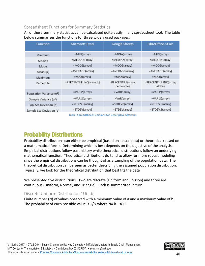
SpreadsheetFunctionsforSummaryStatisticsAllofthesesummarystatisticscanbecalculatedquiteeasilyinanyspreadsheettool.Thetablebelowsummarizesthefunctionsforthreewidelyusedpackages.
Table:SpreadsheetFunctionsforDescriptiveStatistics
ProbabilityDistributionsProbabilitydistributionscaneitherbeempirical(basedonactualdata)ortheoretical(basedonamathematicalform).Determiningwhichisbestdependsontheobjectiveoftheanalysis.Empiricaldistributionsfollowpasthistorywhiletheoreticaldistributionsfollowanunderlyingmathematicalfunction.Theoreticaldistributionsdotendtoallowformorerobustmodelingsincetheempiricaldistributionscanbethoughtofasasamplingofthepopulationdata.Thetheoreticaldistributioncanbeseenasbetterdescribingtheassumedpopulationdistribution.Typically,welookforthetheoreticaldistributionthatbestfitsthedataWepresentedfivedistributions.Twoarediscrete(UniformandPoisson)andthreearecontinuous(Uniform,Normal,andTriangle).Eachissummarizedinturn.
DiscreteUniformDistribution~U(a,b)Finitenumber(N)ofvaluesobservedwithaminimumvalueofaandamaximumvalueofb.Theprobabilityofeachpossiblevalueis1/NwhereN=b–a+1
Page 41
V1 Spring 2017・CTL.SC0x – Supply Chain Analytics Key Concepts・MITx MicroMasters in Supply Chain Management MIT Center for Transportation & Logistics・Cambridge, MA 02142 USA ・[email protected] This work is licensed under a Creative Commons Attribution-NonCommercial-ShareAlike 4.0 International License. 41
PoissonDistribution~P(λ)Discretefrequencydistributionthatgivestheprobabilityofanumberofindependenteventsoccurringinafixedtimewheretheparameterλ =mean=variance.Widelyusedtomodelarrivals,slowmovinginventory,etc.Notethatthedistributiononlycontainsnon-negativeintegersandcancapturenon-symmetricdistributions.Asthenumberofobservationsincrease,thedistributionbecomes“belllike”andapproximatestheNormalDistribution.
Table:SpreadsheetFunctionsforPoissondistribution
SummaryMetrics• Mean=λ• Median≈ ⎣(λ + 1/3 – 0.02/λ)⎦• Mode=⎣λ⎦• Variance=λ
ProbabilityMassFunction(pmf):
where• e=Euler’snumber~2.71828...• λ=meanvalue(parameter)• x!=factorialofx,e.g.,3!=3×2×1=6and0!=1
ProbabilityMassFunction(pmf):
SummaryMetrics• Mean=(a+b)/2• Median=(a+b)/2• ModeN/A(allvaluesareequallylikely)• Variance=((b-a+1)2-1)/12
Page 42
V1 Spring 2017・CTL.SC0x – Supply Chain Analytics Key Concepts・MITx MicroMasters in Supply Chain Management MIT Center for Transportation & Logistics・Cambridge, MA 02142 USA ・[email protected] This work is licensed under a Creative Commons Attribution-NonCommercial-ShareAlike 4.0 International License. 42
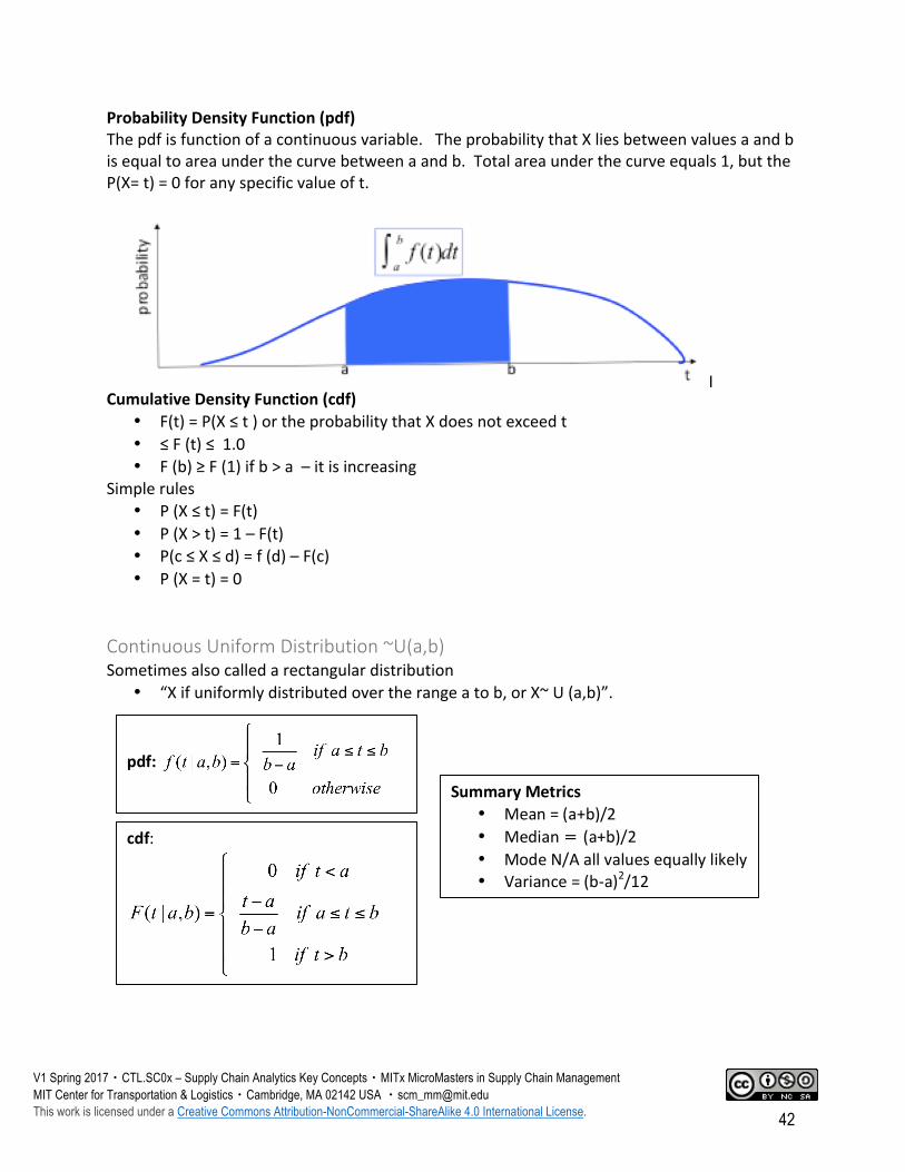
ProbabilityDensityFunction(pdf)Thepdfisfunctionofacontinuousvariable.TheprobabilitythatXliesbetweenvaluesaandbisequaltoareaunderthecurvebetweenaandb.Totalareaunderthecurveequals1,buttheP(X=t)=0foranyspecificvalueoft.
CumulativeDensityFunction(cdf)
• F(t)=P(X≤t)ortheprobabilitythatXdoesnotexceedt• ≤F(t)≤1.0• F(b)≥F(1)ifb>a–itisincreasing
Simplerules• P(X≤t)=F(t)• P(X>t)=1–F(t)• P(c≤X≤d)=f(d)–F(c)• P(X=t)=0
ContinuousUniformDistribution~U(a,b)Sometimesalsocalledarectangulardistribution
• “Xifuniformlydistributedovertherangeatob,orX~U(a,b)”.
pdf:
SummaryMetrics• Mean=(a+b)/2• Median= (a+b)/2• ModeN/Aallvaluesequallylikely• Variance=(b-a)2/12
cdf:
Page 43
V1 Spring 2017・CTL.SC0x – Supply Chain Analytics Key Concepts・MITx MicroMasters in Supply Chain Management MIT Center for Transportation & Logistics・Cambridge, MA 02142 USA ・[email protected] This work is licensed under a Creative Commons Attribution-NonCommercial-ShareAlike 4.0 International License. 43
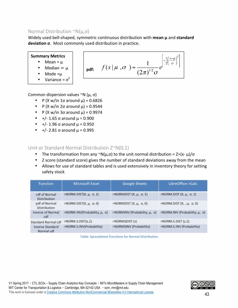
NormalDistribution~N(μ,σ)Widelyusedbell-shaped,symmetriccontinuousdistributionwithmeanμandstandarddeviationσ.Mostcommonlyuseddistributioninpractice.
Commondispersionvalues~N(μ,σ)
• P(Xw/in1σaroundμ)=0.6826• P(Xw/in2σaroundμ)=0.9544• P(Xw/in3σaroundμ)=0.9974• +/-1.65σaroundμ=0.900• +/-1.96σaroundμ=0.950• +/-2.81σaroundμ=0.995
UnitorStandardNormalDistributionZ~N(0,1)• Thetransformationfromany~N(μ,σ)totheunitnormaldistribution=Z=(x-μ)/σ• Zscore(standardscore)givesthenumberofstandarddeviationsawayfromthemean• Allowsforuseofstandardtablesandisusedextensivelyininventorytheoryforsetting
safetystock
Table:SpreadsheetFunctionsforNormalDistribution
SummaryMetrics• Mean=μ• Median= μ• Mode=μ• Variance=σ2
pdf:
Page 44
V1 Spring 2017・CTL.SC0x – Supply Chain Analytics Key Concepts・MITx MicroMasters in Supply Chain Management MIT Center for Transportation & Logistics・Cambridge, MA 02142 USA ・[email protected] This work is licensed under a Creative Commons Attribution-NonCommercial-ShareAlike 4.0 International License. 44
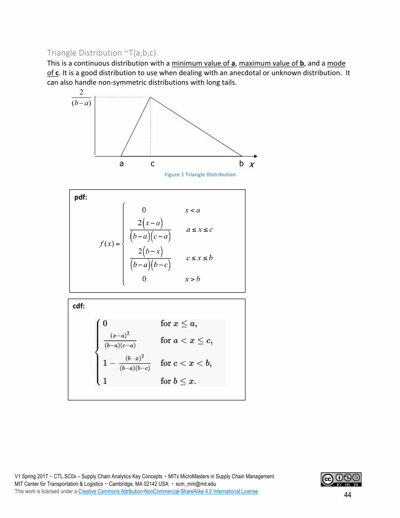
TriangleDistribution~T(a,b,c)Thisisacontinuousdistributionwithaminimumvalueofa,maximumvalueofb,andamodeofc.Itisagooddistributiontousewhendealingwithananecdotalorunknowndistribution.Itcanalsohandlenon-symmetricdistributionswithlongtails.
Figure1TriangleDistribution
Triangle DistributionWe would say,
“X follows a triangle distribution with a minimum of a, maximum b, and a mode of c, ~T(a, b, c)”
22
f (x) =
0 x < a
2 x - a( )b- a( ) c- a( )
a £ x £ c
2 b- x( )b- a( ) b- c( )
c £ x £ b
0 x > b
ì
í
ïïïï
î
ïïïï
a bc
2(b- a)
x
E xéë ùû=a+b+ c
3
Var xéë ùû=118
æ
èç
ö
ø÷ a2 +b2 + c2 - ab-ac-bc( )
P x > déë ùû=b- d( )2
b- a( ) b- c( )
æ
è
ççç
ö
ø
÷÷÷
for c £ d £ b
d = b- P x > déë ùû b- a( ) b- c( ) for c £ d £ b
Characteristics• Good way to get a sense of an unknown distribution• People tend to recall extreme and common values• Handles asymmetric distributions
pdf:
cdf:
Page 45
V1 Spring 2017・CTL.SC0x – Supply Chain Analytics Key Concepts・MITx MicroMasters in Supply Chain Management MIT Center for Transportation & Logistics・Cambridge, MA 02142 USA ・[email protected] This work is licensed under a Creative Commons Attribution-NonCommercial-ShareAlike 4.0 International License. 45
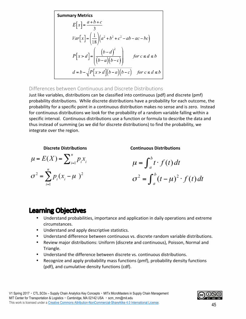
DifferencesbetweenContinuousandDiscreteDistributionsJustlikevariables,distributionscanbeclassifiedintocontinuous(pdf)anddiscrete(pmf)probabilitydistributions.Whilediscretedistributionshaveaprobabilityforeachoutcome,theprobabilityforaspecificpointinacontinuousdistributionmakesnosenseandiszero.Insteadforcontinuousdistributionswelookfortheprobabilityofarandomvariablefallingwithinaspecificinterval.Continuousdistributionsuseafunctionorformulatodescribethedataandthusinsteadofsumming(aswedidfordiscretedistributions)tofindtheprobability,weintegrateovertheregion.
DiscreteDistributions ContinuousDistributions
LearningObjectives• Understandprobabilities,importanceandapplicationindailyoperationsandextreme
circumstances.• Understandandapplydescriptivestatistics.• Understanddifferencebetweencontinuousvs.discreterandomvariabledistributions.• Reviewmajordistributions:Uniform(discreteandcontinuous),Poisson,Normaland
Triangle.• Understandthedifferencebetweendiscretevs.continuousdistributions.• Recognizeandapplyprobabilitymassfunctions(pmf),probabilitydensityfunctions
(pdf),andcumulativedensityfunctions(cdf).
SummaryMetrics
Page 46
V1 Spring 2017・CTL.SC0x – Supply Chain Analytics Key Concepts・MITx MicroMasters in Supply Chain Management MIT Center for Transportation & Logistics・Cambridge, MA 02142 USA ・[email protected] This work is licensed under a Creative Commons Attribution-NonCommercial-ShareAlike 4.0 International License. 46
Page 47
V1 Spring 2017・CTL.SC0x – Supply Chain Analytics Key Concepts・MITx MicroMasters in Supply Chain Management MIT Center for Transportation & Logistics・Cambridge, MA 02142 USA ・[email protected] This work is licensed under a Creative Commons Attribution-NonCommercial-ShareAlike 4.0 International License. 47
Regression
SummaryInthisreviewweexpandourtoolsetofpredictivemodelstoincludeordinaryleastsquaresregression.Thisequipsuswiththetoolstobuild,runandinterpretaregressionmodel.Wearefirstintroducedwithhowtoworkwithmultiplevariablesandtheirinteraction.Thisincludescorrelationandcovariance,whichmeasureshowtwovariableschangetogether.Aswereviewhowtoworkwithmultiplevariables,itisimportanttokeepinmindthatthedatasetssupplychainmanagerswilldealwitharelargelysamples,notapopulation.Thismeansthatthesubsetofdatamustberepresentativeofthepopulation.Thelaterpartofthelessonintroduceshypothesistesting,whichallowsustoanswerinferencesaboutthedata.Wethentacklelinearregression.Regressionisaveryimportantpracticeforsupplychainprofessionalsbecauseitallowsustotakemultiplerandomvariablesandfindrelationshipsbetweenthem.Insomeways,regressionbecomesmoreofanartthanascience.Therearefourmainstepstoregression:choosingwithindependentvariablestoinclude,collectingdata,runningtheregression,andanalyzingtheoutput(themostimportantstep).
KeyConcepts
MultipleRandomVariablesMostsituationsinpracticeinvolvetheuseandinteractionofmultiplerandomvariablesorsomecombinationofrandomvariables.WeneedtobeabletomeasuretherelationshipbetweentheseRVsaswellasunderstandhowtheyinteract.
CovarianceandCorrelationCovarianceandcorrelationmeasureacertainkindofdependencebetweenvariables.Ifrandomvariablesarepositivelycorrelated,higherthanaveragevaluesofXarelikelytooccurwithhigherthanaveragevaluesofY.Fornegativelycorrelatedrandomvariables,higherthanaveragevaluesarelikelytooccurwithlowerthanaveragevaluesofY.Itisimportanttorememberastheold,butnecessarysayinggoes:correlationdoesnotequalcausality.Thismeansthatyouarefindingamathematicalrelationship–notacausalone.
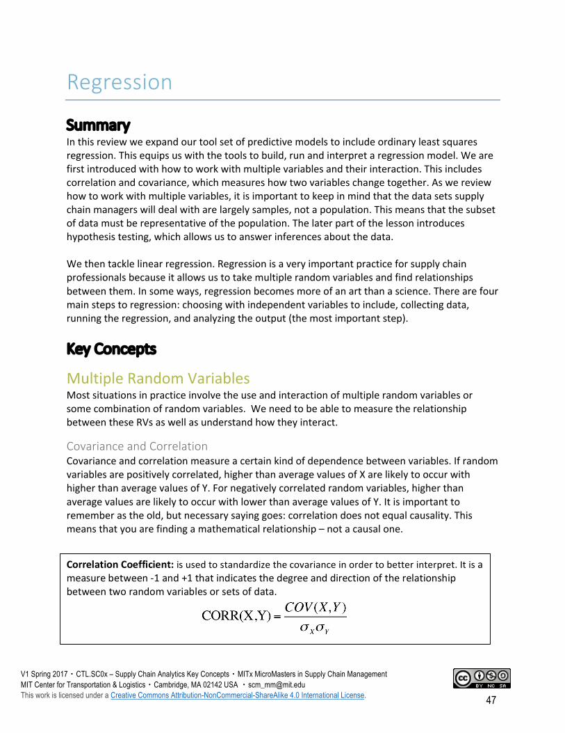
CorrelationCoefficient:isusedtostandardizethecovarianceinordertobetterinterpret.Itisameasurebetween-1and+1thatindicatesthedegreeanddirectionoftherelationshipbetweentworandomvariablesorsetsofdata.
Page 48
V1 Spring 2017・CTL.SC0x – Supply Chain Analytics Key Concepts・MITx MicroMasters in Supply Chain Management MIT Center for Transportation & Logistics・Cambridge, MA 02142 USA ・[email protected] This work is licensed under a Creative Commons Attribution-NonCommercial-ShareAlike 4.0 International License. 48
SpreadsheetFunctionsFunction MicrosoftExcel GoogleSheets LibreOffice->Calc
Covariance =COVAR(array,array) =COVAR(array,array) =COVAR(array;array)
Correlation =CORREL(array,array) =CORREL(array,array) =CORREL(array;array)
LinearFunctionofRandomVariablesAlinearrelationshipexistsbetweenXandYwhenaone-unitchangeinXcausesYtochangebyafixedamount,regardlessofhowlargeorsmallXis.Formally,thisis:Y=aX+b.ThesummarystatisticsofalinearfunctionofaRandomVariableare:
SumsofRandomVariablesIFXandYareindependentrandomvariableswhereW=aX+bY,thenthesummarystatisticsare:
TheserelationsholdforanydistributionofXandY.However,ifXandYare~N,thenWis~Naswell!
CentralLimitTheoremCentrallimittheoremstatesthatthesampledistributionofthemeanofanyindependentrandomvariablewillbenormalornearlynormal,ifthesamplesizeislargeenough.Largeenoughisbasedonafewfactors–oneisaccuracy(moresamplepointswillberequired)aswellastheshapeoftheunderlyingpopulation.Manystatisticianssuggestthat30,sometimes40,isconsideredlargeenough.Thisisimportantbecauseisdoesn’tmatterwhatdistributionstherandomvariablefollows.
Covariance
Expectedvalue:E[W]=aμX+bμYVariance:VAR[W] =a2σ2X+b2σ2Y+2abCOV(X,Y)
=a2σ2X+b2σ2Y+2abσXσYCORR(X,Y)StandardDeviation:σW=√VAR[W]
Expectedvalue:E[Y]=μY=aμX+bVariance:VAR[Y]=σ2Y=a2σ2XStandardDeviation:σY=|a|σX
Page 49
V1 Spring 2017・CTL.SC0x – Supply Chain Analytics Key Concepts・MITx MicroMasters in Supply Chain Management MIT Center for Transportation & Logistics・Cambridge, MA 02142 USA ・[email protected] This work is licensed under a Creative Commons Attribution-NonCommercial-ShareAlike 4.0 International License. 49
Canbeinterpretedasfollows:• Xi,..Xnareiidwithmean=µandstandarddeviation=σ
o ThesumofthenrandomvariablesisSn=ΣXio ThemeanofthenrandomvariablesisX�=Sn/n
• Then,ifnis“large”(say>30)o SnisNormallydistributedwithmean=nµandstandarddeviationσ√no X�isNormallydistributedwithmean=µandstandarddeviationσ/√n
InferenceTesting
SamplingWeneedtoknowsomethingaboutthesampletomakeinferencesaboutthepopulation.Theinferenceisaconclusionreachedonthebasisofevidenceandreasoning.Tomakeinferencesweneedtoasktestablequestionssuchasifthedatafitsaspecificdistributionoraretwovariablescorrelated?Tounderstandthesequestionsandmore–weneedtounderstandsamplingofapopulation.Ifsamplingisdonecorrectly,thesamplemeanshouldbeanestimatorofthepopulationmeanaswellascorrespondingparameters.
• Population:istheentiresetofunitsofobservation• Sample:subsetofthepopulation.• Parameter:describesthedistributionofrandomvariable.• RandomSample:isasampleselectedfromthepopulationsothateachitemisequally
likely.
Thingstokeepinmind• Xisarv~?(µ,σ,...)fortheentirepopulation• X1,X2,...Xnareiid• X�isanestimateofthepopulationparameter,themeanorµ• RememberthatX�isalsoarvbyitself!• x1,x2,...xn,aretherealizationsorobservationsofrvX• xisthesamplestatistic–themean• WewanttofindhowxrelatestoX�relatestoµ
Whydowecare?• WecanshowthatE[X�]=μ andthatS=σ/√n• Note:standarddeviationdecreasesassamplesizegetsbigger!• Also,theCentralLimitTheoremsaysthatsamplemeanX�is~N(μ,σ/√n)
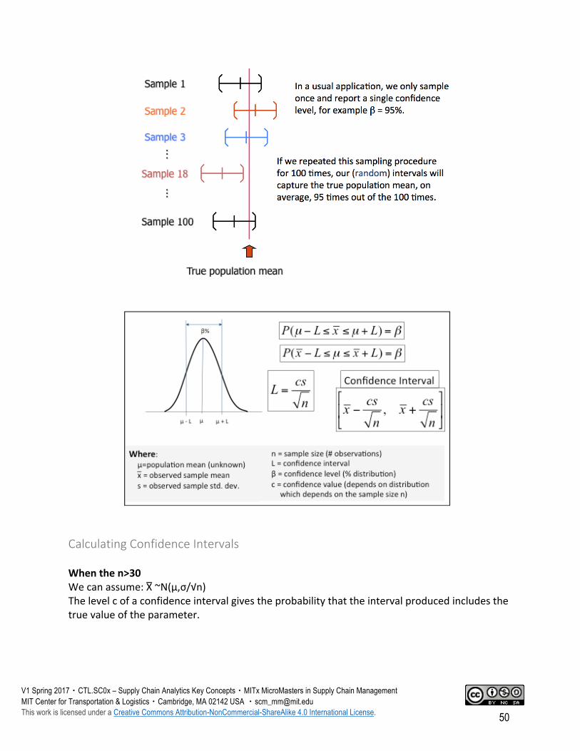
ConfidenceIntervalsConfidenceintervalsareusedtodescribetheuncertaintyassociatedwithasampleestimateofapopulationparameter.
Page 50
V1 Spring 2017・CTL.SC0x – Supply Chain Analytics Key Concepts・MITx MicroMasters in Supply Chain Management MIT Center for Transportation & Logistics・Cambridge, MA 02142 USA ・[email protected] This work is licensed under a Creative Commons Attribution-NonCommercial-ShareAlike 4.0 International License. 50
CalculatingConfidenceIntervalsWhenthen>30Wecanassume:X�~N(μ,σ/√n)Thelevelcofaconfidenceintervalgivestheprobabilitythattheintervalproducedincludesthetruevalueoftheparameter.
Page 51
V1 Spring 2017・CTL.SC0x – Supply Chain Analytics Key Concepts・MITx MicroMasters in Supply Chain Management MIT Center for Transportation & Logistics・Cambridge, MA 02142 USA ・[email protected] This work is licensed under a Creative Commons Attribution-NonCommercial-ShareAlike 4.0 International License. 51
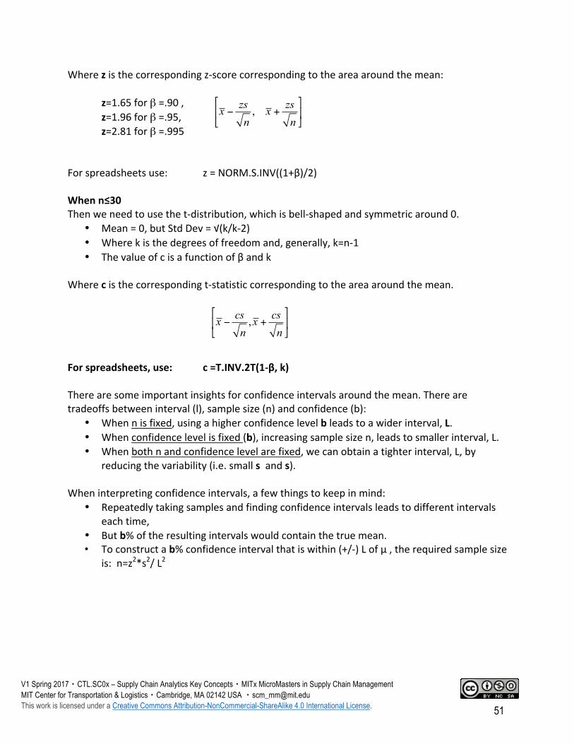
Wherezisthecorrespondingz-scorecorrespondingtotheareaaroundthemean:
z=1.65forβ=.90, z=1.96forβ=.95, z=2.81forβ=.995Forspreadsheetsuse: z=NORM.S.INV((1+β)/2)Whenn≤30Thenweneedtousethet-distribution,whichisbell-shapedandsymmetricaround0.
• Mean=0,butStdDev=√(k/k-2)• Wherekisthedegreesoffreedomand,generally,k=n-1• Thevalueofcisafunctionofβandk
Wherecisthecorrespondingt-statisticcorrespondingtotheareaaroundthemean.Forspreadsheets,use: c=T.INV.2T(1-β,k)Therearesomeimportantinsightsforconfidenceintervalsaroundthemean.Therearetradeoffsbetweeninterval(l),samplesize(n)andconfidence(b):
• Whennisfixed,usingahigherconfidencelevelbleadstoawiderinterval,L.• Whenconfidencelevelisfixed(b),increasingsamplesizen,leadstosmallerinterval,L.• Whenbothnandconfidencelevelarefixed,wecanobtainatighterinterval,L,by
reducingthevariability(i.e.smallsands).
Wheninterpretingconfidenceintervals,afewthingstokeepinmind:• Repeatedlytakingsamplesandfindingconfidenceintervalsleadstodifferentintervals
eachtime,• Butb%oftheresultingintervalswouldcontainthetruemean.• Toconstructab%confidenceintervalthatiswithin(+/-)Lofμ,therequiredsamplesize
is:n=z2*s2/L2
x − zs
n, x + zs
n
⎡
⎣⎢
⎤
⎦⎥
x − cs
n,x + cs
n
⎡
⎣⎢
⎤
⎦⎥
Page 52
V1 Spring 2017・CTL.SC0x – Supply Chain Analytics Key Concepts・MITx MicroMasters in Supply Chain Management MIT Center for Transportation & Logistics・Cambridge, MA 02142 USA ・[email protected] This work is licensed under a Creative Commons Attribution-NonCommercial-ShareAlike 4.0 International License. 52
HypothesisTestingHypothesistestingisamethodformakingachoicebetweentwomutuallyexclusiveandcollectivelyexhaustivealternatives.Inthispractice,wemaketwohypothesesandonlyonecanbetrue.NullHypothesis(H0)andtheAlternativeHypothesis(H1).Wetest,ataspecifiedsignificancelevel,toseeifwecanRejecttheNullhypothesis,orAccepttheNullHypothesis(ormorecorrectly,“donotreject”).TwotypesofMistakesinhypothesistesting:
• TypeI:RejecttheNullhypothesiswheninfactitisTrue(Alpha)• TypeII:AccepttheNullhypothesiswheninfactitisFalse(Beta)• WefocusonTypeIerrorswhensettingsignificancelevel(.05,.01)
Threepossiblehypothesesoroutcomestoatest
• Unknowndistributionisthesameastheknowndistribution(AlwaysH0)• Unknowndistributionis‘higher’thantheknowndistribution• Unknowndistributionis‘lower’thantheknowndistribution
Page 53
V1 Spring 2017・CTL.SC0x – Supply Chain Analytics Key Concepts・MITx MicroMasters in Supply Chain Management MIT Center for Transportation & Logistics・Cambridge, MA 02142 USA ・[email protected] This work is licensed under a Creative Commons Attribution-NonCommercial-ShareAlike 4.0 International License. 53
ExampleofHypothesisTestingIamtestingwhetheranewinformationsystemhasdecreasedmyordercycletime.Weknowthathistorically,theaveragecycletimeis72.5hours+/-4.2hours.Wesampled60ordersaftertheimplementationandfoundtheaveragetobe71.4hours.Weselectalevelofsignificancetobe5%.
1. Selecttheteststatisticofinterest meancycletimeinhours–useNormaldistribution(z-statistic)2.Determinewhetherthisisaoneortwotailedtest Onetailedtest3.Pickyoursignificancelevelandcriticalvalue alpha=5percent,thereforez=NORM.S.INV(.05)=-1.6448
4. FormulateyourNull&Alternativehypotheses H0:Newcycletimeisnotshorterthantheoldcycletime H1:Newcycletimeisshorterthantheoldcycletime
5. Calculatetheteststatistic z=(Xb-μXb)/σXb=(Xb-μ)/(σ/√n)=(71.4–72.5)/(4.2/√60)=-2.0287
6. Comparetheteststatistictothecriticalvaluez=-2.0287<-1.6448theteststatistic<criticalvalue,therefore,werejectthenull
hypothesisRatherthanjustreportingthatH0wasrejectedata5%significancelevel,wemightwanttoletpeopleknowhowstronglywerejectedit.Thep-valueisthesmallestlevelofalpha(levelofsignificance)suchthatwewouldrejecttheNullhypothesiswithourcurrentsetofdata.Alwaysreportthep-valuep-value=NORM.S.DIST(-2.0287)=.0212ChisquaretestChiSquaretestcanbeusedtomeasurethegoodnessoffitanddeterminewhetherthedataisdistributednormally.Touseachisquaretest,youtypicallywillcreateabucketofcategories,c,counttheexpectedandobserved(actual)valuesineachcategory,andcalculatethechi-squarestatisticsandfindthep-value.Ifthep=valueislessthanthelevelofsignificant,youwillthenrejectthenullhypothesis.
Page 54
V1 Spring 2017・CTL.SC0x – Supply Chain Analytics Key Concepts・MITx MicroMasters in Supply Chain Management MIT Center for Transportation & Logistics・Cambridge, MA 02142 USA ・[email protected] This work is licensed under a Creative Commons Attribution-NonCommercial-ShareAlike 4.0 International License. 54
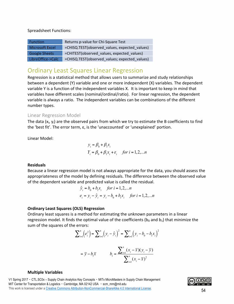
SpreadsheetFunctions:Function Returnsp-valueforChi-SquareTestMicrosoftExcel =CHISQ.TEST(observed_values,expected_values)GoogleSheets =CHITEST(observed_values,expected_values)LibreOffice->Calc =CHISQ.TEST(observed_values;expected_values)
OrdinaryLeastSquaresLinearRegressionRegressionisastatisticalmethodthatallowsuserstosummarizeandstudyrelationshipsbetweenadependent(Y)variableandoneormoreindependent(X)variables.ThedependentvariableYisafunctionoftheindependentvariablesX.Itisimportanttokeepinmindthatvariableshavedifferentscales(nominal/ordinal/ratio).Forlinearregression,thedependentvariableisalwaysaratio.Theindependentvariablescanbecombinationsofthedifferentnumbertypes.
LinearRegressionModelThedata(xi,yi)aretheobservedpairsfromwhichwetrytoestimatetheΒcoefficientstofindthe‘bestfit’.Theerrorterm,ε,isthe‘unaccounted’or‘unexplained’portion.LinearModel:
ResidualsBecausealinearregressionmodelisnotalwaysappropriateforthedata,youshouldassesstheappropriatenessofthemodelbydefiningresiduals.Thedifferencebetweentheobservedvalueofthedependentvariableandpredictedvalueiscalledtheresidual.
OrdinaryLeastSquares(OLS)RegressionOrdinaryleastsquaresisamethodforestimatingtheunknownparametersinalinearregressionmodel.Itfindstheoptimalvalueofthecoefficients(b0andb1)thatminimizethesumofthesquaresoftheerrors:
MultipleVariables
yi = β0 +β1xiYi = β0 +β1xi +εi for i =1,2,...n
yi = b0 +b1xi for i =1,2,...nei = yi − yi = yi −b0 +b1xi for i =1,2,...n
ei2( )i=1
n∑ = yi − yi( )
2
i=1
n∑ = yi −b0 −b1xi( )
2
i=1
n∑
= y −b1x b1 =(xi − x )(yi − y)i=1
n∑
(xi − x )2
i=1
n∑
Page 55
V1 Spring 2017・CTL.SC0x – Supply Chain Analytics Key Concepts・MITx MicroMasters in Supply Chain Management MIT Center for Transportation & Logistics・Cambridge, MA 02142 USA ・[email protected] This work is licensed under a Creative Commons Attribution-NonCommercial-ShareAlike 4.0 International License. 55
Theserelationshipstranslatealsotomultiplevariables.
ValidatingaModelAllstatisticalsoftwarepackageswillprovidestatisticsforevaluation(namesandformatwillvarybypackage).Butthemodeloutputtypicallyincludes:modelstatistics(regressionstatisticsorsummaryoffit),analysisofvariance(ANOVA),andparameterstatistics(coefficientstatistics).OverallFitOverallfit=howmuchvariationinthedependentvariable(y),canweexplain?TotalvariationofCPL–findthedispersionaroundthemean.
Yi = β0 +β1x1i + ...+βk xki +εi for i =1,2,...nE(Y | x1,x2 ,...,xk ) = β0 +β1x1 +β2x2 + ...+βk xkStdDev(Y | x1,x2 ,...,xk ) =σ
ei2( )i=1
n∑ = yi − yi( )
2
i=1
n∑ = yi −b0 −b1x1i − ...−bk xki( )
2
i=1
n∑
TotalSumofSquares
Page 56
V1 Spring 2017・CTL.SC0x – Supply Chain Analytics Key Concepts・MITx MicroMasters in Supply Chain Management MIT Center for Transportation & Logistics・Cambridge, MA 02142 USA ・[email protected] This work is licensed under a Creative Commons Attribution-NonCommercial-ShareAlike 4.0 International License. 56
MakeestimateforofYforeachx.
Modelexplains%oftotalvariationofthedependentvariables.
AdjustedR2correctsforadditionalvariables
IndividualCoefficientsEachIndependentvariable(andb0)willhave:
• Anestimateofcoefficient(b1),• Astandarderror(sbi)
o se=Standarderrorofthemodel
o sx=Standarddeviationoftheindependentvariables=numberofobservations
• Thet-statistic
o k=numberofindependentvariableso bi=estimateorcoefficientofindependent
variable
ErrororResidualSumofSquares
CoefficientofDeterminationorGoodnessofFit(R2)
Page 57
V1 Spring 2017・CTL.SC0x – Supply Chain Analytics Key Concepts・MITx MicroMasters in Supply Chain Management MIT Center for Transportation & Logistics・Cambridge, MA 02142 USA ・[email protected] This work is licensed under a Creative Commons Attribution-NonCommercial-ShareAlike 4.0 International License. 57
Correspondingp-value–TestingtheSlopeo Wewanttoseeifthereisalinearrelationship,i.e.wewanttoseeiftheslope
(b1)issomethingotherthanzero.So:H0:b1=0andH1b1≠0
o Confidenceintervals–estimateanintervalfortheslopeparameter.
Multi-Collinearity,AutocorrelationandHeterscedasticityMulti-Collinearityiswhentwoormorevariablesinamultipleregressionmodelarehighlycorrelated.ThemodelmighthaveahighR2buttheexplanatoryvariablesmightfailthet-test.Itcanalsoresultinstrangeresultsforcorrelatedvariables.Autocorrelationisacharacteristicsofdatainwhichthecorrelationbetweenthevaluesofthesamevariablesisbasedonrelatedobjects.Itistypicallyatimeseriesissue.Heterscedasticityiswhenthevariabilityofavariableisunequalacrosstherangeofvaluesofasecondvariablethatpredictsit.Sometelltalesignsinclude:observationsaresupposedtohavethesamevariance.Examinescatterplotsandlookfor“fan-shaped”distributions.
LearningObjectives
• Understandhowtoworkwithmultiplevariables.• Beawareofdatalimitationswithsizeandrepresentationofpopulation.• Identifyhowtotestahypothesis.• Reviewandapplythestepsinthepracticeofregression.• Beabletoanalyzeregressionandrecognizeissues.
Page 58
V1 Spring 2017・CTL.SC0x – Supply Chain Analytics Key Concepts・MITx MicroMasters in Supply Chain Management MIT Center for Transportation & Logistics・Cambridge, MA 02142 USA ・[email protected] This work is licensed under a Creative Commons Attribution-NonCommercial-ShareAlike 4.0 International License. 58
Simulation
SummaryThisreviewprovidesanoverviewofsimulation.Afterareviewofdeterministic,prescriptivemodeling(optimization,mathprogramming)andpredictivemodels(regression),simulationoffersanapproachfordescriptivemodeling.Simulationsletyouexperimentwithdifferentdecisionsandseetheiroutcomes.Supplychainmanagerstypicallyusesimulationstoassessthelikelihoodofoutcomesthatmayfollowfromdifferentactions.Thisreviewoutlinesthestepsinsimulationfromdefiningthevariables,creatingthemodel,runningthemodel,andrefiningthemodel.Itoffersinsightintothebenefitofusingsimulationforopenendedquestionsbutwarnsofitsexpensiveandtimeconsumingnature. Overthedurationofthecoursewehavereviewedseveraltypesofmodelsincludingoptimization,regression,andsimulation.Optimization(LP,IP,MILP,NLP)isaprescriptiveformofmodelthatfindsthe“bestsolution”and/orprovidesarecommendation.Regressionisapredictiveformofmodelthatmeasurestheimpactofindependentvariablesondependentvariables.Wenowcoversimulation,whichcapturestheoutcomesofdifferentpolicieswithanuncertainorstochasticenvironment.
SimulationSimulationcanbeusedinavarietyofcontexts;itismostusefulincapturingcomplexsysteminteractions,modelingsystemuncertainty,orgeneratingdatatoanalyze,describeandvisualizeinteractions,outcomes,andsensitivities.Thereareseveralclassesofsimulationmodelsincluding:systemdynamics;MonteCarloSimulation;discretetimesimulation;andagentbasedsimulations.Therearefivemainstepsindevelopingasimulationstudy.Formulateandplanthestudy;collectdataanddefineamodel;constructmodelandvalidate;makeexperimentalruns;andanalyzeoutput.Thefollowingwillreviewhoweachofthosestepscanbeconducted.
StepsinaSimulationStudyFormulate&planthestudyOnceithasbeendeterminedthatsimulationistheappropriatetoolfortheproblemunderinvestigation,thenextstepistoformulatetheplanandstudy.Thisinvolvesafewmainsteps:
• Definethegoalsofthestudyanddeterminewhatneedstobesolved• Developamodelwheredailydemandvaries,a“productionpolicy”willbeapplied• Basedondemandandpolicy–calculateprofitability• Assessprofitabilityandperformancemetricsofdifferentpolicies
Collectdata&defineamodel
Page 59
V1 Spring 2017・CTL.SC0x – Supply Chain Analytics Key Concepts・MITx MicroMasters in Supply Chain Management MIT Center for Transportation & Logistics・Cambridge, MA 02142 USA ・[email protected] This work is licensed under a Creative Commons Attribution-NonCommercial-ShareAlike 4.0 International License. 59
Oncetheplanhasbeenformulated,thedataneedstobecollectedandamodeldefined.Ifyouarefacedwithalackofsampledata–youwillneedtodeterminethe“range”ofthevariable(s)bytalkingtostakeholdersorexpertstoidentifypossiblevalues.SomedatacanbederivedfromknowndistributionssuchasPoissonorUniform/TriangularDistributionswhenlittletonoinformationisavailable.Ifsampledataisavailable,conductstepsaswehavepreviouslyreviewedsuchashistograms,calculatingsummarystatistics.ThenconductaChi-Squaretesttofitthesampleto“traditional”distributions.Orusea“custom”empiricaldistributionsuchasdiscreteempirical(use%ofobservationasprobabilities),orcontinuous–usehistogramtocomputeprobabilitiesofeachrangeandthen“uniform”withintherange.InExcel:
=CHITEST(Observed_Range,Actual_Range)–returnsp-value=1-CHIDIST(Chi-square,Degreesoffreedom)–returnsthep-value
Nextstepsareto:
• Determinerelationshipbetweenvariousvariables• Determineperformancemetrics• Collectdata&estimateprobability
Constructmodel&validateMakenecessaryinputsrandom,addadatatabletoautomaterunsofmodel,addsummarystatisticsbasedonresultsfromdatatable.Generatingrandomvariableswiththeunderlyingprincipleofgeneratingarandom(orpseudo-random)numberandtransformittofitthedesireddistribution:
• ManualTechniques:rollingdie,turningaroulettewheel,randomnumbertables• Excel
o RAND()=continuousvariablebetween0and1§ Generaterandomnumberu§ Foreachrandomu,calculateavalueywhosecumulativedistribution
functionisequaltou;assignvalueyasthegeneratednumber:F(y)=P(y)=u
• UniformDistribution~U(a,b)o ~U(a,b)=a+(b–a)*RAND()
• NormalDistribution~N(μ,σ)o ~N(μ,σ)=NORMINV(RAND(),μ,σ)
Chi-SquareTest
Page 60
V1 Spring 2017・CTL.SC0x – Supply Chain Analytics Key Concepts・MITx MicroMasters in Supply Chain Management MIT Center for Transportation & Logistics・Cambridge, MA 02142 USA ・[email protected] This work is licensed under a Creative Commons Attribution-NonCommercial-ShareAlike 4.0 International License. 60
ValidationofModel–istheprocessofdeterminingthedegreetowhichamodelanditsassociateddataareanaccuraterepresentationoftherealworldfortheintendeduseofthemodel.Differentwaysofvalidatingmodelincludingcomparingtohistoricaldataorgettingexpertinput.Oneprimarymethodisparametervariabilityandsensitivityanalysis:
• Generatestatisticalparameterswithconfidenceintervals• HypothesisTesting(seeWeek6)
MakeexperimentalrunsYouwillneedtomakemultiplerunsforeachpolicy;usehypothesistestingtoevaluatetheresults.Ifspreadsheetscontainarandominput,wecanuseourdatatabletorepeatedlyanalyzethemodel.Anadditionalcolumnforrunscanbemade.
AnalyzeoutputAnalyzingoutputdealswithdrawinginferencesaboutthesystemmodelbasedonthesimulationoutput.Needtoensurethatthemodeloutputhasmaintainedaproperbalancebetweenestablishingmodelvalidationandstatisticalsignificance.Dependingonthesystemexamined,simulationwillpotentiallybeabletoprovidevaluableinsightwiththeoutput.Abilitytodrawinferencesfromresultstomakesystemimprovementswillbediscussedfurtherinfuturecourses.
LearningObjectives• Reviewthestepstodevelopingasimulationmodel• Understandwhentouseasimulation,andwhentonot• Recognizedifferentkindsofsimulationsandwhentoapplythem
Page 61
V1 Spring 2017・CTL.SC0x – Supply Chain Analytics Key Concepts・MITx MicroMasters in Supply Chain Management MIT Center for Transportation & Logistics・Cambridge, MA 02142 USA ・[email protected] This work is licensed under a Creative Commons Attribution-NonCommercial-ShareAlike 4.0 International License. 61
ReferencesAPICSSupplyChainCouncil-http://www.apics.org/sites/apics-supply-chain-council
Chopra,Sunil,andPeterMeindl."Chapter1."SupplyChainManagement:Strategy,Planning,andOperation.5thedition,PearsonPrenticeHall,2013.
CouncilofSupplyChainManagementProfessionals(CSCMP)https://cscmp.org/
HillierandLieberman(2012)IntroductiontoOperationsResearch,McGrawHill.Law&Kelton(2000).SimulationModeling&Analysis,McGrawHill.Taha,H.A.(2010).OperationsResearch.Anintroduction.9thedition.PearsonPrenticeHall.Winston(2003)OperationsResearch:ApplicationsandAlgorithms,CengageLearning.TherearemanydifferentbooksbyWayneWinston-theyareallprettygood.