101
Contaminant Modeling with CTRAN/W An Engineering Methodology July 2012 Edition GEO-SLOPE International Ltd.
| Date post: | 28-Feb-2018 |
| Category: |
Documents |
| Upload: | zahmir-mustang |
| View: | 216 times |
| Download: | 0 times |

7/25/2019 Ctran Modeling
http://slidepdf.com/reader/full/ctran-modeling 1/101
Contaminant Modeling
with CTRAN/W
An Engineering Methodology
July 2012 Edition
GEO-SLOPE International Ltd.
7/25/2019 Ctran Modeling
http://slidepdf.com/reader/full/ctran-modeling 2/101
Copyright © 2004-2012 by GEO-SLOPE International, Ltd.
All rights reserved. No part of this work may be reproduced or transmitted in
any form or by any means, electronic or mechanical, including photocopying,
recording, or by any information storage or retrieval system, without the prior
written permission of GEO-SLOPE International, Ltd.
Trademarks: GEO-SLOPE, GeoStudio, SLOPE/W, SEEP/W, SIGMA/W,
QUAKE/W, CTRAN/W, TEMP/W, AIR/W and VADOSE/W are trademarks or
registered trademarks of GEO-SLOPE International Ltd. in Canada and other
countries. Other trademarks are the property of their respective owners.
GEO-SLOPE International Ltd
1400, 633 – 6th Ave SW
Calgary, Alberta, Canada T2P 2Y5
E-mail: [email protected]
Web: http://www.geo-slope.com

7/25/2019 Ctran Modeling
http://slidepdf.com/reader/full/ctran-modeling 3/101
CTRAN/W Table of Contents
Page i
Table of Contents
1 Introduction ......................................................................................... 1
1.1 Typical applications ............................................................................................................. 1
1.2
Contaminant transport processes ....................................................................................... 1
Transport processes ..................................................................................................... 1
Attenuation processes .................................................................................................. 5
1.3 Advective contaminant transport ......................................................................................... 7
1.4 Advective-dispersive contaminant transport ....................................................................... 7
1.5 Density-dependent contaminant transport .......................................................................... 8
1.6 About this book ................................................................................................................... 9
2 Material Properties ............................................................................ 11
2.1
Dispersivity and diffusion .................................................................................................. 11
Diffusion function ........................................................................................................ 11
2.2 Adsorption function ........................................................................................................... 12
Dry density .................................................................................................................. 13
2.3 Decay half life .................................................................................................................... 13
3 Boundary Conditions ........................................................................ 15
3.1 Introduction ....................................................................................................................... 15
3.2 Fundamentals ................................................................................................................... 15
3.3 Boundary condition locations ............................................................................................ 17
Region face boundary conditions ............................................................................... 18
3.4 Sources and sinks ............................................................................................................. 18
3.5 Advection and dispersion considerations ......................................................................... 19
3.6 Source concentration ........................................................................................................ 19
3.7 Surface mass accumulation .............................................................................................. 20
3.8 Exit review ......................................................................................................................... 21
3.9 Concentration vs. mass function ....................................................................................... 23
3.10 Boundary functions ........................................................................................................... 24
3.11
Time activated boundary conditions ................................................................................. 24
3.12 Null elements .................................................................................................................... 24
4
Analysis Types .................................................................................. 25
4.1 Seepage solution interpolation .......................................................................................... 25
4.2 Initial conditions ................................................................................................................. 25
Using an initial conditions file ..................................................................................... 25

7/25/2019 Ctran Modeling
http://slidepdf.com/reader/full/ctran-modeling 4/101
Table of Contents CTRAN/W
Page ii
Activation concentrations............................................................................................ 26
Spatial function for the initial conditions ..................................................................... 26
4.3 Particle tracking analysis .................................................................................................. 26
4.4 Advection-dispersion analysis ........................................................................................... 28
4.5
Density-dependent analysis (with SEEP/W only) ............................................................. 28
4.6 Problem geometry orientation ........................................................................................... 29
Axisymmetric view ...................................................................................................... 29
Plan view .................................................................................................................... 29
2D view ....................................................................................................................... 29
4.7 Staged / multiple analyses ................................................................................................ 30
5
Functions in GeoStudio .................................................................... 33
5.1 Spline functions ................................................................................................................. 33
Slopes of spline functions ........................................................................................... 34
5.2 Linear functions ................................................................................................................. 34
5.3 Step functions ................................................................................................................... 35
5.4 Closed form curve fits for water content functions ............................................................ 36
5.5 Add-in functions ................................................................................................................ 36
5.6 Spatial functions ................................................................................................................ 36
6 Numerical Issues .............................................................................. 39
6.1 Convergence ..................................................................................................................... 39
Vector norms .............................................................................................................. 40
6.2 Numerical dispersion and oscillation ................................................................................. 40
6.3 Peclet and Courant number criteria .................................................................................. 41
6.4 Backward or central difference time integration ................................................................ 42
6.5 Mesh design ...................................................................................................................... 43
6.6 Time step design ............................................................................................................... 43
6.7 Use of the Peclet and Courant numbers criteria ............................................................... 44
6.8 Gauss integration order .................................................................................................... 46
6.9 Equation solvers (direct or parallel direct) ........................................................................ 46
7
Visualization of Results ..................................................................... 49
7.1 Node and element information .......................................................................................... 49
7.2 Particle information ........................................................................................................... 51
7.3 Mass accumulation ........................................................................................................... 52
7.4 Graphing Node and Gauss Data ....................................................................................... 53
7.5 “None” values .................................................................................................................... 56
7/25/2019 Ctran Modeling
http://slidepdf.com/reader/full/ctran-modeling 5/101
CTRAN/W Table of Contents
Page iii
7.6 Projecting Gauss point values to nodes ........................................................................... 57
7.7 Contours ............................................................................................................................ 58
7.8 Water flow vectors and flow paths .................................................................................... 59
7.9 Animation in GeoStudio .................................................................................................... 59
7.10
Flux sections ..................................................................................................................... 59
Flux section theory ..................................................................................................... 59
Flux section application .............................................................................................. 59
7.11 Isolines .............................................................................................................................. 61
8 Modeling Tips and Tricks .................................................................. 63
8.1 Introduction ....................................................................................................................... 63
8.2 Modeling progression ........................................................................................................ 63
8.3 Problem engineering units ................................................................................................ 64
8.4 Fracture flow simulation .................................................................................................... 66
8.5 Flux section location.......................................................................................................... 66
8.6 Unit flux versus total flux? ................................................................................................. 67
9 Illustrative Examples ......................................................................... 69
10 Theory ............................................................................................... 71
10.1 Flow velocity ...................................................................................................................... 71
10.2 Governing equations ......................................................................................................... 71
10.3 Finite element equations ................................................................................................... 76
10.4
Temporal integration ......................................................................................................... 79
10.5 Hydrodynamic dispersion matrix ....................................................................................... 80
10.6 Mass flux ........................................................................................................................... 81
10.7 Dispersive mass flux ......................................................................................................... 82
10.8 Advective mass flux .......................................................................................................... 82
10.9 Stored mass flux ............................................................................................................... 83
10.10 Decayed mass flux ............................................................................................................ 84
10.11 Mass quantity calculation .................................................................................................. 84
10.12 Exit boundaries ................................................................................................................. 85
10.13
Particle tracking ................................................................................................................. 86
10.14 Density-dependent flow .................................................................................................... 87
10.15 Seepage solutions from SEEP/W or VADOSE/W or SIGMA/W ....................................... 88
References ................................................................................................. 89

7/25/2019 Ctran Modeling
http://slidepdf.com/reader/full/ctran-modeling 6/101
Table of Contents CTRAN/W
Page iv

7/25/2019 Ctran Modeling
http://slidepdf.com/reader/full/ctran-modeling 7/101
CTRAN/W Table of Contents
Page v

7/25/2019 Ctran Modeling
http://slidepdf.com/reader/full/ctran-modeling 8/101

7/25/2019 Ctran Modeling
http://slidepdf.com/reader/full/ctran-modeling 9/101
CTRAN/W Chapter 1: Introduction
Page 1
1 Introduction
CTRAN/W is a finite element software product that can be used to model the movement of contaminants
through porous materials such as soil and rock. The comprehensive formulation of CTRAN/W makes it
possible to analyze problems varying from simple particle tracking in response to the movement of water,
to complex processes involving diffusion, dispersion, adsorption, radioactive decay and density
dependencies.
CTRAN/W is integrated with SEEP/W, VADOSE/W and SIGMA/W, other GEO-SLOPE software
products that compute the water flow velocity for a problem. CTRAN/W utilizes the seepage flow
velocities to compute the movement of dissolved constituents in the pore-water. CTRAN/W can only be
used in conjunction with external seepage data. For a density-dependent analysis, CTRAN/W can only be
coupled with SEEP/W. Currently, CTRAN/W does not deal with air phase transport.
1.1 Typic al appl icatio ns
CTRAN/W can be used to model many groundwater contaminant transport problems. This section
presents examples of the types of problems that can be analyzed using CTRAN/W. It should be noted that
CTRAN/W is designed to use the seepage flow velocities computed due to flow in both the saturated and
unsaturated zones. Therefore CTRAN/W is formulated to model saturated/unsaturated contaminant
transport.
The next section provides a review of contaminant transport processes to facilitate the later discussion of
the applications for which CTRAN/W can be used.
1.2 Contaminant transport proc esses
The factors which govern the migration of a contaminant can be considered in terms of transport
processes and attenuation processes. The transport processes can be mathematically represented by
equations based on flow laws. These equations can be combined into a mass balance equation with those
processes causing the attenuation of the contaminant; this yields the general governing differentialequation for contaminant migration.
Transpo r t processes
The two basic transport processes are advection and dispersion. Advection is the movement of the
contaminant with the flowing water. Dispersion is the apparent mixing and spreading of the contaminant
within the flow system. The advection and dispersion transport processes can be illustrated by considering
a steady flow of water in a long pipe filled with sand.
Consider the injection of a slug of contaminant mass into the pipe (Figure 1-1). The mass flows along the pipe with a constant velocity v. This transport process is called advection. As the mass moves along with
the moving water, it also spreads out (i.e., disperses). The contaminant mass occupies an increasinglylonger length of the pipe, thereby decreasing in concentration with time. The spreading out of the
contaminant is called dispersion.
Figure 1-2 illustrates the transport process when a continuous source of contaminant mass is injected into
the pipe. At some point in the pipe beyond the injection location, the contaminant initially appears at a
low concentration and then gradually increases until the full concentration is reached. If only the
advection process is considered, the contaminant would arrive at some point in the pipe as a plug with full

7/25/2019 Ctran Modeling
http://slidepdf.com/reader/full/ctran-modeling 10/101
Chapter 1: Introduction CTRAN/W
Page 2
concentration. Because of dispersion, however, the full concentration arrives at a time later than the first
appearance of the dispersed contaminant, as shown in the figure.
Theoretically, the plug flow arrival time corresponds to the time when the fifty-percent concentrationarrives. The time difference between the first arrival of the dispersed contaminant and the arrival of the
plug flow increases as the distance from the injection point increases.
While the advection process is simply migration in response to the flowing water, the dispersion process
consists of two components. One is an apparent "mixing" and the other is molecular diffusion.
The mixing component, often called mechanical dispersion, arises from velocity variations in the porous
media. Velocity variations may occur at the microscopic level due to the friction between the soil
particles and the fluid and also due to the curvatures in the flow path, as illustrated in Figure 1-3. These
velocity variations result in concentration variations. When the concentration variations are averaged over
a given volume, the contaminant appears to have dispersed.

7/25/2019 Ctran Modeling
http://slidepdf.com/reader/full/ctran-modeling 11/101
CTRAN/W Chapter 1: Introduction
Page 3
Figure 1-1 The Migration and spreading of a contaminant slug in a fluid flowing withvelocity V

7/25/2019 Ctran Modeling
http://slidepdf.com/reader/full/ctran-modeling 12/101
Chapter 1: Introduction CTRAN/W
Page 4
Figure 1-2 Contaminant migration and spreading from a continuous source in a fluidflowing with velocity V

7/25/2019 Ctran Modeling
http://slidepdf.com/reader/full/ctran-modeling 13/101
CTRAN/W Chapter 1: Introduction
Page 5
Figure 1-3 Factors causing mechanical dispersion
Molecular diffusion results in the spreading of contaminant due to concentration gradients. This process
occurs even when the seepage velocity is zero. Molecular diffusion is dependent on the degree of
saturation or volumetric water content of the porous medium, an example of which is shown in Figure
1-4.
In equation form, the dispersion process is characterized as:
* D v Dα = +
where:
D = coefficient of hydrodynamic dispersion,
v = average linear velocity of the flow system,
α = dispersivity of the porous medium, and
D* = coefficient of molecular diffusion.
Attenuat ion processes
Contaminant migration in a porous medium is attenuated by chemical reactions taking place during
transport. These reactions can occur between the contaminant mass and the soil particles or between the
contaminant mass and the pore fluid. Among these reactions, the process of adsorption is believed to be
the most important factor in attenuating the migration of contaminant.
Adsorption causes contaminant mass to be withdrawn from the moving water, reducing the dissolved
concentration and overall rate of contaminant movement. The amount of adsorption that occurs is a
function of the contaminant concentration within the porous medium. This relationship is described by an
adsorption function which relates the adsorption to the concentration. An example of this relationship isshown in Figure 1-5.

7/25/2019 Ctran Modeling
http://slidepdf.com/reader/full/ctran-modeling 14/101
Chapter 1: Introduction CTRAN/W
Page 6
Figure 1-4 Example of molecular diffusion as a function of water content
Figure 1-5 Example of adsorption as a function of concentration
In general, the adsorption characteristic of a contaminant in a soil is represented by a function of S vs. C ,
where S is the mass of contaminant adsorbed per unit mass of soil particles, and C is the concentration of
the contaminant in the porous medium. In the case of a linear function, the slope is called the distribution
coefficient, d K The slope represents the partitioning of the contaminant mass between the solid (soil
particles) and fluid phases of the porous medium. The chemical reactions that cause the partitioning are
assumed to be instantaneous and reversible.
Vol. W. C.
0.0 0.2 0.4 0.6 0.8 1.0
D i f f u s i o n ( l o g 1 0 )
1e-005
0.0001
0.001
Concentration
0.0 0.2 0.4 0.6 0.8 1.0
A d s o r p t i o n
0.0
0.2
0.4
0.6
0.8
1.0
7/25/2019 Ctran Modeling
http://slidepdf.com/reader/full/ctran-modeling 15/101
CTRAN/W Chapter 1: Introduction
Page 7
Another important attenuation process in the case of a radioactive contaminant mass is radioactive decay.
Radioactive decay causes a loss of contaminant mass from the flow system. However, unlike adsorption,
the decayed mass is proportional to the travel time and is irreversible.
1.3 Adv ect ive contam inant transport
As described above, contaminant transport in soils involves the processes of both advection and
dispersion. Early in a contaminant transport analysis, it is often useful to isolate the magnitude of purely
advective transport without the extra data input and computational requirements of including dispersion.
It is impossible to numerically solve the advection-dispersion equation when the dispersive component is
small relative to the advective component, because the numerical solution is unstable in these cases. To
overcome this difficulty, CTRAN/W has an option to simulate the purely advective contaminant transport
process using particle tracking.
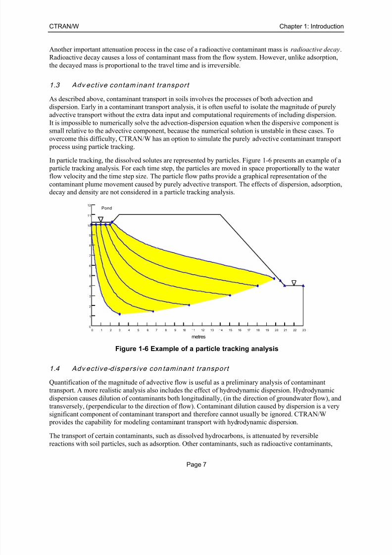
In particle tracking, the dissolved solutes are represented by particles. Figure 1-6 presents an example of a
particle tracking analysis. For each time step, the particles are moved in space proportionally to the water
flow velocity and the time step size. The particle flow paths provide a graphical representation of the
contaminant plume movement caused by purely advective transport. The effects of dispersion, adsorption,
decay and density are not considered in a particle tracking analysis.
Figure 1-6 Example of a particle tracking analysis
1.4 Adv ect ive-dispers ive con taminant transport
Quantification of the magnitude of advective flow is useful as a preliminary analysis of contaminanttransport. A more realistic analysis also includes the effect of hydrodynamic dispersion. Hydrodynamic
dispersion causes dilution of contaminants both longitudinally, (in the direction of groundwater flow), and
transversely, (perpendicular to the direction of flow). Contaminant dilution caused by dispersion is a very
significant component of contaminant transport and therefore cannot usually be ignored. CTRAN/W
provides the capability for modeling contaminant transport with hydrodynamic dispersion.
The transport of certain contaminants, such as dissolved hydrocarbons, is attenuated by reversible
reactions with soil particles, such as adsorption. Other contaminants, such as radioactive contaminants,
Pond
metres
0 1 2 3 4 5 6 7 8 9 10 11 12 13 14 15 16 17 18 19 20 21 22 230
1
2
3
4
5
6
7
8
9
10
11
12
7/25/2019 Ctran Modeling
http://slidepdf.com/reader/full/ctran-modeling 16/101
Chapter 1: Introduction CTRAN/W
Page 8
undergo non-reversible decay reactions that remove them from the groundwater during transport.
CTRAN/W is formulated to include the effects of absorption and decay type reactions during contaminant
transport.
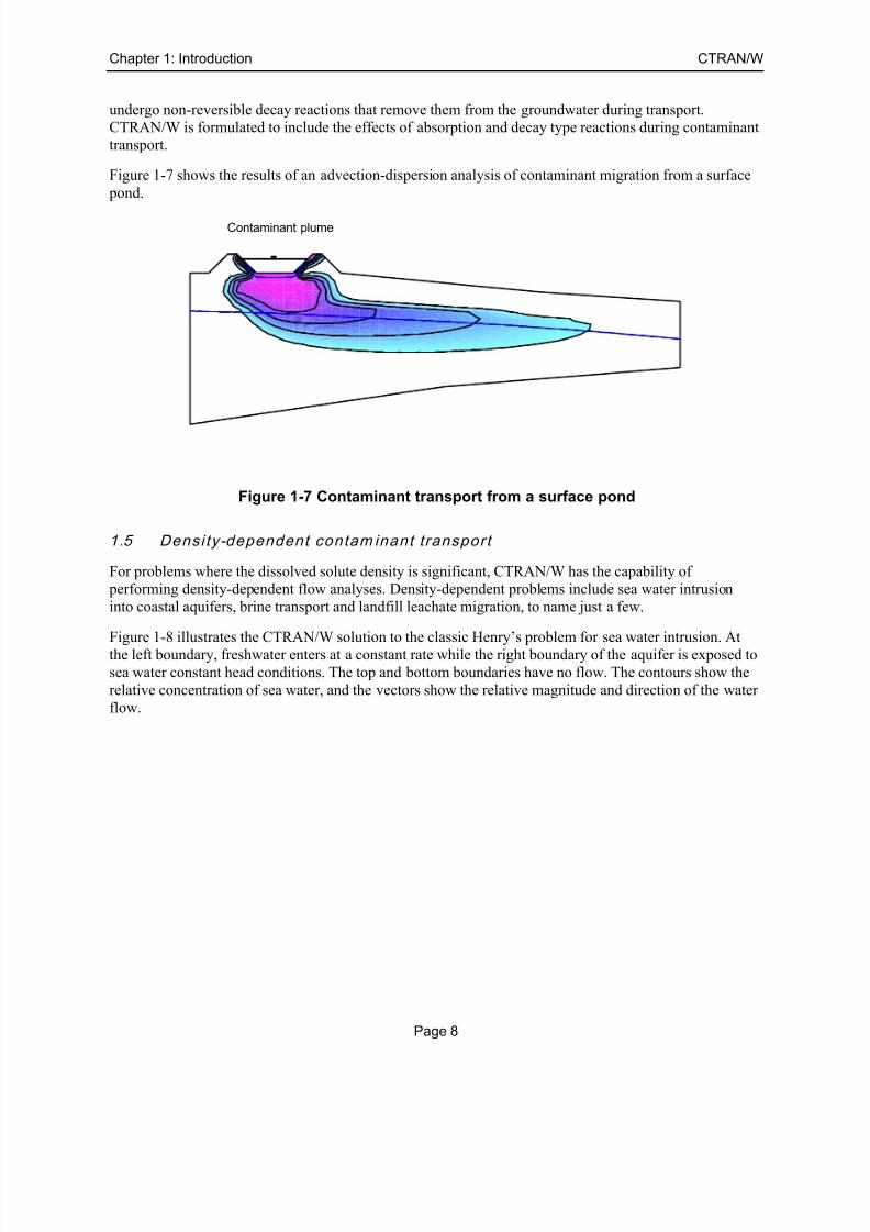
Figure 1-7 shows the results of an advection-dispersion analysis of contaminant migration from a surface
pond.
Figure 1-7 Contaminant transport from a surface pond
1.5 Densi ty-dependent contam inant transport
For problems where the dissolved solute density is significant, CTRAN/W has the capability of
performing density-dependent flow analyses. Density-dependent problems include sea water intrusion
into coastal aquifers, brine transport and landfill leachate migration, to name just a few.
Figure 1-8 illustrates the CTRAN/W solution to the classic Henry’s problem for sea water intrusion. Atthe left boundary, freshwater enters at a constant rate while the right boundary of the aquifer is exposed to
sea water constant head conditions. The top and bottom boundaries have no flow. The contours show the
relative concentration of sea water, and the vectors show the relative magnitude and direction of the water
flow.
Contaminant plume

7/25/2019 Ctran Modeling
http://slidepdf.com/reader/full/ctran-modeling 17/101
CTRAN/W Chapter 1: Introduction
Page 9
Figure 1-8 Sea water intrusion into a coastal aquifer
1.6 About th is book
Modeling the movement of contaminants through soil with a numerical solution can be very complex.
Natural soil deposits are generally highly heterogeneous and non-isotropic. In addition, boundary
conditions often change with time and cannot always be defined with certainty at the beginning of an
analysis. In fact, the correct boundary condition can sometimes be part of the solution as is the case for an
exit review boundary, where the direction of groundwater flow may change between source and sink.
The movement of contaminants can not be modeled without a valid model for groundwater flow in the
system. That is why the MOST important aspect of this type of model is to first be confident in theseepage solution. This book is NOT about seepage modeling and it is assumed from this point onward,
that the reader is familiar with and has read either the SEEP/W or VADOSE/W Engineering Methodology
books. This book is not a stand-alone reference.
While part of this document is about using CTRAN/W to do transport analyses, it is also about general
numerical modeling techniques. Numerical modeling, like most things in life, is a skill that needs to be
acquired. It is nearly impossible to pick up a tool like CTRAN/W and immediately become an effective
modeler. Effective numerical modeling requires some careful thought and planning and it requires a good
understanding of the underlying physical fundamentals. Aspects such as discretization of a finite element
mesh and applying boundary conditions to the problem are not entirely intuitive at first. Time and practice
is required to become comfortable with these aspects of numerical modeling.
Chapter 2 of the SEEP/W and VADOSE/W books is devoted exclusively to discussions on the topic ofHow to Model. The general principles discussed in that book apply to all numerical modeling situations,
even though the discussion there focuses on seepage analysis.
Broadly speaking, there are three main parts to a finite element analysis. The first is discretization –
dividing the domain into small areas called elements. The second part is specifying and assigning material
properties. The third is specifying and applying boundary conditions. Details of discretization are
provided in the SEEP/W or VADOSE/W book, while material properties and boundary conditions as
pertaining to transport analysis are discussed in detail in their respective chapters here.
Freshwater Inflow Sea Water Intrusion
Contours indicate relative concentration of sea water.
0 . 1
0 . 3
0 . 5
0 . 7
0 . 9
Distance (m)
0.0 0.1 0.2 0.3 0.4 0.5 0.6 0.7 0.8 0.9 1.0 1.1 1.2 1.3 1.4 1.5 1.6 1.7 1.8 1.9 2.00.0
0.1
0.2
0.3
0.4
0.5
0.6
0.7
0.8
0.9
1.0
7/25/2019 Ctran Modeling
http://slidepdf.com/reader/full/ctran-modeling 18/101
Chapter 1: Introduction CTRAN/W
Page 10
Transport modeling is numerically challenging because of the presence of a first order transport term in
the main differential equation. For this reason, it is important to have an understanding of how that term
affects the solution of the equation and, in particular, how mesh size and time steps are critical to that
solution. The importance of the Peclet and Courant numbers will be introduced and discussed, along with
other numerical considerations in a chapter titled Numerical Issues.
Two chapters have been dedicated to presenting and discussing illustrative examples. One chapter dealswith examples where geotechnical solutions are obtained by integrating more than one type of analysis,
and the other chapter presents and describes how a series of different geotechnical problems can be
solved.
A full chapter is dedicated to theoretical issues associated with transport and the solution the finite
element equations. Additional finite element numerical details regarding interpolating functions and
infinite elements are given in Appendix A of the SEEP/W and VADOSE/W books.
The chapter entitled “Modeling Tips and Tricks” should be consulted to see if there are simple techniques
that can be used to improve your general modeling method or to help gain confidence and develop adeeper understanding of finite element methods, CTRAN/W conventions or data results.
In general, this book is not a HOW TO USE CTRAN/W manual. This is a book about how to model. It isa book about how to solve transport problems using a powerful calculator; CTRAN/W. Details of how to
use various program commands and features are given in the on line help inside the software.
7/25/2019 Ctran Modeling
http://slidepdf.com/reader/full/ctran-modeling 19/101
CTRAN/W Chapter 2: Material Properties
Page 11
2 Material Properties
This chapter describes the various soil transport properties that are required in the solution of the
CTRAN/W partial differential equation. It is important to have a clear understanding of what the soil
properties mean and what influence they have on the type of results generated. This chapter is not meant
to be an all inclusive discussion of these issues. It is meant to highlight the importance of various parameters and the implications associated with not defining them adequately.
Well defined soil properties can be critical to obtaining an efficient solution of the finite element
equations. When is it acceptable to guess at a function and when must you very carefully define one? Thischapter will address these issues.
2.1 Dispers iv i ty and di f fus ion
For one-dimensional flow, the hydrodynamic dispersion coefficient D is defined above as:
* D v Dα = +
where:
α = dispersivity (material property),
ν = D’Arcy velocity divided by volumetric water content (U /Θ), and
D* = coefficient of molecular diffusion.
Dispersivity is the ratio of the hydrodynamic dispersion coefficient (d) divided by the pore water velocity
(v); thus a = d/v and has units of length. Typically, the dispersivity varies from 0.1 to 100 m however
field and laboratory tests have indicated that dispersivity varies with the scale of the test. Large scale tests
have higher dispersivity than small lab column tests. An approximate value for dispersivity is 0.1 times
the scale of the system (Fetter, 1993). If you are simulating contaminant transport in a 1 m long laboratory
column, then dispersivity ~ 0.1 m. However, if you are simulating transport in a large aquifer greater than1 km in extent, then use dispersivity ~ 100 m.
Dispersion in the direction of the water flow is usually higher than dispersion perpendicular to the flow
direction. Two dispersivity values are therefore required to define the spreading process. Dispersivities in
the flow directions are designated as the longitudinal dispersivity Lα and the transverse dispersivity T
α .
In CTRAN/W if no coefficient of molecular diffusion (D*) is defined, then the dispersion is equal to the
diffusivity in the longitudinal and transverse directions respectively.
Dif fus ion funct ion
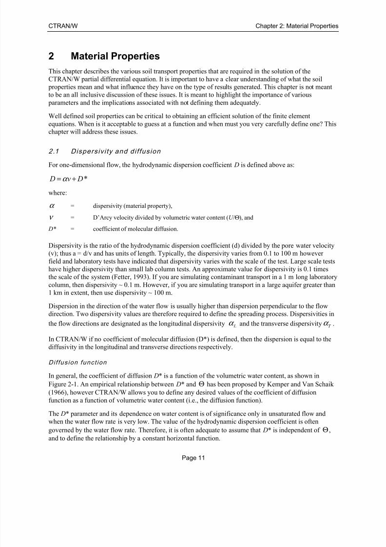
In general, the coefficient of diffusion D* is a function of the volumetric water content, as shown inFigure 2-1. An empirical relationship between D* and Θ has been proposed by Kemper and Van Schaik
(1966), however CTRAN/W allows you to define any desired values of the coefficient of diffusion
function as a function of volumetric water content (i.e., the diffusion function).
The D* parameter and its dependence on water content is of significance only in unsaturated flow and
when the water flow rate is very low. The value of the hydrodynamic dispersion coefficient is often
governed by the water flow rate. Therefore, it is often adequate to assume that D* is independent of Θ ,
and to define the relationship by a constant horizontal function.
7/25/2019 Ctran Modeling
http://slidepdf.com/reader/full/ctran-modeling 20/101
Chapter 2: Material Properties CTRAN/W
Page 12
Figure 2-1 Illustration of a diffusion versus water content function
2.2 Ads orpt ion funct ion
For the transport of a reactive substance, the movement of the mass is also affected by the adsorption of
the solute by the soil particles. As discussed above, the amount of mass adsorbed can be defined in terms
of the mass density of the soil particles. From relationships developed in the Theory chapter, the adsorbed
mass M s is:
s d S ρ =
The rate of change of the adsorbed mass is:
= sd
M S
t t
∂ ∂ ρ
∂ ∂
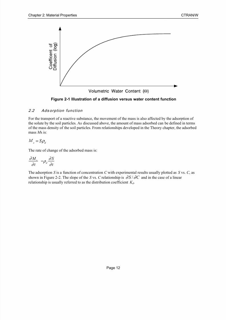
The adsorption S is a function of concentration C with experimental results usually plotted as S vs. C , as
shown in Figure 2-2. The slope of the S vs. C relationship is /S C ∂ ∂ and in the case of a linear
relationship is usually referred to as the distribution coefficient K d .
7/25/2019 Ctran Modeling
http://slidepdf.com/reader/full/ctran-modeling 21/101
CTRAN/W Chapter 2: Material Properties
Page 13
Figure 2-2 Relationship between adsorption and concentration
For many dissolved contaminant and soil combinations, adsorption of contaminant on the soil particles is
linearly related to concentration (e.g. the K d term). CTRAN/W, however, allows a more general relation
to be used to specify the chemical partitioning by allowing the adsorption to be specified as a function of
concentration. The actual slope used in the solution of the equations will be obtained from the function for
any given concentration.
Dry densi ty
The dry density term is the dry mass density of the porous medium. It is multiplied by the adsorption
quantity in the governing equation. The units of dry density are (M/L
3
) must be consistent with the unitsof mass and length.
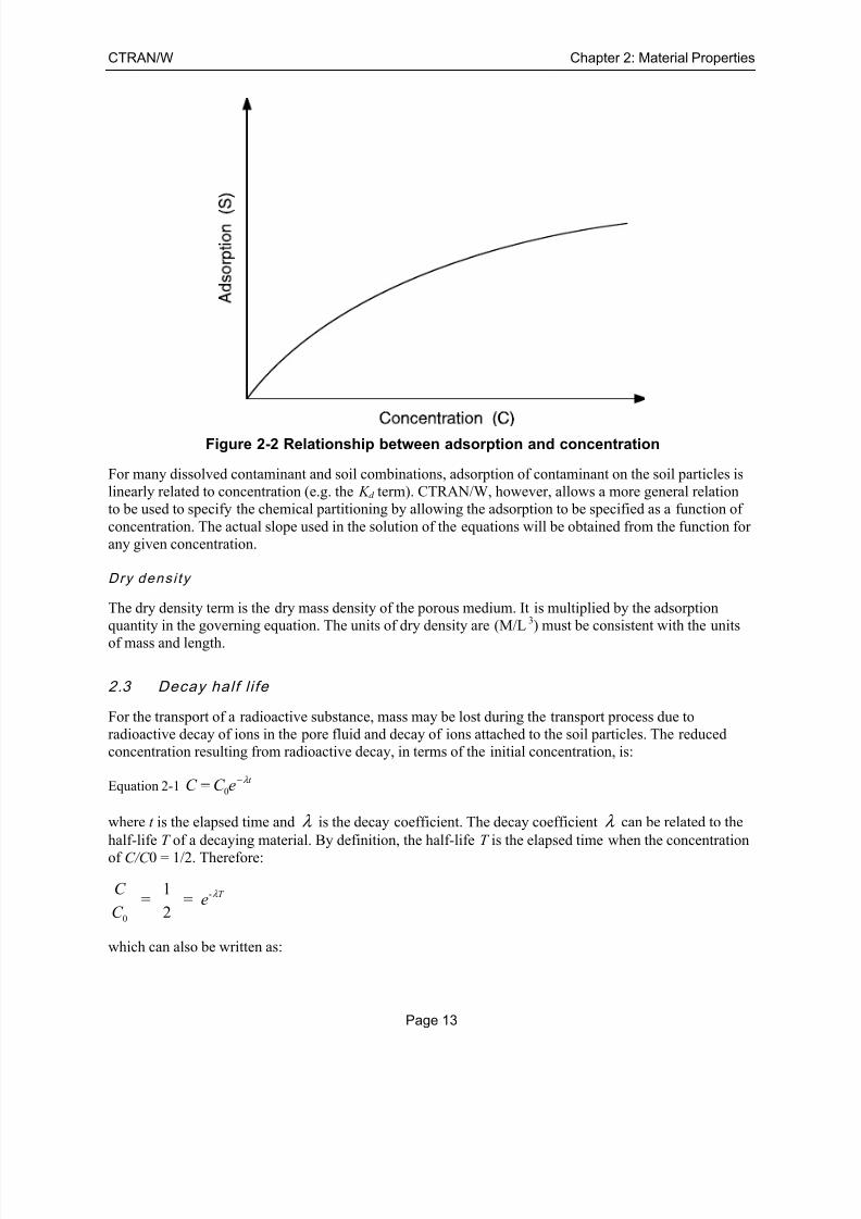
2.3 Decay half l i fe
For the transport of a radioactive substance, mass may be lost during the transport process due to
radioactive decay of ions in the pore fluid and decay of ions attached to the soil particles. The reduced
concentration resulting from radioactive decay, in terms of the initial concentration, is:
Equation 2-1 0
t C C e λ −=
where t is the elapsed time and λ is the decay coefficient. The decay coefficient λ can be related to the
half-life T of a decaying material. By definition, the half-life T is the elapsed time when the concentrationof C/C 0 = 1/2. Therefore:
-
0
1 = =
2
T C e
C
λ
which can also be written as:

7/25/2019 Ctran Modeling
http://slidepdf.com/reader/full/ctran-modeling 22/101
Chapter 2: Material Properties CTRAN/W
Page 14
ln 2 0.693 = =
T T λ
Differentiating Equation 2-1 with respect to time leads to:
= -
C
C t
∂
λ ∂
The amount of radioactive mass in the pore-water M w in an elemental unit volume is C Θ , (see above),
or:
0
t
w C C e λ −= Θ = Θ
The decay half-life must be specified in units of time that are consistent with the units of diffusion. For
example, if the diffusion coefficient is in meters per second (m/sec), then the half-life must be specified in
seconds.
7/25/2019 Ctran Modeling
http://slidepdf.com/reader/full/ctran-modeling 23/101
CTRAN/W Chapter 3: Boundary Conditions
Page 15
3 Boundary Conditions
3.1 Introduct ion
Specifying conditions on the boundaries of a problem is one of the key components of a numerical
analysis. This is why these types of problems are often referred to as “boundary-valued” problems. Beingable to control the conditions on the boundaries is also what makes numerical analyses so powerful.
Solutions to numerical problems are a direct response to the boundary conditions. Without boundary
conditions it is not possible to obtain a solution. The boundary conditions are the driving force. What
causes contaminant to transport? It is the concentration difference between two points or some specified
rate of contaminant flux into or out of the system. The solution is the response inside the problem domain
to the specified conditions on the boundary.
Sometimes specifying conditions is fairly straightforward, such as defining the concentration or
contaminant flux conditions that exist on a year-round basis at the leakage point beneath a waste
collection pond. Many times, however, specifying boundary conditions is complex and requires some
careful thought and planning. Sometimes the correct boundary conditions may even have to be
determined through an iterative process, since the boundary conditions themselves are part of the solution,
as for instance, the contaminant flux from a seepage face where the seepage face is not active continually.
Due to the extreme importance of boundary conditions it is essential to have a thorough understanding of
this aspect of numerical modeling in order to obtain meaningful results. Most importantly, it is essential
to have a clear understanding of the physical significance of the various boundary condition types.
Without a good understanding, it can sometimes be difficult to interpret the analysis results. To assist you
with this aspect of an analysis, CTRAN/W has tools which make it possible verify that the results match
the specified conditions. In other words, do the results reflect the specified or anticipated conditions on
the boundary? Verifying that this is the case is fundamental to confidence in the solution.
This chapter is completely devoted to discussions on boundary conditions. Included are explanations on
some fundamentals, comments on techniques for applying boundary conditions and illustrations of boundary condition types applicable for various conditions.
3.2 Fundamentals
All finite element equations just prior to solving for the unknowns untimely boil down to:
[ ]{ } { } K X A=
where:
[K] = a matrix of coefficients related to geometry and materials properties,
{X} = a vector of unknowns which are often called the field variables, and
{A} = a vector of actions at the nodes.
For a transport analysis the equation is,
Equation 3-1 [ ]{ } { } K C Q=
where:
7/25/2019 Ctran Modeling
http://slidepdf.com/reader/full/ctran-modeling 24/101
Chapter 3: Boundary Conditions CTRAN/W
Page 16
{ }C = a vector of the concentration at the nodes, and
{ }Q = a vector of the contaminant flux quantities at the node.
The prime objective is to solve for the primary unknowns, which in a transport analysis are the
concentrations at each node. The unknowns will be computed relative to the C values specified at somenodes and/or the specified Q values at some other nodes. Without specifying either C or Q at some nodes,
a solution cannot be obtained for the finite element equation. In a steady-state analysis, at least one node
in the entire mesh must have a specified C condition. The specified C or Q values are the boundary
conditions.
A very important point to note here is that boundary conditions can only be one of two options. We can
only specify either the C or the Q at a node. It is very useful to keep this in mind when specifying
boundary condition. You should always ask yourself the question: “What do I know? Is it the C or the
contaminant flux, Q?” Realizing that it can be only one or the other and how these two variables fit into
the basic finite element equation is a useful concept to keep in mind when you specify boundary
conditions.
As we will see later in this chapter, flux across a boundary can also be specified as a gradient or a rate per
unit area. Such specified transport boundary conditions are actually converted into nodal Q values. So,
even when we specify a gradient, the ultimate boundary condition options still are either C or Q.
Remember! When specifying transport boundary conditions, you only have one of two fundamental options – you
can specify C or Q. These are the only options available but they can be applied in various ways.
Another very important concept you need to fully understand is that when you specify C, the solution to
the finite element Equation 3-1 will provide Q. Alternatively, when you specify Q, the solution will
provide C. The equation always needs to be in balance. So when a C is specified at a node, the computed
Q is the Q that is required to maintain the specified C. When Q is specified, the computed C is the C thatis required to maintain the specified flux Q.
Recognizing the relationship between a specified nodal value and the corresponding computed value is
useful when interpreting results. Assume you know the specified flux across a surface boundary. Later
when you check the corresponding computed concentration at that node you may find that it is
unreasonably high or low. You would use your knowledge of the problem to assess if the contaminant
flux applied was reasonable. The C values are computed based on Q and the soil properties, so it must be
one of three things. Knowing what to look for helps you to judge whether that is reasonable or not.
CTRAN/W always provides the corresponding alternative when conditions are specified at a node. When
C is specified, Q is provided, and when Q is specified, C is provided. The computed Q values at nodes
where a concentration is specified are referred to as Boundary Flux values with units of mass of
contaminant per time (e.g. M/t). These Boundary Flux values are listed with all the other information provided at nodes.
A third important fundamental behavior that you need to fully understand is that when neither C nor Q is
specified at a node, the computed Q is zero. Physically, what it means is that the contaminant flux coming
towards a node is the same as the flux leaving the node. Another way to look at this is that no
contaminant is entering or leaving the system at these nodes. Contaminant leaves or enters the system
only at nodes where C or a non-zero Q has been specified. At all nodes for no specified condition, Q is

7/25/2019 Ctran Modeling
http://slidepdf.com/reader/full/ctran-modeling 25/101
CTRAN/W Chapter 3: Boundary Conditions
Page 17
always zero. This, as we will see later in this chapter, has important implications when simulating features
such as point sources of contaminants at a single node.
The concentrations in a transport analysis are the primary unknowns or field variables. A boundarycondition that specifies the field variable (C) at a node is sometimes referred to as a Type One or a
Dirichlet boundary condition. Transport gradient (flux) boundary conditions are often referred to as Type
Two or Neumann boundary conditions. You will encounter these alternate names in the literature but theyare not used here. This document on transport modeling simply refers to boundary conditions as
concentration (C) or contaminant flux (Q) boundary conditions. Later we will differentiate between nodal
flux Q and specified gradients (rates of flux per unit area) across an element edge.
3.3 Bou ndary cond i t ion locat ions
In GeoStudio, all boundary conditions must be applied directly on geometry items such as region faces,
region lines, free lines or free points. There is no way to apply a BC directly on an element edge or node.
The advantage of connecting the BC with the geometry is that it becomes independent of the mesh and
the mesh can be changed if necessary without losing the boundary condition specification. If you keep
the concept of BC’s on geometry in mind, you will find that you can specify any location for a BC quite
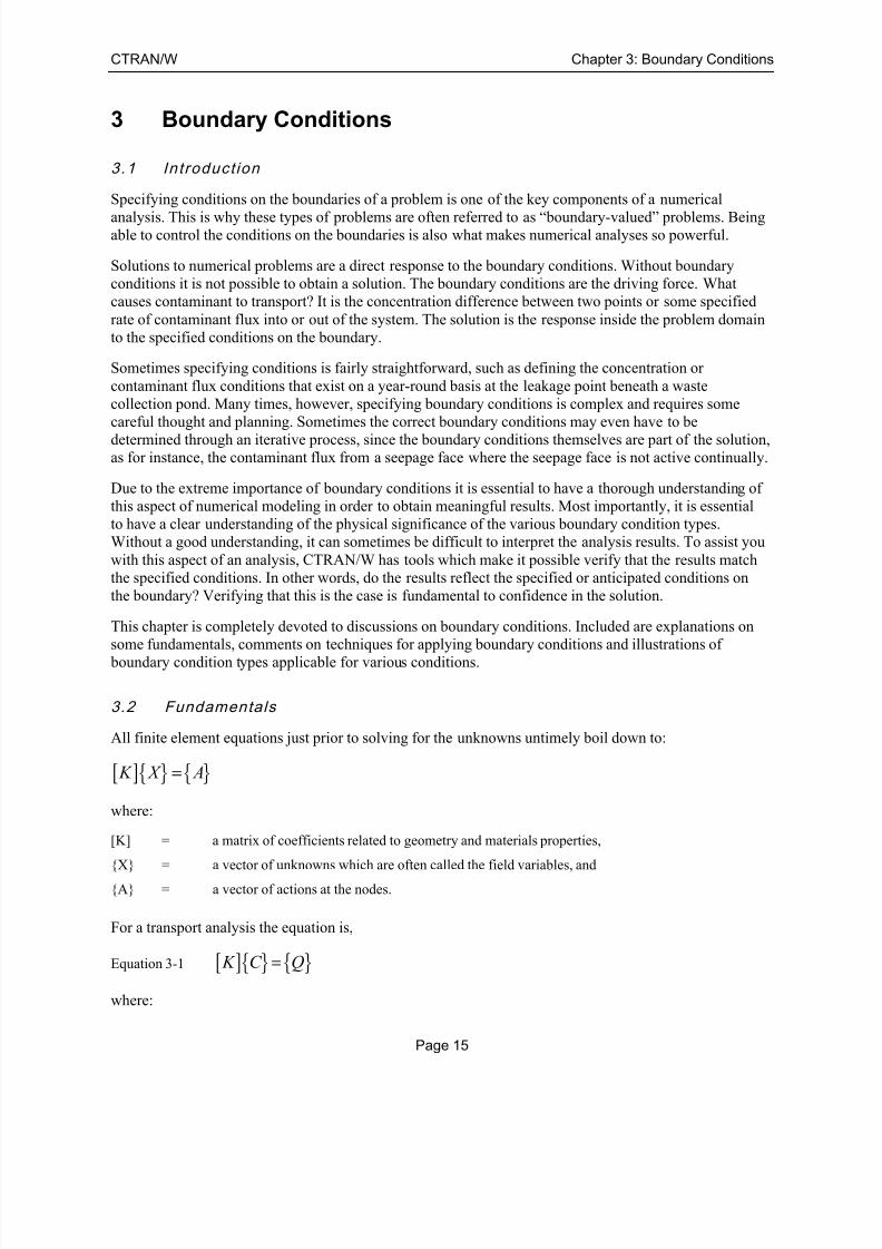
easily. Consider the following examples which show the desired location of boundary conditions, the boundary condition applied to the geometry, and finally the underlying mesh with boundary conditions
visible.
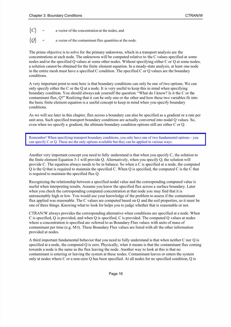
If you look carefully at Figure 3-2 and Figure 3-3 you will see that the BC symbols along the slope edge
are spaced differently. In the view with no mesh visible, the BC’s are displayed at a spacing that depends
on the scale and zoom factor of the page. In the image with the mesh visible, the BC’s are drawn exactly
where they will appear. They are always at a node for this type of BC. Notice also that the free point
location forces a mesh node to be at the exact location. This way, you can always define a BC anywhere
you want and when the mesh changes, the BC location will remain fixed.
Figure 3-1 Desired BC locations
Along a region edge sub-division
At a free point
7/25/2019 Ctran Modeling
http://slidepdf.com/reader/full/ctran-modeling 26/101
Chapter 3: Boundary Conditions CTRAN/W
Page 18
Figure 3-2 BC's attached to geometry
Figure 3-3 BC's with underlying mesh visible
Region face boundary cond i t ions
A flux or stress boundary condition, which is given in units per area, can be applied to the “face” of aregion. GeoStudio uses the contributing area that surrounds each node to calculate the corresponding
flow rate or force. For example, a stress boundary condition applied to a region face is multiplied by the
area that surrounds a node and converted into a force at the nodes. Similarly, a heat flux rate of 1kJ/m2/day would be converted into a flow rate (kJ/day) after integration.
3.4 Sources and sinks
There is another type of boundary condition called a source or a sink. These boundary conditions are
sometimes referred to as a Type 3 boundary condition. A typical sink might represent a drain at some
point inside a mesh where contaminant is added or removed. The important concept about sinks and
sources is that they represent mass flux into or out of the system.
In CTRAN/W flux boundary conditions can be applied along outside edges or nodes of the mesh, or
along inside edges or nodes. There is no difference in how the equations are solved in either case. The
only thing to watch for is that you have an understanding of the area that the contaminant transports
across.
There are a couple special types of boundary conditions that have been formulated directly in CTRAN/W:
the surface mass accumulation condition and the exit review condition. These are discussed in more detail
below.
Along a region edge sub-division
At a free point
Along a region edge sub-division
At a free point

7/25/2019 Ctran Modeling
http://slidepdf.com/reader/full/ctran-modeling 27/101
CTRAN/W Chapter 3: Boundary Conditions
Page 19
3.5 Adv ect ion and dispers ion cons iderat ions
When you specify the boundary conditions in a contaminant transport analysis, it is important to
recognize that there are two processes by which mass is carried across a boundary: one is by advection
and the other is by dispersion. The advective component is due to the water movement across a boundary
while the dispersive process is due to the chemical (concentration) gradients between the boundary nodes
and the nodes immediately inside the boundary.
The advective component of the boundary mass flux is related to the water flux (Qw) across the
boundary. This information is obtained from a SEEP/W analysis. CTRAN/W uses the nodal Qw values
from the SEEP/W file to compute the advective boundary flux.
When specifying boundary conditions for a transport analysis, you will often find it useful to first get a
clear picture of the water flux across the boundaries. A clear understanding of the boundary water flux is
essential in the specification of boundary conditions and the interpretation of computed results.
3.6 Source conc entrat ion
Consider the case illustrated in Figure 3-4 where the leakage from the lagoon is the source of the
contamination. If the concentration of the contaminated fluid in the lagoon is known, you can specify the
boundary condition type as C s (the concentration of the source).
Figure 3-4 Illustration of a lagoon with contaminated fluid
When you specify C s as the boundary condition type, CTRAN/W uses the concentration of the source to
compute a nodal mass flux at the boundary. The mass flux is computed as:
= *mass w sQ Q C
where:
Qmass = nodal total mass flux,
Qw = nodal water flux from SEEP/W, and
Cs = user-specified concentration of the source.
Specifying a C s boundary at the nodes is different than specifying a C boundary with a value equal to C s.
By specifying C s at a boundary, you are actually defining a mass flux type boundary. When specifying C ,
you are defining a specified concentration type boundary.

7/25/2019 Ctran Modeling
http://slidepdf.com/reader/full/ctran-modeling 28/101
Chapter 3: Boundary Conditions CTRAN/W
Page 20
When you specify C s at a node, the computed nodal concentration will be less than C s during the early
stage of the transport process. After some time, the computed concentration will become equal to C s.
However, if you specify a C boundary with a value equal to C s, the computed nodal concentration will be
equal to C s immediately.
In general, using C s as a boundary condition is a more realistic option than simply specifying
concentration at the nodes. In addition, it has the advantage of not creating excessive initial concentrationgradients, as is the case with specified concentration boundaries. The gradual build-up of concentration at
C s nodes tends to reduce numerical difficulties that may arise from excessively high concentration
gradients.
NOTE: Specifying a Cs boundary in a node with zero nodal flux is the same as specifying the node as a
zero mass flux boundary (i.e., Qm = 0.0 or qm = 0.0).
3.7 Surface mass accumulat ion
Slow, contaminated moisture flow to the ground surface (or evaporative water flux) can result in an
accumulation of the solute on the surface boundary. In such cases, the water evaporates, but the solute
remains and accumulates with time, as illustrated in Figure 3-5.
The solute accumulation at the ground surface can be simulated with CTRAN/W by specifying a zero
mass flux at the surface (i.e., Qm = 0.0 or qm = 0.0). A zero mass flux means that no mass gain or loss is
allowed across the boundary. In other words, contaminant mass carried by the water flow to the boundary
is not allowed to leave; consequently, the mass accumulates at the boundary.
Figure 3-5 Illustration of mass accumulation on evaporative ground surface
In technical terms, the advective flux carries the contaminant solute to the boundary. Physically, the water
flux will cause advective mass loss across the boundary; however, because of the specified zero mass flux boundary condition, the boundary develops a reverse dispersive mass flux equal in magnitude but
opposite in direction to the advective mass loss. The reverse dispersive mass flux causes the increase in
concentration.
For the mass to accumulate at the boundary there must be water flux loss across the boundary. There will
be no solute accumulation if there is no water flow across the boundary (i.e., qw = 0.0).
The default boundary condition in CTRAN/W is a no-mass flux condition, (i.e., Qm = 0.0 or qm = 0.0).
Specifying a boundary type as none is the same as specifying Qm or qm equal to zero.

7/25/2019 Ctran Modeling
http://slidepdf.com/reader/full/ctran-modeling 29/101
CTRAN/W Chapter 3: Boundary Conditions
Page 21
3.8 Exit review
At a boundary where neither the mass flux nor the concentration are known, or where the nodal water flux
may reverse in direction during the transport process, you may specify the boundary as an Exit Review
boundary. When a boundary node is specified with Exit Review, the node is checked to see if an exit
boundary should be applied at each time step. If the water flux of the node is negative (i.e., water flux is
exiting at the boundary), the boundary condition of the node will be changed to an exit boundary. If thewater flux of the node is zero or positive, the boundary condition of the node is not changed.
CTRAN/W offers two types of exit boundaries. The first and simplest option is one that ignores the
dispersive flux across the exit boundary (Qd = 0), and is often referred to as a zero dispersive mass flux
exit boundary. With this type of exit boundary, contaminant mass is assumed to leave the exit boundary
by advection only. As a result, the concentration gradients at the boundary are forced to be zero, which
causes the concentration contours to be perpendicular to the exit boundary. The second type of exit
boundary condition accounts for both advective and dispersive mass flux at the boundary (Qd > 0), and is
referred to as a free exit boundary. A free exit boundary accounts for both advective and dispersive mass
flux across the boundary, which generally gives more realistic results. It is best to use the free exit
boundary unless there is a specific reason for using the zero dispersive mass flux exit boundary.
The “Example” problem in the Illustrative Examples chapter illustrates a typical situation where an exit boundary is required. Contaminant mass is existing at the downstream toe of dam. Since neither the mass
flux nor the concentration are known at the boundary, the boundary is specified as Qm =0 conditions with
review for free exit boundary (Qd > 0).
The Exit Review feature is particularly useful in a density-dependent flow problem. Using Henry’s sea
water intrusion problem presented in the Illustrative Examples chapter, sea water may enter the flow
system along the bottom portion of the sea water boundary and freshwater may exit along the upper
portion. Since the interface between the sea water and the freshwater is not known, it is best to specify the
entire vertical boundary as Cs = 1 and review for free exit boundary.
Figure 3-6 is the solution to Henry’s sea water intrusion problem when the right boundary is simulated as
a C boundary condition with no exit review. Figure 3-7 is the solution to the same problem except that theright boundary is specified as a Cs boundary type condition with exit review Qd > 0. In the latter case, the
nodes along the upper portion of right boundary were converted to an exit boundary by the exit review
feature.
Allowing the sea water boundary to be reviewed for free exit boundary conditions provides a more physically realistic solution than when the concentration is specified along the sea water boundary. The
difference between the two solutions is primarily in the concentration distribution along the upper portion
of the sea water boundary. Without exit review, the concentration of the nodes along the upper portion of
the right boundary are equal to your specified value at all times; whereas with exit review, the nodes may
be converted to free exit boundary, and the concentration is solved for at each time step.

7/25/2019 Ctran Modeling
http://slidepdf.com/reader/full/ctran-modeling 30/101
Chapter 3: Boundary Conditions CTRAN/W
Page 22
Figure 3-6 contour of Henry's problem, no exit review
Figure 3-7 Concentration contour of Henry's problem with exit review
Note that Exit Review specification is only allowed for mass flux type boundary conditions, (i.e. Qm, qm
and Cs), where the nodal concentration are computed.
Exit boundaries should only be applied to regions with four-noded quadrilateral elements and must bespecified along only the edge defined by elements with two nodes. When each element matrix equation is
calculated in SOLVE, a surface integral term is formed for element edges that are exit boundaries. This
surface integral cannot be formed for higher order elements; and therefore, application of exit boundaries
to higher ordered elements is invalid.
The exit surface integral can be formed for three-noded triangular elements if two of the three nodes areon an exit boundary. However, using an exit boundary on a triangular element often is of limited value,
since any adjacent triangular elements usually have only one node on the exit boundary. In this case, the
surface integral is formed only for every second triangular element.
In summary, the best exit boundary results are obtained with four-noded quadrilateral elements. Three-
noded triangular elements can be used but do not give the best results and higher-order elements cannot
be used along an exit boundary.
0 . 2
0 . 4
0 . 6
0 . 8
0.0 0.1 0.2 0.3 0.4 0.5 0.6 0.7 0.8 0.9 1.0 1.1 1.2 1.3 1.4 1.5 1.6 1.7 1.8 1.9 2.00.0
0.1
0.2
0.3
0.4
0.5
0.6
0.7
0.8
0.9
1.0
0 . 2
0 . 4
0 . 6
0 . 8
0.0 0.1 0.2 0.3 0.4 0.5 0.6 0.7 0.8 0.9 1.0 1.1 1.2 1.3 1.4 1.5 1.6 1.7 1.8 1.9 2.00.0
0.1
0.2
0.3
0.4
0.5
0.6
0.7
0.8
0.9
1.0

7/25/2019 Ctran Modeling
http://slidepdf.com/reader/full/ctran-modeling 31/101
CTRAN/W Chapter 3: Boundary Conditions
Page 23
3.9 Concentrat ion vs. mass funct ion
A special type of boundary function can be used to simulate, for example, the case where a contaminant
flows into a body of fresh water. Figure 3-8 illustrates this example. Initially, the boundary condition of
the fresh water pond can be specified as a zero concentration boundary, (i.e. C =0). As the contaminant
flows into the pond, the concentration of the water increases with time.
The concentration boundary condition of the pond therefore has to be modified with time. The
concentration of the pond can be computed at any time if you know the accumulated mass discharged into
the pond and the volume of the pond. In equation form, the pond concentration is:
= pond
accumulated massC
pond volume
This relationship can be used to develop a C vs. mass function, (Figure 3-9), which can be specified as a
boundary condition.
When using this boundary type, CTRAN/W computes the accumulated mass that flows into the pond at
the end of each time step. This value, together with the boundary function, is then used to compute the
boundary concentration at the start of a new time step.
Figure 3-8 Illustration of contaminant discharge into a fresh water pond
Figure 3-9 Illustration of a concentration versus mass boundary function
Mass
0 5 10 15
C o n c e n t r a t i o n
10
12
14
16
18
20

7/25/2019 Ctran Modeling
http://slidepdf.com/reader/full/ctran-modeling 32/101
Chapter 3: Boundary Conditions CTRAN/W
Page 24
3.10 Bou ndary funct ion s
CTRAN/W is formulated to accommodate a very wide range of boundary conditions. In a steady state
analysis, all of the boundary conditions are either fixed concentrations or fixed flux values. In a transient
analysis however, the boundary conditions can also be functions of time or in response to transport
amounts exiting or entering the transport regime. CTRAN/W accommodates a series of different
boundary functions. Each one is discussed in this section.
3.11 Time act ivated bou ndary cond i t ions
There are situations where the actual position of a boundary condition may change with time. A typical
case may be the placement of mining tailings. The thickness of the tailings grows with time and yet there
is always some water on the surface. The position of the head equal elevation (zero pressure) changes
with time. Another case may be in the simulation of constructing an embankment in lifts. The hydraulic
boundary condition changes with time. This type of boundary condition is only useful when elements are
activated or deactivated with time for the purpose of simulating fill placement or constructing an
excavation.
Time activated boundary conditions are currently under development for a future version of GeoStudio.
3.12 Null elements
There are many situations where only a portion of the mesh is required. Parts of the mesh that are not
required in a CTRAN/W analysis can be flagged as null elements. Consider a case where you want to use
a similar mesh in different GeoStudio analyses. In the case of a cutoff wall to prevent water flow, you
could set those elements as NULL in the seepage analysis. This would treat the elements as if they were
not a part of the mesh and water would not flow around them. However, if you now wanted to model the
contaminant transport in this scenario, you would turn the elements back on in CTRAN/W and assign
them valid properties.
Elements present but not required in a particular analysis can be assigned a material type (number) thatdoes not have an assigned conductivity function. Elements with this uncharacterized material are treated
as null elements. As far as the main solver is concerned, these elements do not exist.

7/25/2019 Ctran Modeling
http://slidepdf.com/reader/full/ctran-modeling 33/101
CTRAN/W Chapter 4: Analysis Types
Page 25
4 Analysis Types
There are two fundamental types of finite element contaminant transport analysis: advection / dispersion,
or density-dependent. A further option for simple particle tracking is also available. In terms of the
seepage solution used with CTRAN/W, it can be steady state or transient. Full details of steady state and
transient seepage analysis are provided in the SEEP/W or VADOSE/W engineering books. A description
of each type of contaminant analysis and the implications associated with each type are discussed in this
chapter.
4.1 Seepage solu tion interp olat ion
The accuracy of the contaminant transport solution is directly dependent on the accuracy of the seepage
solution. In other words, you must be able to obtain a reasonable seepage solution of a flow system first
before conducting the transport analysis.
CTRAN/W relies on a seepage solution generated by either SEEP/W or VADOSE/W to perform the
contaminant transport analysis. For a steady-state seepage analysis, the seepage solution is assumed to be
constant during the transport process. For a density-dependent analysis, the time steps specified in the
CTRAN/W data file are used to compute the seepage solution in SEEP/W (VADOSE/W does not support
density-dependent analysis). For transient seepage analysis, CTRAN/W interprets the seepage solution as
a step function. For example, if seepage solutions are only available for three elapsed time steps at 100,
200 and 400 minutes, in a transport analysis, the seepage solution is assumed to be constant between 0 to
100 minutes, 100 to 200 minutes and 400 minutes or more.
In situations where the boundary condition is not constant and a more precise seepage solution is
required, you may be required to do one of the following:
• Use smaller time step increments, especially in a period in which changes in boundary
condition are anticipated. The approximation error resulting from the step function decreases
as the time step increments become smaller.
• Use the same time step increments in both the seepage model and CTRAN/W, so that the
exact seepage solution at a certain time is computed rather than interpolated.
4.2 Init ial co ndit io ns
The initial concentration of all nodes must be defined in a transport analysis regardless of whether it is an
advection-dispersion or density-dependent problem. CTRAN/W allows you to specify the initial
conditions by either reading the data from an initial conditions file, or by specifying the initial
concentration as a material property. By default, when initial conditions are not specified, CTRAN/W
assumes the initial concentration of all nodes to be zero. A zero initial concentration condition represents
a clean flow system at the beginning of a transport process.
NOTE: The initial concentration of a node is independent of the boundary condition of the node. In otherwords, a particular node may have an initial concentration of 100 units specified, with a C boundary
condition of 0 units also specified.
Using an in i t ia l condi t ions f i le
With this option, you specify an initial conditions file by choosing the file name in the analysis settings
command dialogue. You can choose a parent file within the same project or an external file.
7/25/2019 Ctran Modeling
http://slidepdf.com/reader/full/ctran-modeling 34/101
Chapter 4: Analysis Types CTRAN/W
Page 26
Act ivat ion concentrat ions
If you have new soil region becoming active and you know it has a certain initial concentration, you can
use the material property activation concentration value to initialize the concentrations in that region.This value is only applied the first time a new region is active in the analysis. This approach can be used
to set initial concentrations at the start of any analysis, not just a construction sequence analysis.
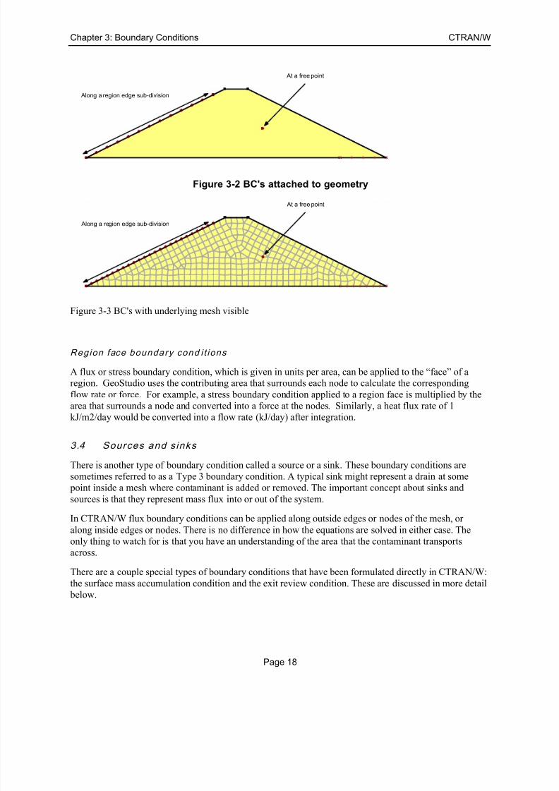
Spat ia l funct ion for the in i t ial cond i t ions
A third option is to specify directly what you think the starting concentrations conditions will be by
applying a spatial function. You can define a spatial function for concentrations and have the solver
point to this function result. An example of a spatial function is shown below. Most of the functionsdata points indicate a concentration of zero with a small contaminated zone at the base of the slope.
Figure 4-1 Spatial function for initial concentrations
4.3 Part ic le trackin g analysis
In the initial stages of performing a contaminant transport analysis, it is sometimes useful to isolate the
advective component of contaminant transport to get an idea of the contaminant travel distances and
travel times. CTRAN/W includes a particle tracking analysis capability for just this purpose.
The particle tracking feature analyzes purely advective transport problems. A number of particles can be
arbitrarily introduced to the flow system at any position. Particles are assumed to be attached to the water
and move in the direction of the water flow with the same speed as the water flow.
You may track the movement of the particles forward in the direction of water flow, or backward in the
opposite direction, toward the entrance or source boundaries. You may select the forward or backward
tracking option using the KeyIn Analysis Control command when defining the problem.
With the forward tracking option, particles are usually introduced at the source boundaries. CTRAN/Wcomputes the new positions of the particles according to the average linear velocity of the groundwater.
Forward tracking is useful for determining where a particle of contaminant may end up and
approximately how long a particle may take to arrive at a new position. It is also useful for delineating the
possible flow paths or contaminant plume from the source boundaries. Figure 4-2 illustrates the migration
of particles from the lagoon to the right exit boundary using forward tracking. A total of seven particles
are used in this example.
7/25/2019 Ctran Modeling
http://slidepdf.com/reader/full/ctran-modeling 35/101
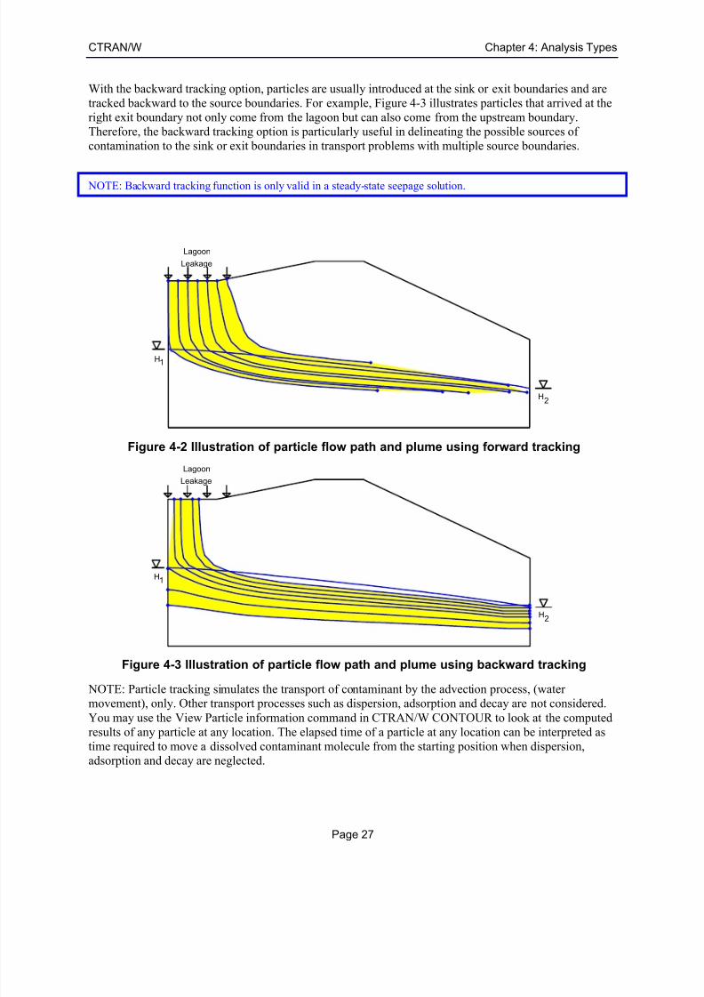
CTRAN/W Chapter 4: Analysis Types
Page 27
With the backward tracking option, particles are usually introduced at the sink or exit boundaries and are
tracked backward to the source boundaries. For example, Figure 4-3 illustrates particles that arrived at the
right exit boundary not only come from the lagoon but can also come from the upstream boundary.
Therefore, the backward tracking option is particularly useful in delineating the possible sources of
contamination to the sink or exit boundaries in transport problems with multiple source boundaries.
NOTE: Backward tracking function is only valid in a steady-state seepage solution.
Figure 4-2 Illustration of particle flow path and plume using forward tracking
Figure 4-3 Illustration of particle flow path and plume using backward tracking
NOTE: Particle tracking simulates the transport of contaminant by the advection process, (watermovement), only. Other transport processes such as dispersion, adsorption and decay are not considered.
You may use the View Particle information command in CTRAN/W CONTOUR to look at the computed
results of any particle at any location. The elapsed time of a particle at any location can be interpreted as
time required to move a dissolved contaminant molecule from the starting position when dispersion,
adsorption and decay are neglected.
Lagoon
Leakage
H1
2H
Lagoon
Leakage
H1
2H

7/25/2019 Ctran Modeling
http://slidepdf.com/reader/full/ctran-modeling 36/101
Chapter 4: Analysis Types CTRAN/W
Page 28
4.4 Adv ect ion-dispers ion analys is
Advection refers to the process by which solutes are transported by the bulk motion of flowing
groundwater. Dispersion refers to the phenomenon of contaminant spreading from the path that it would
be expected to follow according to the advective hydraulics of the flow system. Virtually all contaminant
transport analyses require computation of advection and dispersion.
Adsorption refers to contaminant adsorption onto the solids of the porous medium. Decay refers to
removal of the contaminant by some form of decay reaction, such as radioactive decay. Reactive,
(adsorbing), or decaying contaminants may have a significant effect on the contaminant concentration in
groundwater.
4.5 Density -dependent analysis (with SEEP/W on ly)
For problems where the density of the contaminant is significantly different than water, CTRAN/W has
the capability of performing density-dependent transport analyses. This feature is useful for solving
problems such as sea water intrusion, brine transport and landfill leachate migration, among others.
Contaminant density is modeled as varying linearly with concentration. Contaminant density can be
lower, higher or equal to the density of the native groundwater.
In density-dependent transport analyses, the flow velocities are dependent on the contaminant
concentration distribution and the concentrations are dependent on the flow velocities. This circular
dependence, or non-linearity, requires that the seepage flow velocities and the contaminant concentrations
be solved for simultaneously by iterating at each time step. This type of non-linearity does not exist for
advection-dispersion transport analyses, where the flow velocities are independent of the contaminant
concentration distribution. For advection-dispersion analyses, the seepage velocities may be computed for
all time steps before calculating the contaminant transport.
To allow for the seepage velocities to be calculated at each time step during a density-dependent analysis,
CTRAN/W SOLVE starts and controls an instance of SEEP/W SOLVE to perform the velocity
calculations at each time step. Therefore to perform a density-dependent transport analysis using
CTRAN/W, you must select the analysis type as Density-Dependent in both SEEP/W and CTRAN/W.
In SEEP/W DEFINE you must specify the relative density of the contaminant at a specified reference
concentration. The relative density refers to the density of contaminated water at the specified reference
contaminant concentration. The density of the contaminated water is assumed to vary linearly with
increasing contaminant concentration.
A relative density larger than 1.0 means the contaminant has a higher density than water. Similarly, a
relative density smaller than 1.0 means the contaminant has a lower density than water. By default, the
relative density of the contaminant is 1.0, meaning that there is no density contrast between freshwater
and contaminated water as a function of concentration. Doing a density-dependent analysis with relative
density equal to 1.0 is essentially the same as doing an advection-dispersion transport analysis, except that
the seepage velocities will be re-calculated within each iteration.
The time step increments specified in CTRAN/W DEFINE are used in the analysis for both SEEP/W and
CTRAN/W. Time step information defined in SEEP/W DEFINE is ignored in a density-dependent
analysis. Similarly, the maximum number of iterations allowed within a time step is specified in
CTRAN/W DEFINE. The maximum number of iterations specified in SEEP/W is not used in
density-dependent analyses.
It is important to recognize that the interpretation of head potentials in the seepage solution of a density-
dependent transport problem is somewhat different than the usual interpretation in an advection-

7/25/2019 Ctran Modeling
http://slidepdf.com/reader/full/ctran-modeling 37/101
CTRAN/W Chapter 4: Analysis Types
Page 29
dispersion (density-independent), transport problem. For density-dependent analyses, the total head at a
node is interpreted as the equivalent freshwater head. As the name implies, equivalent freshwater head is
an equivalent total head potential of freshwater. The density contrast between contaminated water and
freshwater adds a “body force” term on the finite elements in the mesh. Therefore if density of the
contaminated water relative to freshwater increases with concentration (relative density greater than 1.0 at
some concentration), then the equivalent freshwater head will increase with contaminant concentration.
Similarly, if the density of the contaminated water relative to freshwater decreases with concentration,(relative density less than 1.0 at some concentration), then the equivalent freshwater head will decrease
with contaminant concentration.
A good example to illustrate the equivalent freshwater head is the static saltwater column example in the
chapter on Illustrative Examples. Although there is an upward gradient in the equivalent freshwater head
within the column, the upward gradient is balanced exactly by the downward gradient caused by the body
force. As a result, there is no flow in the column.
4.6 Problem geometry orientat ion
The orientation of the defined problem in CTRAN/W will depend on what it was specified as in the
SEEP/W or VADOSE/W problem. More detailed discussion of each type of view is provided in thoseother engineering books. A brief review of the possible types of geometry views follows.
Ax isymmet r i c v iew
An axisymmetric analysis can be used to simulate three-dimensional problems with symmetry about a
vertical axis of rotation. The problem is defined in two dimensions, but for analysis, it is as if the section
is rotated about a vertical central axis.
For an axisymmetric analysis, the computed mass flux is per unit radian if the element thickness is
specified as 1.0. If you want the computed flux value for the entire circumferential area, you must either
specify the element thickness as 6.2832 (i.e., 2 pi radians) before you do the analysis, or simply multiply
the above value by 2 pi after the solution is finished. You can change the element thickness for the entire
mesh with the Draw Element Properties command.
Plan view
A plan view analysis views the finite element mesh as lying on its side instead of standing upright in a
vertical plane. In CTRAN/W the only difference between a plan view and a 2D view analysis is the way
the area of a unit “q” contaminant mass flux boundary is computed.
In a plan view, the area by which the “q” contaminant mass flux rate is multiplied comes from the plan
view areas of each element that contribute data to the “q” specified nodes. The solver will compute the
element areas and apply the flux, Q, to the nodes.
2D view
In a 2D view, the area by which the “q” contaminant mass flux rate is multiplied comes from the length of
the element edges that the boundary condition is specified. This length is then multiplied by the specified
thickness of the element (typically unit thickness into the screen) to obtain a total flux, Q, to apply at the
relevant nodes.
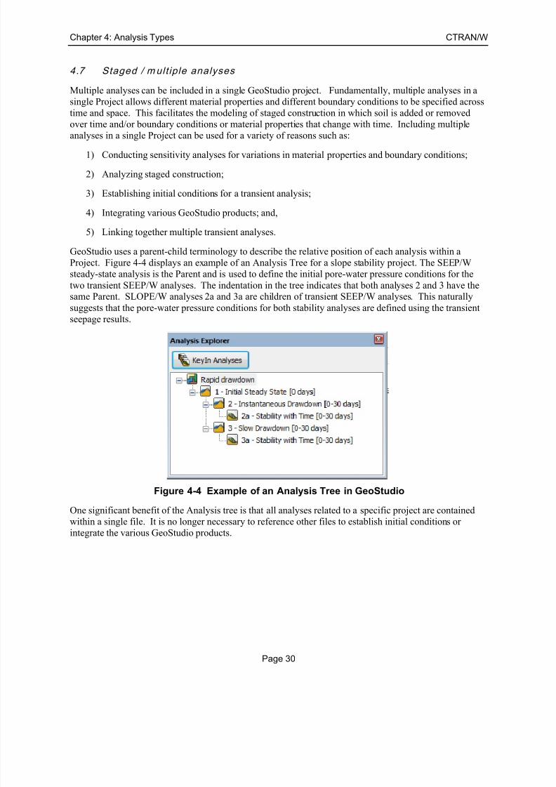
7/25/2019 Ctran Modeling
http://slidepdf.com/reader/full/ctran-modeling 38/101
Chapter 4: Analysis Types CTRAN/W
Page 30
4.7 Staged / mult iple analyses
Multiple analyses can be included in a single GeoStudio project. Fundamentally, multiple analyses in a
single Project allows different material properties and different boundary conditions to be specified across
time and space. This facilitates the modeling of staged construction in which soil is added or removed
over time and/or boundary conditions or material properties that change with time. Including multiple
analyses in a single Project can be used for a variety of reasons such as:
1) Conducting sensitivity analyses for variations in material properties and boundary conditions;
2) Analyzing staged construction;
3) Establishing initial conditions for a transient analysis;
4) Integrating various GeoStudio products; and,
5) Linking together multiple transient analyses.
GeoStudio uses a parent-child terminology to describe the relative position of each analysis within a
Project. Figure 4-4 displays an example of an Analysis Tree for a slope stability project. The SEEP/W
steady-state analysis is the Parent and is used to define the initial pore-water pressure conditions for thetwo transient SEEP/W analyses. The indentation in the tree indicates that both analyses 2 and 3 have thesame Parent. SLOPE/W analyses 2a and 3a are children of transient SEEP/W analyses. This naturally
suggests that the pore-water pressure conditions for both stability analyses are defined using the transient
seepage results.
Figure 4-4 Example of an Analysis Tree in GeoStudio
One significant benefit of the Analysis tree is that all analyses related to a specific project are contained
within a single file. It is no longer necessary to reference other files to establish initial conditions or
integrate the various GeoStudio products.

7/25/2019 Ctran Modeling
http://slidepdf.com/reader/full/ctran-modeling 39/101
CTRAN/W Chapter 4: Analysis Types
Page 31

7/25/2019 Ctran Modeling
http://slidepdf.com/reader/full/ctran-modeling 40/101
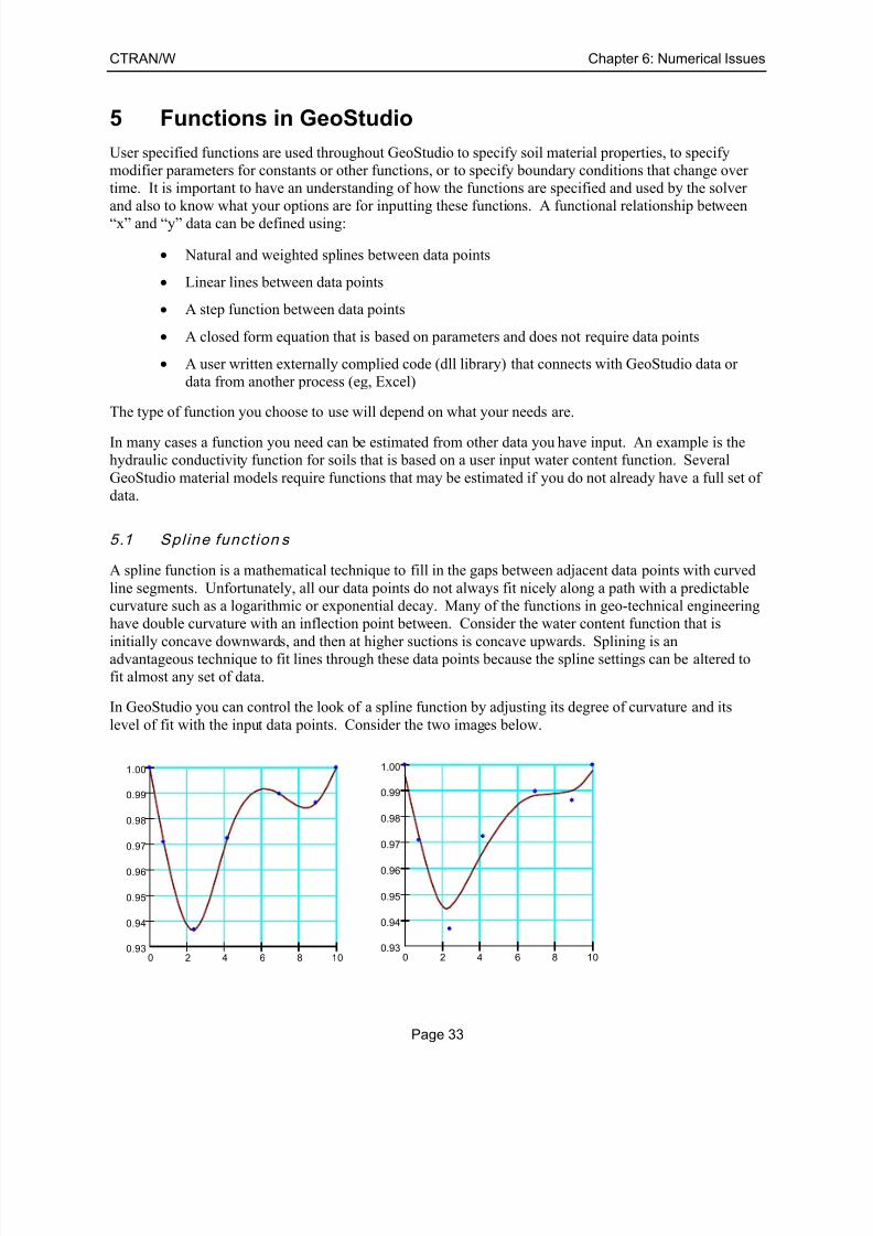
7/25/2019 Ctran Modeling
http://slidepdf.com/reader/full/ctran-modeling 41/101
CTRAN/W Chapter 6: Numerical Issues
Page 33
5 Functions in GeoStudio
User specified functions are used throughout GeoStudio to specify soil material properties, to specify
modifier parameters for constants or other functions, or to specify boundary conditions that change over
time. It is important to have an understanding of how the functions are specified and used by the solver
and also to know what your options are for inputting these functions. A functional relationship between
“x” and “y” data can be defined using:
• Natural and weighted splines between data points
• Linear lines between data points
• A step function between data points
• A closed form equation that is based on parameters and does not require data points
• A user written externally complied code (dll library) that connects with GeoStudio data or
data from another process (eg, Excel)
The type of function you choose to use will depend on what your needs are.
In many cases a function you need can be estimated from other data you have input. An example is the
hydraulic conductivity function for soils that is based on a user input water content function. Several
GeoStudio material models require functions that may be estimated if you do not already have a full set of
data.
5.1 Spl ine funct ion s
A spline function is a mathematical technique to fill in the gaps between adjacent data points with curved
line segments. Unfortunately, all our data points do not always fit nicely along a path with a predictable
curvature such as a logarithmic or exponential decay. Many of the functions in geo-technical engineering
have double curvature with an inflection point between. Consider the water content function that is
initially concave downwards, and then at higher suctions is concave upwards. Splining is anadvantageous technique to fit lines through these data points because the spline settings can be altered to
fit almost any set of data.
In GeoStudio you can control the look of a spline function by adjusting its degree of curvature and its
level of fit with the input data points. Consider the two images below.
0.93
0.94
0.95
0.96
0.97
0.98
0.99
1.00
0 2 4 6 8 100.93
0.94
0.95
0.96
0.97
0.98
0.99
1.00
0 2 4 6 8 10

7/25/2019 Ctran Modeling
http://slidepdf.com/reader/full/ctran-modeling 42/101
Chapter 6: Numerical Issues CTRAN/W
Page 34
Figure 5-1 Spline functions with different settings
The left image has the spline fit almost exactly through the data points with fairly curved segments. The
right image has more linear segments that only fit the data approximately. The range of fit and curvatureis controlled by two “slider controls” and can range between values of zero and 100%. The important
thing to note is that the solver will use the data represented by the splined fit. What you see in the
function set up is EXACTLY what the solver will use when needed.
Slopes of spl ine funct ions
Sometimes, the solver does not require the “Y” value of a function at a given “X” value but the slope of
the function at a given “X” value. This is the case for the water content function where the slope is useddirectly in the solution of the transient seepage and air flow equations. You must be careful when setting
spline values because while a spline may look smooth, its slope may not be so.
The two images below are the slopes of the two functions shown above. You can see that the more
natural curved function (left side images) with 100% curvature and exactness in the spline settings
produces a much smoother slope function than the approximated function. While not usually critical, you
should know if the function you are using is dependent on its slope being well behaved.
Figure 5-2 Slope of spline functions
5.2 Linear funct ion s
A linear function is a spline function with the curvature setting to 0% and the fit set to 100% exact as
shown below.
-0.01
-0.03
-0.04
0.00
0.01
0.03
0.04
0 2 4 6 8 10
-0.02
-0.03
-0.05
0.00
0.02
0.03
0 2 4 6 8 10
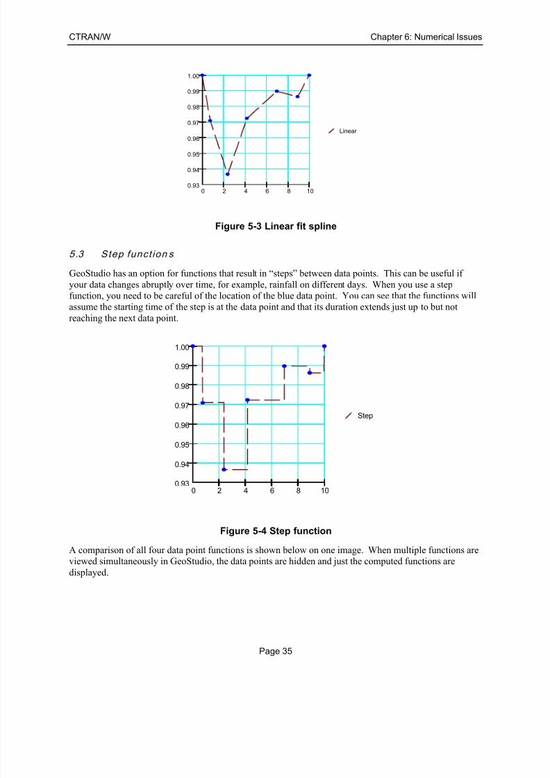
7/25/2019 Ctran Modeling
http://slidepdf.com/reader/full/ctran-modeling 43/101
CTRAN/W Chapter 6: Numerical Issues
Page 35
Figure 5-3 Linear fit spline
5.3 Step funct ion s
GeoStudio has an option for functions that result in “steps” between data points. This can be useful if
your data changes abruptly over time, for example, rainfall on different days. When you use a step
function, you need to be careful of the location of the blue data point. You can see that the functions will
assume the starting time of the step is at the data point and that its duration extends just up to but not
reaching the next data point.
Figure 5-4 Step function
A comparison of all four data point functions is shown below on one image. When multiple functions are
viewed simultaneously in GeoStudio, the data points are hidden and just the computed functions are
displayed.
Linear
0.93
0.94
0.95
0.96
0.97
0.98
0.99
1.00
0 2 4 6 8 10
Step
0.93
0.94
0.95
0.96
0.97
0.98
0.99
1.00
0 2 4 6 8 10
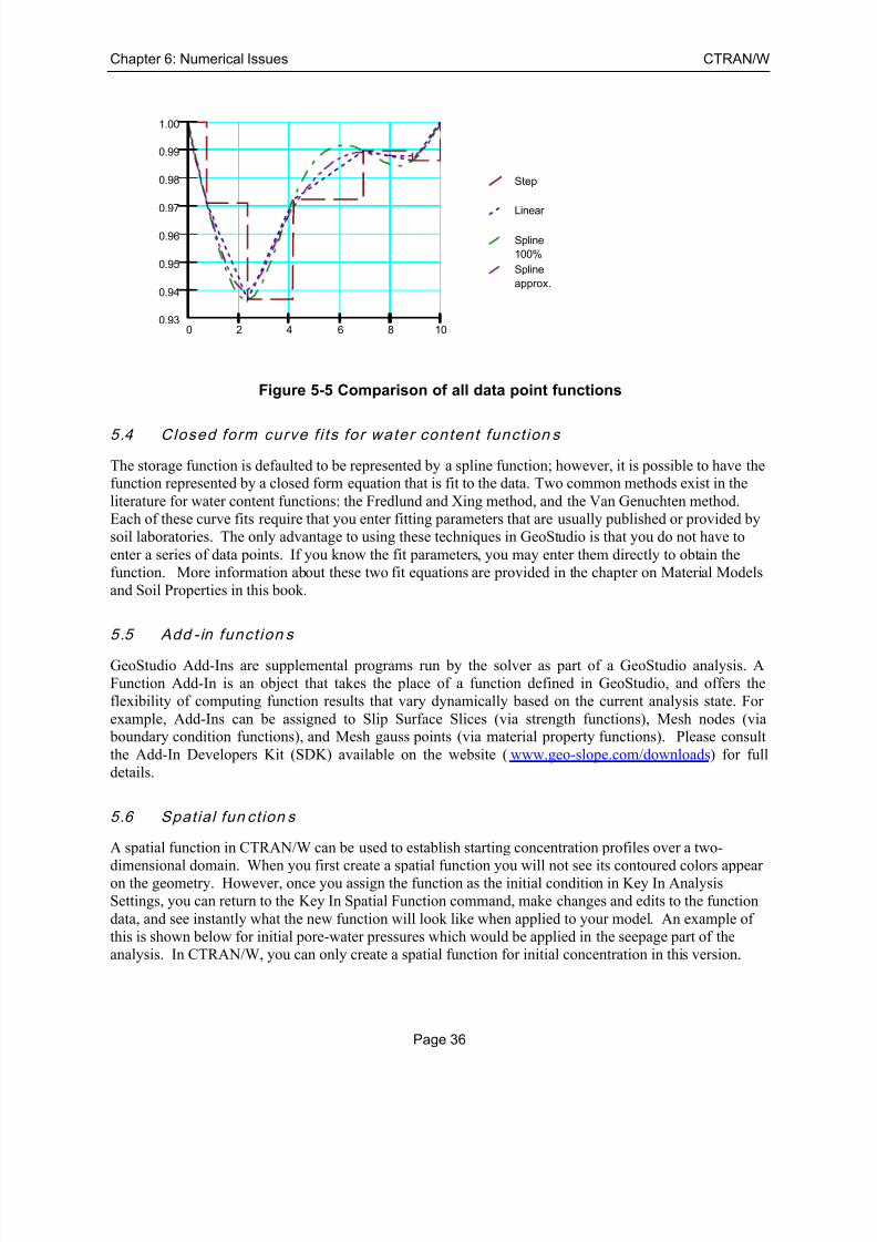
7/25/2019 Ctran Modeling
http://slidepdf.com/reader/full/ctran-modeling 44/101
Chapter 6: Numerical Issues CTRAN/W
Page 36
Figure 5-5 Comparison of all data point functions
5.4 Closed form curve f i ts for water content funct ion s
The storage function is defaulted to be represented by a spline function; however, it is possible to have thefunction represented by a closed form equation that is fit to the data. Two common methods exist in the
literature for water content functions: the Fredlund and Xing method, and the Van Genuchten method.
Each of these curve fits require that you enter fitting parameters that are usually published or provided by
soil laboratories. The only advantage to using these techniques in GeoStudio is that you do not have to
enter a series of data points. If you know the fit parameters, you may enter them directly to obtain the
function. More information about these two fit equations are provided in the chapter on Material Models
and Soil Properties in this book.
5.5 Add -in funct ion s
GeoStudio Add-Ins are supplemental programs run by the solver as part of a GeoStudio analysis. A
Function Add-In is an object that takes the place of a function defined in GeoStudio, and offers the
flexibility of computing function results that vary dynamically based on the current analysis state. For
example, Add-Ins can be assigned to Slip Surface Slices (via strength functions), Mesh nodes (via boundary condition functions), and Mesh gauss points (via material property functions). Please consult
the Add-In Developers Kit (SDK) available on the website (www.geo-slope.com/downloads) for full
details.
5.6 Spatial fun ction s
A spatial function in CTRAN/W can be used to establish starting concentration profiles over a two-
dimensional domain. When you first create a spatial function you will not see its contoured colors appearon the geometry. However, once you assign the function as the initial condition in Key In Analysis
Settings, you can return to the Key In Spatial Function command, make changes and edits to the function
data, and see instantly what the new function will look like when applied to your model. An example of
this is shown below for initial pore-water pressures which would be applied in the seepage part of the
analysis. In CTRAN/W, you can only create a spatial function for initial concentration in this version.
Step
Linear
Spline
100%
Spline
approx.
0.93
0.94
0.95
0.96
0.97
0.98
0.99
1.00
0 2 4 6 8 10
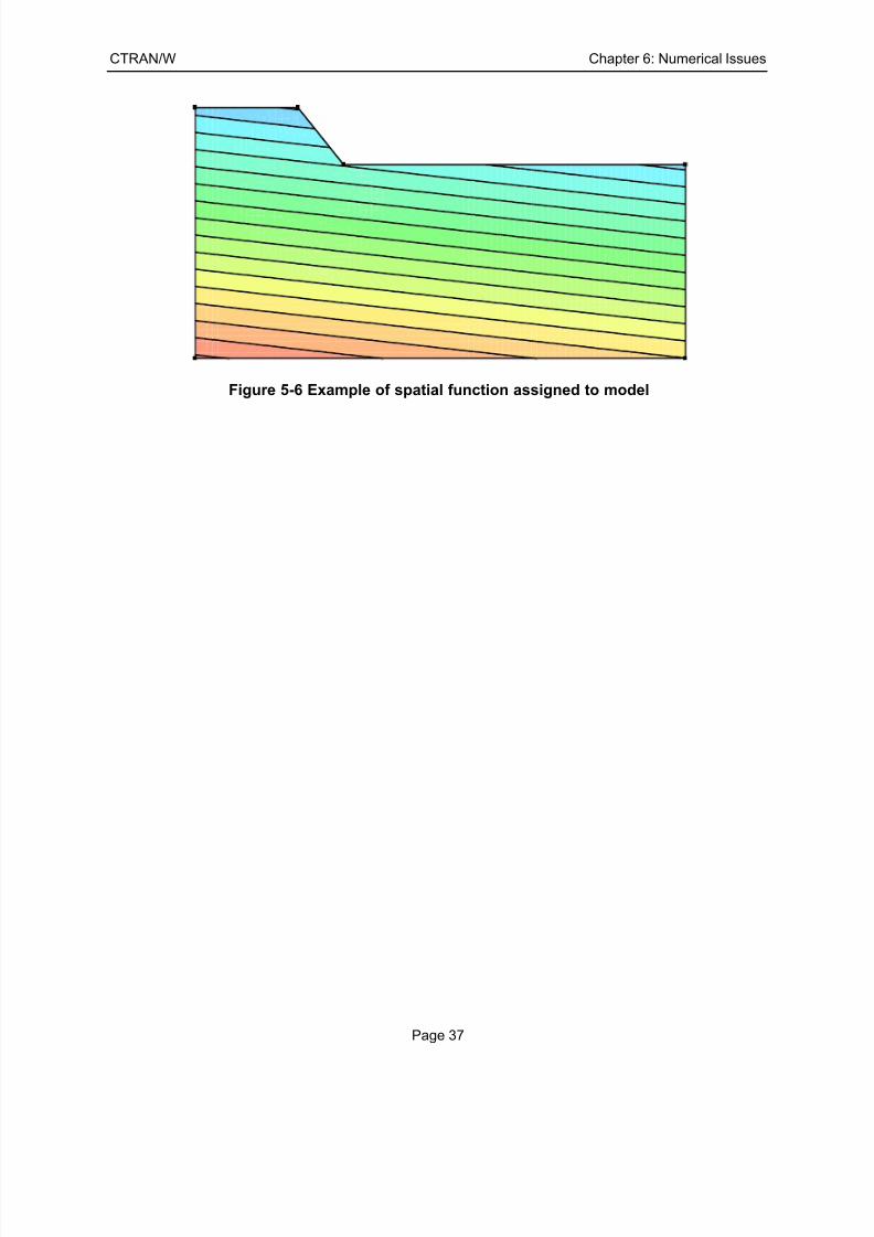
7/25/2019 Ctran Modeling
http://slidepdf.com/reader/full/ctran-modeling 45/101
CTRAN/W Chapter 6: Numerical Issues
Page 37
Figure 5-6 Example of spatial function assigned to model

7/25/2019 Ctran Modeling
http://slidepdf.com/reader/full/ctran-modeling 46/101
Chapter 6: Numerical Issues CTRAN/W
Page 38
7/25/2019 Ctran Modeling
http://slidepdf.com/reader/full/ctran-modeling 47/101
CTRAN/W Chapter 6: Numerical Issues
Page 39
6 Numerical Issues
Entire textbooks can be written on numerical issues related to finite element analysis. While modern
computers and powerful graphics can make defining an analysis quite fast and easy, they can not
necessarily deal with some of the intricate issues related to the concept of taking a natural process and
breaking it down into finite time and special domains (i.e. individual elements within a soil geometry).
There are various ways to deal with many of the numerical issues, but the unfortunate part is that there is
no single method, approach, or technique that can deal with all problems. Some numerical issues relate to
restrictions in computer hardware such as rounding off of non-integer variables during math operations;
some issues relate to non-linearity of soil properties; some issues relate to the fact the physical equations
being solved do not apply to all cases (for example, CTRAN/W does not account for contaminants
moving in both the air and liquid phases); some issues relate to our inability to discretize a domain to
small enough element sizes; and other issues relate to the fact we have made the elements too small!
There are numerical solvers that make use of adaptive meshing or adaptive time stepping or both in
attempts to be more suited to a wider range of problems. All of these, however, have their limitations
from a sound mathematical perspective – regardless of what the software developer will tell you. If you
don’t know what the limitations are, it becomes somewhat risky to rely on a solver that claims to “handleit all.”
Some finite element solutions attempt to march forward in time by considering soil property values taken
from the last, the current or the mid-time step average. Some solvers simply make assumptions that limit
their applicability to real life in order to get a solution, such as moving the mesh to find the water table in
a seepage program instead of solving for the physics of flow above and below the water table. Finally,
some solvers may only work if you put in an initial guess of the solution for the dependent variable being
solved that is close to the desired solution, in other words, start off the solution by pointing it in the right
direction.
While it may appear all hope is lost, this is far from the case. Sound judgment and common sense can
usually overcome most of these challenges and result in meaningful interpretations of how the soil will
respond to changes in various parameters.
It is not always possible to get an exact solution in many challenging cases, so you should not necessarily
be seeking an exact solution. If the problem is so difficult that it is not solving reasonably, then it is very
likely that either mistakes have been made in the input, or, that you are pushing the envelope of the
physical theory applied in the model. This chapter looks at some of these issues as they pertain to
CTRAN/W.
6.1 Convergence
The objective of solving the finite element equations is to compute the concentration at each node. For
linear analyses when the material properties are constant, the nodal concentrations can be computed
directly. However, in the cases of nonlinear analyses where there is adsorption as a function ofconcentration, the correct material properties are not known at the start of the analysis; consequently, an
iterative scheme is required to solve the equations.
CTRAN/W uses a repeated substitution technique in the iterative process. For the first iteration, the user-
specified initial concentrations are used to define the material properties. The material properties are
updated in subsequent iterations using the computed concentration from the previous iteration. The
iterative process continues until the iteration number reaches the maximum number specified or until the
results satisfy the convergence criteria.

7/25/2019 Ctran Modeling
http://slidepdf.com/reader/full/ctran-modeling 48/101
Chapter 6: Numerical Issues CTRAN/W
Page 40
Convergence means repeated solving of the nodal transport equations until the computed solution does
not change by more than a specified amount on successive iterations. If the equations want to solve to the
same results over and over, then this means that the soil property values used in the solution agree with
the computed concentration values at each position in the mesh, and that the influence of the boundary
conditions (i.e., adding or removing mass) also are reflected in the correct soil properties and
concentrations. Everything must be just right to balance both sides of the transport equation.
Vector norm s
CTRAN/W does not use individual nodal concentrations to make the comparison between successive
iterations. Instead, it uses the percent change in the vector norm – a process that considers all nodal
concentrations simultaneously. The vector norm is computed as the square root of the sum of each nodal
concentration value squared, or in equation form:
2
1
n
i
i
N C =
=
where:
N = the vector norm,
i = a counter,
n = the total number of nodes, and
iC = the individual nodal concentrations.
The percent change in the vector norm is simply the change in the value N between two successive
iterations. If the change in N were exactly zero, then there would be no change in solution on successive
iterations. In general, there are always very small differences between iterations so it is not reasonable to
expect a change in vector norm of zero.
You may wonder why we use the vector norm. It is a powerful way of considering the entire problem in a
single comparison, which prevents any individual nodal concentration from potentially failing the
convergence test in a solution that really should be considered converged.
When the dependent variable (e.g. concentration in a transport analysis) gets close to zero, very small
changes in a single variable between successive iterations can appear to be very big when converted to a
percent difference comparison. Consider if a single nodal concentration is changing from 0.01 to 0.02
between successive iterations. This is a change of 100% but likely insignificant from a physical
perspective. It’s a failure in the logic of checking convergence by individual nodal percent difference,
because it lets small physical changes become significant mathematical changes.
During the iterative process, CTRAN/W calculates the percent difference in vector norm; which
represents the percent difference in the concentration of all nodes between two consecutive iterations. Inan analysis where there is no adsorption or in a particle tracking analysis, the problem is linear and is
solved in one iteration. Consequently, convergence parameters are ignored.
6.2 Numerical dispers ion and osci l lat ion
Numerical dispersion and oscillation are inherent in the finite element solution of the
advection-dispersion equation. The two phenomena are illustrated graphically in Figure 6-1. Numerical

7/25/2019 Ctran Modeling
http://slidepdf.com/reader/full/ctran-modeling 49/101
CTRAN/W Chapter 6: Numerical Issues
Page 41
dispersion tends to spread out the contaminant more than what is predicted by analytical solutions.
Numerical oscillation produces concentrations higher or lower than the maximum and minimum specified
values.
Figure 6-1 The phenomena of numerical dispersion and oscillation
Numerical dispersion and oscillation cannot be eliminated; they can only be controlled or minimized. The
two widely used criteria are the Peclet Number and the Courant number constraints. (See Frind and
Pinder, 1982, and Daus, Frind and Sudicky, 1983).
6.3 Peclet and Courant num ber cri ter ia
The Peclet and Courant Number criteria are usually expressed in the one-dimensional form as follows:
Peclet Number = 2v x
D
∆≤
Courant Number = 1v t
x
∆≤
∆
where:
∆ = nodal spacing,
D = hydrodynamic dispersion coefficient,
ν = average linear velocity, and
t ∆ = incremental time step.
In two-dimensional analyses, CTRAN/W computes the Peclet and Courant Numbers at each Gauss point
of an element using the following equations:
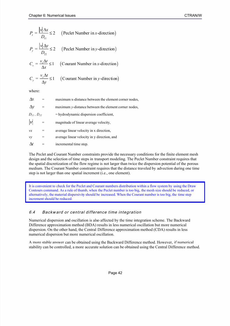
7/25/2019 Ctran Modeling
http://slidepdf.com/reader/full/ctran-modeling 50/101
Chapter 6: Numerical Issues CTRAN/W
Page 42
( )11
= 2 Peclet Number in -direction x
v x P x
D
∆≤
( )22
= 2 Peclet Number in -direction y
v y P y
D
∆≤
( )= 1 Courant Number in -direction x x
v t C x
x
∆≤
∆
( )= 1 Courant Number in -direction y
y
v t C y
y
∆≤
∆
where:
∆ = maximum x-distance between the element corner nodes,
y∆ = maximum y-distance between the element corner nodes,
D11 , D22 = hydrodynamic dispersion coefficient,
ν = magnitude of linear average velocity,
vx = average linear velocity in x direction,
vy = average linear velocity in y direction, and
t ∆ = incremental time step.
The Peclet and Courant Number constraints provide the necessary conditions for the finite element mesh
design and the selection of time steps in transport modeling. The Peclet Number constraint requires that
the spatial discretization of the flow regime is not larger than twice the dispersion potential of the porous
medium. The Courant Number constraint requires that the distance traveled by advection during one timestep is not larger than one spatial increment (i.e., one element).
It is convenient to check for the Peclet and Courant numbers distribution within a flow system by using the DrawContours command. As a rule of thumb, when the Peclet number is too big, the mesh size should be reduced, or
alternatively, the material dispersivity should be increased. When the Courant number is too big, the time step
increment should be reduced.
6.4 Backward or central di f ference t ime integrat ion
Numerical dispersion and oscillation is also affected by the time integration scheme. The Backward
Difference approximation method (BDA) results in less numerical oscillation but more numericaldispersion. On the other hand, the Central Difference approximation method (CDA) results in less
numerical dispersion but more numerical oscillation.
A more stable answer can be obtained using the Backward Difference method. However, if numerical
stability can be controlled, a more accurate solution can be obtained using the Central Difference method.

7/25/2019 Ctran Modeling
http://slidepdf.com/reader/full/ctran-modeling 51/101
CTRAN/W Chapter 6: Numerical Issues
Page 43
In summary, it is best to start with the more stable Backward Difference method and then refine the
solution with the Central Difference method once all other factors in the analysis have been modeled
correctly. In many cases, the differences between the two methods are relatively small.
6.5 Mesh desig n
The Meshing chapter of the SEEP/W or VADOSE/W books provides general modeling guidelines for the
design of a finite element mesh for seepage analysis. This section provides additional guidelines which
should be followed in order to extend the seepage analysis results for contaminant transport modeling.
In order to obtain stable solutions in a transport analysis, both the Peclet Number and Courant number
criteria must be considered in the design of the finite element mesh. Rearranging the above Peclet and
Courant number equations, the spatial discretization requirements are:
11 2 D
xv
∆ ≤
22
2
D
y v∆ ≤
x x v t ∆ ≤ ∆
y y v t ∆ ≤ ∆
The above equations indicate that the spatial discretization of the flow regime should not be larger than
twice the dispersion potential of the porous medium and the distance traveled by advection during one
time step. In most cases, the time steps can be easily reduced to satisfy the Courant criterion, therefore,
the design of the mesh depending primarily on the seepage velocity and the dispersivity of the materials.
Since the equations require knowledge of the average linear velocity, the Peclet and Courant Numbers for
each element will not be known at the time you create the finite element mesh. Therefore, these criteriacannot be rigidly applied during creation of the mesh. As a broad rule, the discretization in the major flow
direction should be about twice the longitudinal dispersivity Lα of the soil, and the discretization in the
minor flow direction should be about twice the transverse dispersivity T α of the soil.
This will provide a starting point for you to estimate the required spatial discretization. Later, you can
confirm the actual Peclet and Courant Numbers computed by CTRAN/W and check that both the Peclet
and Courant Number criteria are satisfied in all time steps.
6.6 Time step design
Numerical dispersion and oscillation are directly affected by the time step increments. To minimizenumerical dispersion and oscillation, the Courant Number constraint should be satisfied. The Courant
Number constraint requires that the distance traveled by the advective component of the transport process
during one time step ideally should not be larger than one element; that is, the advective component
should not jump across elements in one time step.
In order to satisfy the Courant Number constraint, the time increment should be:
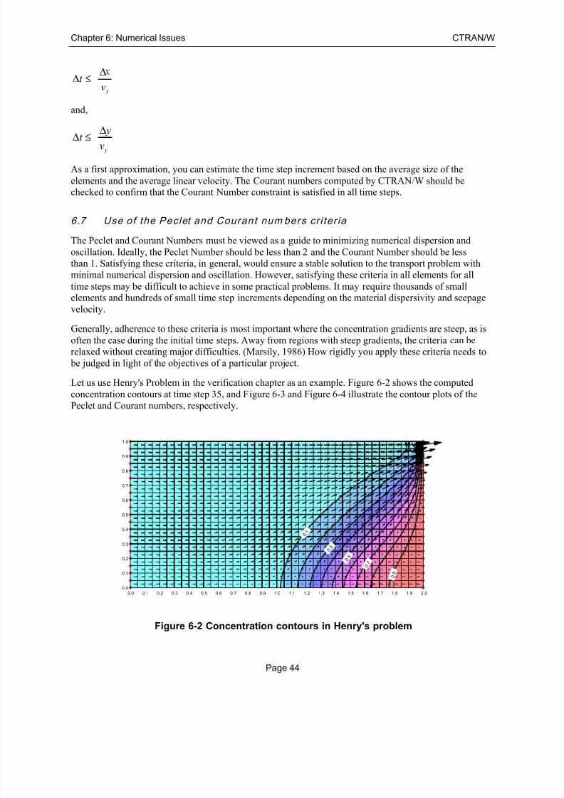
7/25/2019 Ctran Modeling
http://slidepdf.com/reader/full/ctran-modeling 52/101
Chapter 6: Numerical Issues CTRAN/W
Page 44
x
t v
∆∆ ≤
and,
y
yt v
∆
∆ ≤
As a first approximation, you can estimate the time step increment based on the average size of the
elements and the average linear velocity. The Courant numbers computed by CTRAN/W should bechecked to confirm that the Courant Number constraint is satisfied in all time steps.
6.7 Use of the Peclet and Courant num bers cri ter ia
The Peclet and Courant Numbers must be viewed as a guide to minimizing numerical dispersion and
oscillation. Ideally, the Peclet Number should be less than 2 and the Courant Number should be less
than 1. Satisfying these criteria, in general, would ensure a stable solution to the transport problem with
minimal numerical dispersion and oscillation. However, satisfying these criteria in all elements for alltime steps may be difficult to achieve in some practical problems. It may require thousands of smallelements and hundreds of small time step increments depending on the material dispersivity and seepage
velocity.
Generally, adherence to these criteria is most important where the concentration gradients are steep, as is
often the case during the initial time steps. Away from regions with steep gradients, the criteria can be
relaxed without creating major difficulties. (Marsily, 1986) How rigidly you apply these criteria needs to
be judged in light of the objectives of a particular project.
Let us use Henry's Problem in the verification chapter as an example. Figure 6-2 shows the computed
concentration contours at time step 35, and Figure 6-3 and Figure 6-4 illustrate the contour plots of the
Peclet and Courant numbers, respectively.
Figure 6-2 Concentration contours in Henry's problem
0 . 1
0 . 3
0 . 5
0 . 7
0 . 9
0.0 0.1 0.2 0.3 0.4 0.5 0.6 0.7 0.8 0.9 1.0 1.1 1.2 1.3 1.4 1.5 1.6 1.7 1.8 1.9 2.00.0
0.1
0.2
0.3
0.4
0.5
0.6
0.7
0.8
0.9
1.0

7/25/2019 Ctran Modeling
http://slidepdf.com/reader/full/ctran-modeling 53/101
CTRAN/W Chapter 6: Numerical Issues
Page 45
Figure 6-3 Peclet number contours of Henry's problem
Figure 6-4 Courant number contours of Henry's problem
Near the upper right corner of the flow system, where the seepage velocity is the highest, both the Peclet
and Courant numbers criteria are not satisfied. However, within most of the flow system, the Peclet
number criterion is satisfied and the Courant number is slightly higher than the suggested criterion. As a
result, the concentration contours indicate that a stable solution was obtained within most of the flow
system, and a small area with numerical instability is observed near the upper right corner. The numericalinstability causes small negative concentration values to be computed at the upper nodes between the 0.1
and 0.2 concentration contour lines. The concentration contours greater than 0.3 are not significantly
affected by the instability.
It is possible to improve the simulation such that both the Peclet and Courant number criteria are satisfied
and numerical instability is minimized. To do so will require substantial refinement to the mesh especially
in the upper right corner, and a much finer time step increment. Since the area of interest of the Henry’s
0. 2
0. 4
0 .6
1
1 .4
1 .8
0.0 0.1 0.2 0.3 0.4 0.5 0.6 0.7 0.8 0.9 1.0 1.1 1.2 1.3 1.4 1.5 1.6 1.7 1.8 1.9 2.00.0
0.1
0.2
0.3
0.4
0.5
0.6
0.7
0.8
0.9
1.0
1
1
3
5
7
0.0 0.1 0.2 0.3 0.4 0.5 0.6 0.7 0.8 0.9 1.0 1.1 1.2 1.3 1.4 1.5 1.6 1.7 1.8 1.9 2.00.0
0.1
0.2
0.3
0.4
0.5
0.6
0.7
0.8
0.9
1.0

7/25/2019 Ctran Modeling
http://slidepdf.com/reader/full/ctran-modeling 54/101
Chapter 6: Numerical Issues CTRAN/W
Page 46
problem is in the lower right portion of the flow system, and only the 0.5 concentration contour line is
used in the comparison with other models, we feel that it is not necessary to further refine the analysis.
6.8 Gauss integrat ion order
The details of numerical integration are provided in the appendices, along with a discussion of how
different integration orders can affect results for various types of elements. Part of this discussion is
repeated here as it pertains to improving solution convergence.
The appropriate integration order is a function of the presence of secondary nodes. When secondary nodes
are present, the interpolating functions are nonlinear and consequently a higher integration order is
required. Table 6-1 gives the acceptable integration orders.
Table 6-1 Acceptable element integration orders
Element Type Secondary Nodes Integration Order
Quadrilateral no 4
Quadrilateral yes 9
Triangular no 1
Triangular yes 3
It is also acceptable to use four-point integration for quadrilateral elements which have secondary nodes.
This is called a reduced integration order (see Bathe, 1982). Acceptable results can be obtained with
reduced integration.
It is also possible to use three-point and nine-point integration with elements that have no secondary
nodes. However, the benefits of this are marginal, particularly for quadrilateral elements. Nine-point
integration for a quadrilateral element involves substantially more computing than four-point integration,
and there is little to be gained from the additional computations. As a general rule, quadrilateral elements
should have secondary nodes to achieve significant benefits from the nine-point integration.
The situation is slightly different for triangular elements. One-point integration means the material
properties and flow gradients are constant within the element. This can lead to poor performance of the
element, particularly if the element is a zone of steep concentration gradient and there is active
adsorption. Using three-point integration, even without using secondary nodes, can improve the
performance, since material properties and gradients within the elements are distributed in a more realistic
manner. The use of three-point integration in triangular elements with no secondary nodes is considered
acceptable for triangular elements in a mesh that has predominantly quadrilateral elements. This approach
is not recommended if the mesh consists primarily of triangular elements with no secondary nodes.
In general, it is sufficient to use three-point integration for triangular elements and four-point integration
for quadrilateral elements. In situations where there is adsorption and steep gradients within an element, it
is best to use quadrilateral elements with secondary nodes together with nine-point integration.
6.9 Equatio n solv ers (direct or paral lel direct)
CTRAN/W has two types of equation solvers built into it; a direct equation solver and a parallel direct
equation solver. Both offer certain advantages.
Select the direct equation solver option if you want the system equations to be solved using a Gauss
elimination skyline direct solver. The processing speed of the direct solver is bandwidth (the maximum
7/25/2019 Ctran Modeling
http://slidepdf.com/reader/full/ctran-modeling 55/101
CTRAN/W Chapter 6: Numerical Issues
Page 47
node number difference of all the elements in a domain) dependent. In other words, the direct solver is
very fast when solving simple problems with small bandwidth, but it can be quite slow when solving
more complex problems with a large bandwidth. CTRAN/W automatically sorts the nodes so that the
bandwidth is the smallest possible value, which helps the solution solve faster using the direct solver. By
default, the direct equation solver is selected.
Select the parallel direct equation solver option if you have a larger mesh. The parallel solver will savethe matrices in a compressed format to eliminate zero’s and it has many advanced schemes to solve large
systems of equations more efficiently. It also offers the ability to make use of multiple processors on a
computer if they are available. The disadvantage of this solver is that it is a bit slower when the models
are smaller in size.
If in doubt, try each solver and choose the one that offers the best performance.

7/25/2019 Ctran Modeling
http://slidepdf.com/reader/full/ctran-modeling 56/101
Chapter 6: Numerical Issues CTRAN/W
Page 48

7/25/2019 Ctran Modeling
http://slidepdf.com/reader/full/ctran-modeling 57/101
CTRAN/W Chapter 7: Visualization of Results
Page 49
7 Visualization of Results
When you get to the visualization of results stage of a finite element analysis you can congratulate
yourself for having completed the hardest parts – setting up the geometry, defining meaningful soil
property functions, and applying appropriate boundary conditions to the mesh. If, at this point, you do not
have the tools or the understanding of how to interpret the massive amount of data that may have been
generated by the solver, then you have wasted your time.
This chapter describes the various types of output data that are computed by the solver and it attempts to
get you thinking about what the data is trying to tell you. For example, did the solution solve properly?
Did the boundary conditions you applied get reflected in the actual solution? Did the soil respond how
you thought it would respond? If not, how to you methodically determine what to check next?
The chapter is structured to explain what type of data is available for visualization. In the various
sections, comments are provided that relate they type of result data in question to how is should be used
in the overall thought process. It’s a good idea to read this entire chapter.
7.1 Node and element inform at ion
In order to understand what type of information can be viewed as results output, it helps a bit to know
how the data is obtained. To recap, you set up the problem geometry, define material properties, and
apply boundary conditions of either known concentration or mass flux. The solver assembles the soil
property and geometry information for every Gauss point in every element and applies it to the transport
equation that is written for every node. Therefore, at each node we have some applied boundary data,
some interpolated soil property data and geometry data. The solver then computes the unknown value in
the equation for each node – the unknown value being either concentration or flux. It is the Gauss point
data that is used to set up the nodal equations so the Gauss point data written to the output file is the
actual data used in the solver.
Figure 7-1 is an illustration of the type of information that can be viewed for each node in the finite
element mesh. You can view information about geometry, material properties, seepage results,concentrations and boundary fluxes as well as gradients, water velocities etc. Of significance is the ability
to view Courant and Peclet information. This is discussed more in the contouring data section below.
One key point to note in the figure below is that the nodal Boundary Mass Flux quantity is exactly zero.
This is an important point to understand because it can help with your overall interpretation of results.
This boundary flux is computed by summing the contributing fluxes from each of the four Gauss points
that surround this node. So, if mass is flowing out of one Gauss region, it HAS TO be flowing into an
adjacent Gauss region. For all internal nodes with no user boundary applied to them, the sum of all the
mass fluxes at a node should equal zero in a properly converged solution. In other words, there is mass
balance at the node.

7/25/2019 Ctran Modeling
http://slidepdf.com/reader/full/ctran-modeling 58/101
Chapter 7: Visualization of Results CTRAN/W
Page 50
Figure 7-1 Visualization of node information
If the node being viewed is a boundary condition node (not necessarily at the edge of the geometry but
with an allowed influx or out flux) then the summation of all the mass fluxes at that node will not be zero because contaminant mass is either gained or lost at that point.
Figure 7-2 is the corresponding Gauss point information for the Gauss point located just above and to the
right of the node illustrated in the previous figure. The shaded region in the figure shows the contributing
area of that Gauss point and in this case, because the element is rectangular and has no secondary nodes,
this Gauss area is equal to one fourth of the total area of the element. The inset in the figure below shows
the type of data that can be viewed at each Gauss point. If you consider the water content value of 34.9%,
for example, you should realize that this water content is assumed to exist throughout the Gauss point area
displayed; and you should next realize that if the element size is increased, the estimate of the water
content becomes less accurate as we are averaging it over a larger area. The real trick to getting good
finite element analysis results, is to create a finite element mesh with just the right sized elements that are
not too big or too small, that can represent the highly non-linear soil properties within them, and that can
handle the potentially extreme boundary conditions you apply. It’s not always easy and there is no sure
quick or automatic method to make that happen.
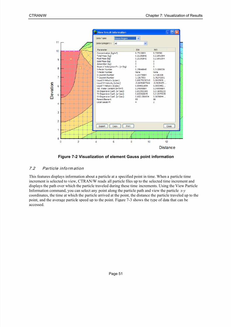
7/25/2019 Ctran Modeling
http://slidepdf.com/reader/full/ctran-modeling 59/101
CTRAN/W Chapter 7: Visualization of Results
Page 51
Figure 7-2 Visualization of element Gauss point information
7.2 Part ic le info rmationThis features displays information about a particle at a specified point in time. When a particle time
increment is selected to view, CTRAN/W reads all particle files up to the selected time increment anddisplays the path over which the particle traveled during these time increments. Using the View Particle
Information command, you can select any point along the particle path and view the particle x- y
coordinates, the time at which the particle arrived at the point, the distance the particle traveled up to the
point, and the average particle speed up to the point. Figure 7-3 shows the type of data that can be
accessed.

7/25/2019 Ctran Modeling
http://slidepdf.com/reader/full/ctran-modeling 60/101
Chapter 7: Visualization of Results CTRAN/W
Page 52
Figure 7-3 View particle information data
The position of the particles is a good indication of where the 50% concentration value will be at any
given time. Consider an advection – dispersion problem where some contaminant is moving due to water
flow; and some is moving ahead of the water due to molecular action, while some is retarded in progress
due to molecular action in the direction opposite to flow. The “s” shape of the concentration plug
illustrates this idea. Now, consider the mid-point of the “s” shape. It is a point in concentration (the 50%
point) and it is moving solely due to advection. So, if we are only interested in the position of the 50%
concentration point, we can simply use a particle tracking analysis and not the full advection – dispersion
solution.
7.3 Mass accumulat ion
This feature displays accumulated mass values within selected elements. In a contaminant transport
problem, it is often useful to find out the amount of mass that has accumulated in any region of the mesh.
The View Mass Accumulation command allows you to select any group of elements and see the amount
of mass in the elements as illustrated in Figure 7-4.

7/25/2019 Ctran Modeling
http://slidepdf.com/reader/full/ctran-modeling 61/101
CTRAN/W Chapter 7: Visualization of Results
Page 53
Figure 7-4 View mass accumulation data
7.4 Graphin g Node and Gauss Data
The Draw Graph command allows you to plot a graph of any computed value as a function of time,
position or both time and position. In past versions of GeoStudio, all graphing was based on user selected
nodes. Moving forward, GeoStudio now requires the user to select graph data locations based on one or
more points, a cut line, or a region of points. It is possible to select all three types of data locations within
a single graph. Figure 7-5 shows a combination of all three graph data objects in a single dam cross
section.
The advantage of using this type of data selection is that the location and type of data used in any graphcan be named and saved. Each time you return to the graphing command, you can choose from your
saved list of graphs and you do not have to re-define them. Even if you change the mesh, the model will
know the new nodes nearest to your graph selections and it will draw the graph using the most recent
solution.
Figure 7-5 Graph data selection options (points, lines, planes)
In the previous image, the graph points were selected at any point in the domain. Sometimes it is easier toselect all points along a given geometry object such as a region line or point. Consider Figure 7-6 where
the entire up stream region edge line has been selected for graphing. In this case, it was easier to just

7/25/2019 Ctran Modeling
http://slidepdf.com/reader/full/ctran-modeling 62/101
Chapter 7: Visualization of Results CTRAN/W
Page 54
select one point along the entire edge and have the model capture all nodes along that edge. The option of
selecting custom points or geometry points is totally a user preference.
Once the graph is visible there are many options to change the font, apply a legend, rotate the image, copythe image to paste it into a report, copy the data to paste to Excel or another program, or export it as a
comma separated text file.
You can even hover the mouse directly on a graphed point to see the actual data as shown in Figure 7-8
below.
Figure 7-6 Graph selections based on geometry item (upstream region edge line)
Figure 7-7 Upstream total head as a function of position for each time
The Draw Graph command allows you to plot a graph containing any of the computed parameter values.
If you are viewing a concentration time increment, the following parameters can be plotted:
concentration, total head, pressure, pressure head, total mass, fluid mass (portion of the mass contained in
fluids), solid mass (portion of the mass on solids), adsorption, x-Peclet number, y-Peclet number, x-
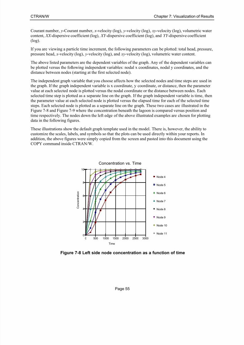
7/25/2019 Ctran Modeling
http://slidepdf.com/reader/full/ctran-modeling 63/101
CTRAN/W Chapter 7: Visualization of Results
Page 55
Courant number, y-Courant number, x-velocity (log), y-velocity (log), xy-velocity (log), volumetric water
content, XX -dispersive coefficient (log), XY -dispersive coefficient (log), and YY -dispersive coefficient
(log).
If you are viewing a particle time increment, the following parameters can be plotted: total head, pressure,
pressure head, x-velocity (log), y-velocity (log), and xy-velocity (log), volumetric water content.
The above listed parameters are the dependent variables of the graph. Any of the dependent variables can
be plotted versus the following independent variables: nodal x coordinates, nodal y coordinates, and the
distance between nodes (starting at the first selected node).
The independent graph variable that you choose affects how the selected nodes and time steps are used in
the graph. If the graph independent variable is x coordinate, y coordinate, or distance, then the parameter
value at each selected node is plotted versus the nodal coordinate or the distance between nodes. Each
selected time step is plotted as a separate line on the graph. If the graph independent variable is time, then
the parameter value at each selected node is plotted versus the elapsed time for each of the selected time
steps. Each selected node is plotted as a separate line on the graph. These two cases are illustrated in theFigure 7-8 and Figure 7-9 where the concentration beneath the lagoon is compared versus position and
time respectively. The nodes down the left edge of the above illustrated examples are chosen for plotting
data in the following figures.
These illustrations show the default graph template used in the model. There is, however, the ability to
customize the scales, labels, and symbols so that the plots can be used directly within your reports. In
addition, the above figures were simply copied from the screen and pasted into this document using the
COPY command inside CTRAN/W.
Figure 7-8 Left side node concentration as a function of time
Concentration vs. Time
Node 4
Node 5
Node 6
Node 7
Node 8
Node 9
Node 10
Node 11
C o n c e n t r a t i o n
Time
0
2
4
6
8
10
0 500 1000 1500 2000 2500 3000

7/25/2019 Ctran Modeling
http://slidepdf.com/reader/full/ctran-modeling 64/101
Chapter 7: Visualization of Results CTRAN/W
Page 56
Figure 7-9 Left side node concentration as a function of y coordinate for each time
7.5 “None” values
In GeoStudio, an attempt is made to distinguish between data values that have a true value of zero, andthose that are missing. A missing value is labeled as “none” in a data list or is not printed to file when
you save the data for export or pasting into another program such as Excel. A missing value is simply a
data type that is not relevant to the current set of analysis parameters.
“None” or missing values, are simply a way for GeoStudio to not erroneously report data values as zero
(which has meaning) when they really just do not exist. Consider the following graph generated by
GeoStudio of pore-water pressures in a soil as it is placed during a construction sequence. At the 0
second time, the soil surface is at 10m. At 10 seconds, 2 meters of more soil is added. At 8010 seconds,
another 2 meters is added. Notice that for the two added lifts of soil, the pressure values are not graphedas zero prior to their placement time. The data is “missing” in the program so is not reported or graphed.
Figure 7-10 Graph showing how missing data is excluded and not printed as zero
Concentration vs. Y
0.0000e+000
2.5000e+002
5.0000e+002
7.5000e+0021.0000e+003
1.2500e+003
1.5000e+003
1.7500e+003
2.0000e+003
2.2500e+003
2.5000e+003
2.7500e+003
Y
Concentration
2
4
6
8
10
0 2 4 6 8 10
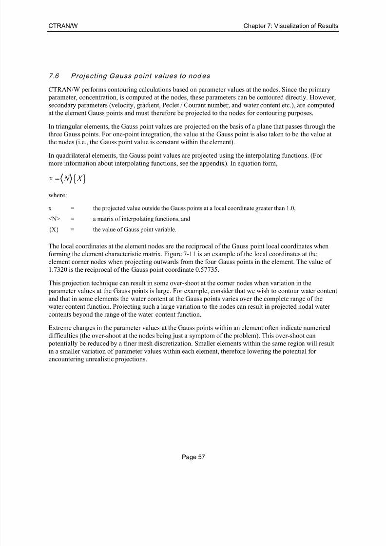
7/25/2019 Ctran Modeling
http://slidepdf.com/reader/full/ctran-modeling 65/101
CTRAN/W Chapter 7: Visualization of Results
Page 57
7.6 Project ing Gauss point values to nod es
CTRAN/W performs contouring calculations based on parameter values at the nodes. Since the primary
parameter, concentration, is computed at the nodes, these parameters can be contoured directly. However,
secondary parameters (velocity, gradient, Peclet / Courant number, and water content etc.), are computed
at the element Gauss points and must therefore be projected to the nodes for contouring purposes.
In triangular elements, the Gauss point values are projected on the basis of a plane that passes through the
three Gauss points. For one-point integration, the value at the Gauss point is also taken to be the value at
the nodes (i.e., the Gauss point value is constant within the element).
In quadrilateral elements, the Gauss point values are projected using the interpolating functions. (For
more information about interpolating functions, see the appendix). In equation form,
{ } N X =
where:
x = the projected value outside the Gauss points at a local coordinate greater than 1.0,
<N> = a matrix of interpolating functions, and
{X} = the value of Gauss point variable.
The local coordinates at the element nodes are the reciprocal of the Gauss point local coordinates when
forming the element characteristic matrix. Figure 7-11 is an example of the local coordinates at the
element corner nodes when projecting outwards from the four Gauss points in the element. The value of
1.7320 is the reciprocal of the Gauss point coordinate 0.57735.
This projection technique can result in some over-shoot at the corner nodes when variation in the parameter values at the Gauss points is large. For example, consider that we wish to contour water content
and that in some elements the water content at the Gauss points varies over the complete range of the
water content function. Projecting such a large variation to the nodes can result in projected nodal water
contents beyond the range of the water content function.
Extreme changes in the parameter values at the Gauss points within an element often indicate numerical
difficulties (the over-shoot at the nodes being just a symptom of the problem). This over-shoot can
potentially be reduced by a finer mesh discretization. Smaller elements within the same region will result
in a smaller variation of parameter values within each element, therefore lowering the potential for
encountering unrealistic projections.

7/25/2019 Ctran Modeling
http://slidepdf.com/reader/full/ctran-modeling 66/101
Chapter 7: Visualization of Results CTRAN/W
Page 58
Figure 7-11 Local coordinates at the corner nodes of an element with four integrationpoints
7.7 Contours
The power of using advanced graphical interfaces with finite element analysis is that the computer canquickly convert thousands of pieces of data into meaningful pictures. In the section above we introduced
isotherms. We can use a picture of the isochlors to tell us something about what is going on in the soil. In
particular, if we consider how close adjacent isochlors are to each other, we are in effect, considering how
steep the concentration gradient is. If we recall that the amount of mass flow is equal to the concentration
gradient multiplied by the dispersion coefficient, we then have a fast and clear picture of where the areas
of high mass flow are in the domain we have modeled.
CTRAN/W is a powerful tool in that it will let you contour many different parameters such as
concentration, Courant number, Peclet number, pressure, gradients, mass fluxes, water contents and more.
Figure 7-12 is a contour of the X direction Courant number values for the isochlors illustrated above. We
know that for an advection-dispersion type analysis, we want the Courant number to remain low. This
figure shows us that it ranges between 0.05 and perhaps 0.5, which is acceptable. If this contour were to
have shown us areas of high Courant or Peclet value, we would have an idea of what to adjust in order to
obtain a better solution. Perhaps the mesh would need to be finer in one location or the time steps smaller.
Figure 7-12 CTRAN/W computed X direction Courant numbers
C = 10
Free Exit
0 . 0
5
0 .0 5
0 . 1
0 . 1 5
0 .2 5
0 . 2 5
0. 3 5

7/25/2019 Ctran Modeling
http://slidepdf.com/reader/full/ctran-modeling 67/101
CTRAN/W Chapter 7: Visualization of Results
Page 59
7.8 Water f low vectors and f low paths
Water flow vectors and flow paths are described in detail in the SEEP/W and VADOSE/W engineering
books.
7.9 Anim at ion in GeoStudio
Movie files (*.avi) can be created in GeoStudio to illustrate a physical process in a transient analysis. The
first step in creating a movie is to define the contours and specify any View Preferences that need to be
visible (e.g. flux vectors or the displaced mesh). The View Animation command is selected and the time
steps and viewing area are defined. After saving the movie file to the appropriate location, GeoStudio
joins together all of the individual images for each time step, creating a seamless animated movie.
7.10 Flux sectio ns
CTRAN/W has the ability to compute the instantaneous flux across a user-defined section for either asteady-state or transient analysis. The view preference command can be used to modify the flux type that
is displayed on the flux section. View Preferences allows you to display total, advective, dispersive,
stored, or decayed flux on the drawing. The stored flux is the rate at which mass is stored in an element. Anegative stored mass means that mass is accumulating in an element (i.e., the total mass flow across the
section is decreasing due to adsorption). A positive stored flux means that mass is being released from the
element, thereby increasing the rate of mass flow across the section.
Flux sect ion theory
Details of the flux section calculations are given in the Theory chapter.
Flux sect ion appl icat ion
Flux sections can be used in many ways, because they can be drawn any place across which you want to
know the flux. You may want to check if an influx is equal to an out-flux such as illustrated in Figure7-13. In this case, the values are NOT the same which is to be expected because the problem is a transient
analysis and there is a change in the amount of mass storage over time.

7/25/2019 Ctran Modeling
http://slidepdf.com/reader/full/ctran-modeling 68/101
Chapter 7: Visualization of Results CTRAN/W
Page 60
Figure 7-13 Flux section used to check balance of mass inflow and outflow
Flux sections do not have to be drawn as single straight lines. They can be made of continuous attached
segments as illustrated in the figure above. When a multiple segmented flux section is drawn, the value of
flux reported for the section applies to the entire section, not any individual segment.
The key point to note when defining a flux section is to make the flux section cross the sides of the
elements and not the nodes of the elements. Also, if you want to check the flux around a closed loop as
illustrated for the SEEP/W seepage drain nodes in Figure 7-14, make sure the end of the flux section
crosses over the tail of the first segment of the flux section.
Two words of caution: flux sections MUST be defined before you solve the problem, because the
program needs to calculate the values during the solution sequence, not afterward. In addition, all flux
values are reported as positive, which means direction is not taken into account. This is required because
the sign of the flux value will depend on which way you draw the section. To avoid any misinterpretation,
all flux section values are reported as positive, and then you can plot flux vectors in order to determine the
direction of flow, if it is not obvious based on your problem definition.
C = 10
Free Exit
3 . 3 0 3 5 e - 0 0 2
1 . 6
6 8 9
e -
0 0 1
metres
0 1 2 3 4 5 6 7 8 9 10 11 12 13 14 15 16 17 18 19 20 21 22 230
1
2
3
4
5
6
7
8
9
10
11
12
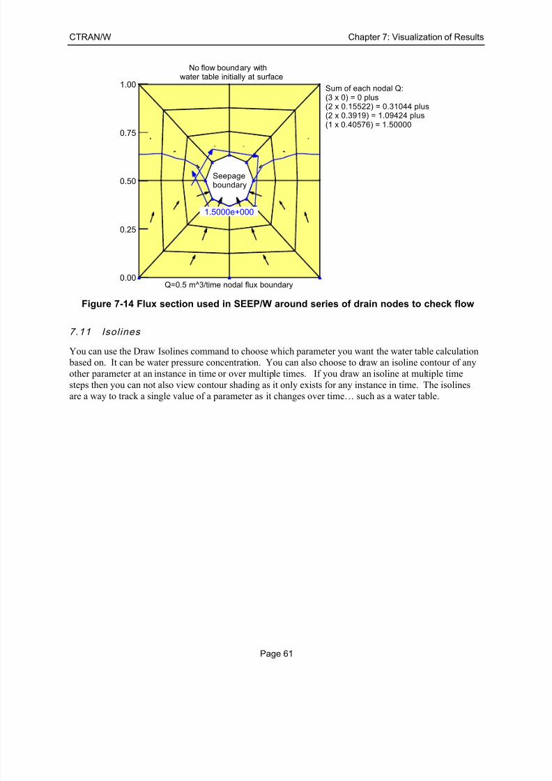
7/25/2019 Ctran Modeling
http://slidepdf.com/reader/full/ctran-modeling 69/101
CTRAN/W Chapter 7: Visualization of Results
Page 61
Figure 7-14 Flux section used in SEEP/W around series of drain nodes to check flow
7.11 Isol ines
You can use the Draw Isolines command to choose which parameter you want the water table calculation
based on. It can be water pressure concentration. You can also choose to draw an isoline contour of any
other parameter at an instance in time or over multiple times. If you draw an isoline at multiple time
steps then you can not also view contour shading as it only exists for any instance in time. The isolines
are a way to track a single value of a parameter as it changes over time… such as a water table.
Sum of each nodal Q:(3 x 0) = 0 plus(2 x 0.15522) = 0.31044 plus(2 x 0.3919) = 1.09424 plus(1 x 0.40576) = 1.50000
No flow boundary withwater table initially at surface
Seepageboundary
Q=0.5 m^3/time nodal flux boundary
1.5000e+000
0.00
0.25
0.50
0.75
1.00

7/25/2019 Ctran Modeling
http://slidepdf.com/reader/full/ctran-modeling 70/101
Chapter 7: Visualization of Results CTRAN/W
Page 62
.
7/25/2019 Ctran Modeling
http://slidepdf.com/reader/full/ctran-modeling 71/101
CTRAN/W Chapter 8: Modeling tips and tricks
Page 63
8 Modeling Tips and Tricks
8.1 Introduct ion
This chapter contains many useful hints about using the software and understanding what it does. READ
THIS CHAPTER!
CTRAN/W is a powerful analytical tool, but it will only provide valid solutions if the boundary
conditions, material properties, and time sequence are appropriately defined. It is your responsibility to
properly define the problem parameters and ensure that the results produced are valid and reasonable.
This chapter presents some general modeling guidelines. The information presented is not an exhaustive
statement on the "how-to" of modeling a contaminant transport problem. Instead, it is intended to provide
suggestions on how you might model various conditions, as well as to outline the implications of certain
modeling specifications.
There have been many occasions where GEO-SLOPE has been contacted by clients with questions about
how the model behaves in response to changes in various parameters. If we do not know the answer, we
conduct a numerical experiment to test what will happen. The first few sections of this chapter illustrate afew common examples of numerical experiments. You are strongly encouraged to learn why these types
of simple tests are so powerful in testing how the program computes results BUT ALSO in enhancing
your understanding of how the physical mechanisms of flow through porous medium occurs.
A numerical experiment is carried out by making a very simple finite element problem. It is useful to use
a mesh that is one distance unit wide and one distance unit high. This makes hand calculating flux values
very simple and they can easily be checked against the computed flux values. The following discussion
illustrates how some simple numerical experiments have been carried out to test some simple, yet valid,
questions.
When setting up these experiments, it is a good idea to input simple soil property functions. In most cases,
two data points are sufficient to define the conductivity and storage function. Just as a reminder, give bothfunctions some slope – don’t make them horizontal!
8.2 Model ing prog ression
Modeling the movement of contaminants through soil is a complex type of analysis. As discussed in the
Theory Chapter, the contaminant transport process is not only governed by water movement, it is also
influenced by dispersion, molecular diffusion, adsorption, and radioactive decay. With so many factors
involved, it can be confusing and difficult to resolve the contribution of each component in the transport
process.
An important rule to follow in contaminant transport modeling is to progress from the simple to the
complex. It is good practice to initially define a simplified version of the problem and then addcomplexity in stages. Moving from the simple to the complex makes it easier to pinpoint difficulties with
the model when the results of the analysis are unrealistic.
For example, begin by analyzing a homogeneous problem with no adsorption and no decay. Then add
adsorption, decay, and other materials to the analysis in separate stages. This incremental approach not
only helps to evaluate the results but also provides information on the effect of the various parameters.
Determining what causes unrealistic results can be difficult if all of the possible complexities are included
at the start of the problem analysis.
7/25/2019 Ctran Modeling
http://slidepdf.com/reader/full/ctran-modeling 72/101
Chapter 8: Modeling tips and tricks CTRAN/W
Page 64
For complex transport problems that may involve multiple sources and exit boundaries, it is useful to first
do a particle tracking analysis before doing the advection-dispersion transport modeling. Particle tracking
has the advantage of providing an approximate solution to the transport problem quickly with minimum
input requirements. Although only the advection process (water movement) is considered in particle
tracking, the solution does provide a clear picture of the approximate contaminant plume.
8.3 Problem engineering uni ts
Any system of units can be used for a contaminant transport analysis; the only requirement is that you
must be consistent with the units throughout both the CTRAN/W and the corresponding seepage analysis.
Fundamentally, you must select the units for length (geometry), time, and force. Once you have selected
units for these parameters, all other units must be consistent. Table 8-1 and Table 8-2 present some
typical sets of consistent units.

7/25/2019 Ctran Modeling
http://slidepdf.com/reader/full/ctran-modeling 73/101
CTRAN/W Chapter 8: Modeling tips and tricks
Page 65
Table 8-1 Consistent set of SI units
Parameter Symbol Units
Length L m
Time t s
Force F kN
Mass M g
Pressure F/L2 kN/m
2
Unit Weight of Water F/L3 kN/m
3
Hydraulic Conductivity L/T m/s
Concentration M/L3 g/m
3
Diffusion Coefficient L2 /T m
2/s
αL and αT (dispersivity) L m
Decay Half-Life T sec
S (adsorption) M/M g/g
Density M/L3 g/m
3
Mass Flux M/T g/s
Table 8-2 Consistent set of imperial units
Parameter Symbol Units
Length L ft
Time t hr
Force F lbf
Mass M lb
Pressure F/L2 psf
Unit Weight of Water F/L3 pcf
Hydraulic Conductivity L/T ft/hr
Concentration M/L3 lb/ft
3
Diffusion Coefficient L2 /T ft
2/hr
αL and αT (dispersivity) L ft
Decay Half-Life T hr
S (adsorption) M/M lb/lb
Density M/L3 lb/ft
3
Mass Flux M/T lb/hr
The units of time are established once you select the units for hydraulic conductivity. The units of
pressure are established once you select the unit weight of water. Generally, all units are defined by
selecting the units of length for the problem geometry, units for hydraulic conductivity, and the units for
the unit weight of water.
Concentration is often reported in units of milligrams per liter (One milligram per liter (mg/l) is
equivalent to one part per million (ppm) and is also equivalent to one gram per cubic metre (g/m3). In
equation form: mg/l = ppm = g/m3.
Therefore, concentrations reported in mg/l or ppm can be conveniently used in a CTRAN/W analysis
provided mass is defined in grams (g) and length is defined in meters (m).

7/25/2019 Ctran Modeling
http://slidepdf.com/reader/full/ctran-modeling 74/101
Chapter 8: Modeling tips and tricks CTRAN/W
Page 66
In summary, the key requirement is that the system of units must be consistent.
8.4 Fracture f low simu lat ion
CTRAN/W can be used to analyze contaminant flow through fractures by modifying the definitions for
volumetric water content ( )Θ
, adsorption (S ), and the dry bulk density ( )d ρ . For fracture flow, these parameters are defined as:
Volume of Fractures =
Total VolumeΘ
Mass of Solute Adsorbed on the Fractures =
Unite Area of the FracturesS
Area of the Fracture Planes =
Total Volumed
ρ
The adsorption terms in the finite element equation involve ( )d multiplied by (S). Multiplying thesetwo variables together results in units of mass adsorbed on the fractures per unit volume. The area of the
fracture planes vanishes as far as the units are concerned.
8.5 Flux sect ion locat ion
Question: Does the location of a flux section within an element have any influence on the computed flux
value?
Answer: No. The flux section value will be the same regardless of whether the section is drawn near the
element edge or element middle. Figure 8-1 shows this to be the case and it is true for a transient and
steady state solution.
Figure 8-1 Test to check flux section locations
2.6869e+002
2.6869e+002
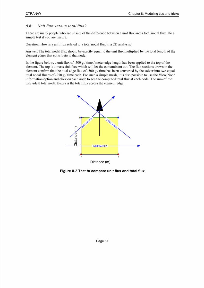
7/25/2019 Ctran Modeling
http://slidepdf.com/reader/full/ctran-modeling 75/101
CTRAN/W Chapter 8: Modeling tips and tricks
Page 67
8.6 Uni t f lux versus total f lux?
There are many people who are unsure of the difference between a unit flux and a total nodal flux. Do a
simple test if you are unsure.
Question: How is a unit flux related to a total nodal flux in a 2D analysis?
Answer: The total nodal flux should be exactly equal to the unit flux multiplied by the total length of the
element edges that contribute to that node.
In the figure below, a unit flux of -500 g / time / meter edge length has been applied to the top of the
element. The top is a mass sink face which will let the contaminant out. The flux sections drawn in the
element confirm that the total edge flux of -500 g / time has been converted by the solver into two equal
total nodal fluxes of -250 g / time each. For such a simple mesh, it is also possible to use the View Nodeinformation option and click on each node to see the computed total flux at each node. The sum of the
individual total nodal fluxes is the total flux across the element edge.
Figure 8-2 Test to compare unit flux and total flux
5.0000e+002
2 . 5 0
0 0 e +
0 0 2 2 .5 0 0 0 e + 0 0 2
Distance (m)
5 6
D i s t a n c e ( m )
0
1

7/25/2019 Ctran Modeling
http://slidepdf.com/reader/full/ctran-modeling 76/101

7/25/2019 Ctran Modeling
http://slidepdf.com/reader/full/ctran-modeling 77/101
CTRAN/W Chapter 9: Illustrative Examples
Page 69
9 Illustrative Examples
A variety of verification and illustrative examples has been developed and are available with the software.
These examples can be useful for learning how to model various problems, particularly in the selection
and application of boundary conditions. Each example comes with a PDF document that provides
explanations on the problem setup, comments on modeling techniques and a commentary on interpretingthe results. Verification examples are discussed in terms of closed-form solutions, published information
and/or laboratory measurements.
All of the examples can be downloaded and installed from GEO-SLOPE’s web site (www.geo-
slope.com). Once installed, it is possible to search for a particular type of analysis on the GeoStudio
desktop. Conversely, the search feature is available directly on the website. It should be noted that a
product-specific search is possible (e.g. search for TEMP/W or SIGMA/W).
The GeoStudio example files can be reviewed using the free GeoStudio Viewer license.

7/25/2019 Ctran Modeling
http://slidepdf.com/reader/full/ctran-modeling 78/101
7/25/2019 Ctran Modeling
http://slidepdf.com/reader/full/ctran-modeling 79/101
CTRAN/W Chapter 10: Theory
Page 71
10 Theory
This chapter presents the methods, equations, procedures, and techniques used in the CTRAN/W
formulation. It is of value to be familiar with this information in order to use the software. An
understanding of these concepts will be of great benefit in applying the software, resolving difficulties,
and judging the acceptability of the results.
10.1 Flow velocity
SEEP/W and VADOSE/W compute the specific discharge or D’Arcy velocity. The specific discharge is
the total flux Q divided by the full cross-sectional area (voids and solids alike).
The actual cross-sectional area available for the water is less than the full area, due to the presence of the
solids. Consequently, the actual rate of movement of the water is higher than the D’Arcy velocity. By
definition, the porosity is the volume of voids divided by the total volume. The cross-sectional area
available for the water flow is the porosity times the total cross-sectional area.
Therefore the average linear velocity of the pore fluid is: (see Freeze and Cherry, 1979)
=Q
vn A
or,
=U
vn
where:
U = specific discharge, or D’arcian velocity, and
n = porosity.
Under saturated conditions, the volumetric water content ( )Θ is equal to the porosity. The average linear
velocity then is also equal to:
=U
vΘ
CTRAN/W is formulated on the assumption that the average linear velocity can be related to the
volumetric water content for both saturated and unsaturated conditions. SEEP/W, being a
saturated/unsaturated flow model, computes the volumetric water content. The SEEP/W specific
discharge, (D’Arcy velocity), divided by the SEEP/W volumetric water content is taken in the CTRAN/W
formulation as the average linear velocity.
10.2 Governing equat ions
The governing equation for contaminant transport is generally known as the transport equation or the
advection-dispersion equation.
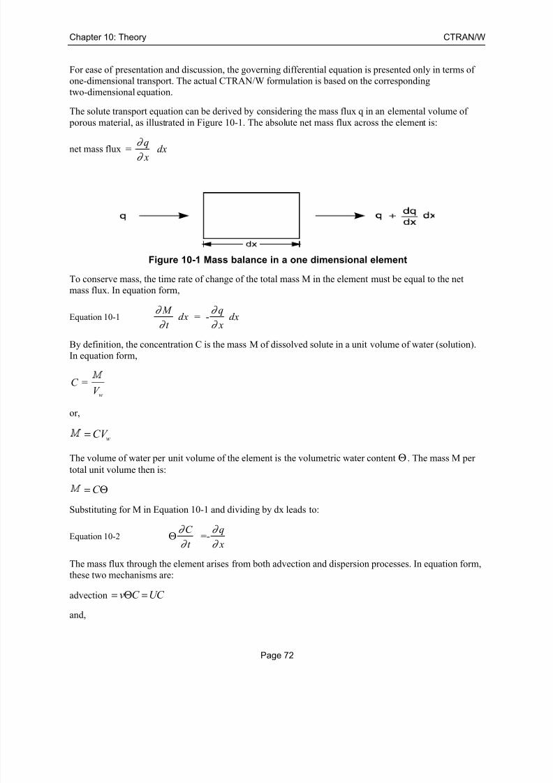
7/25/2019 Ctran Modeling
http://slidepdf.com/reader/full/ctran-modeling 80/101
Chapter 10: Theory CTRAN/W
Page 72
For ease of presentation and discussion, the governing differential equation is presented only in terms of
one-dimensional transport. The actual CTRAN/W formulation is based on the corresponding
two-dimensional equation.
The solute transport equation can be derived by considering the mass flux q in an elemental volume of
porous material, as illustrated in Figure 10-1. The absolute net mass flux across the element is:
net mass flux =q
dx x
∂
∂
Figure 10-1 Mass balance in a one dimensional element
To conserve mass, the time rate of change of the total mass M in the element must be equal to the net
mass flux. In equation form,
Equation 10-1 = - M q
dx dxt x
∂ ∂
∂ ∂
By definition, the concentration C is the mass M of dissolved solute in a unit volume of water (solution).
In equation form,
=w
C V
or,
wCV =
The volume of water per unit volume of the element is the volumetric water content Θ . The mass M per
total unit volume then is:
C = Θ
Substituting for M in Equation 10-1 and dividing by dx leads to:
Equation 10-2 =-C q
t x
∂ ∂
∂ ∂ Θ
The mass flux through the element arises from both advection and dispersion processes. In equation form,
these two mechanisms are:
advection v C UC = Θ =
and,

7/25/2019 Ctran Modeling
http://slidepdf.com/reader/full/ctran-modeling 81/101
CTRAN/W Chapter 10: Theory
Page 73
dispersionC
D∂
∂ = −Θ
where:
ν = average linear velocity,
Θ = volumetric water content,
C = concentration,
D = hydrodynamic dispersion coefficient, and
U = D’Arcy velocity (specific discharge).
The negative sign in the dispersion term indicates that the direction of the mass flow is from a high
concentration to a low concentration (that is, a negative gradient). Substituting the previous two terms
into Equation 10-2 leads to the basic transport equation:
Equation 10-32
2
= - - +C C
D U C
t x xC C
D U x
∂ ∂ ∂
∂ ∂ ∂ ∂ ∂
∂ ∂
Θ Θ
= Θ −
This equation can be divided by Θ , which leads to:
2
2 = -
C C C D v
t x x
∂ ∂ ∂
∂ ∂ ∂
where v is the average linear velocity. This is the form of the equation often seen in publications. (Freeze
and Cherry, 1979). CTRAN/W uses the more general form as shown in Equation 10-3.
The hydrodynamic dispersion coefficient D is related to the dispersivity, average linear velocity anddiffusion coefficient D* by:
* D v Dα = +
For further discussion regarding this coefficient, refer to the section on the Hydrodynamic Dispersion
Matrix later in this chapter.
Equation 10-3 represents the basic transport of a non-reactive and non-radioactive substance; that is, there
is no loss of mass due to adsorption or radioactive decay. For general formulation, the loss of mass due to
adsorption and radioactive decay must be added to the transport equation.
For the transport of a radioactive substance, mass may be lost during the transport process due to
radioactive decay of ions in the pore fluid and decay of ions attached to the soil particles. The reducedconcentration resulting from radioactive decay, in terms of the initial concentration, is:
Equation 10-4 0
t C C e λ −=
where t is the elapsed time and λ is the decay coefficient. The decay coefficient λ can be related to the
half-life T of a decaying material. By definition, the half-life T is the elapsed time when the concentration
of C/C0 = 1/2. Therefore,

7/25/2019 Ctran Modeling
http://slidepdf.com/reader/full/ctran-modeling 82/101
Chapter 10: Theory CTRAN/W
Page 74
-
0
1 = =
2
T C e
C
λ
which can also be written as:
ln 2 0.693 = =T T λ
Differentiating Equation 2-1 with respect to time leads to:
= -C
C t
∂ λ
∂
The amount of radioactive mass in the pore-water Mw in an elemental unit volume is C Θ , (see above),
or:
0
t
w C C e λ −= Θ = Θ
The adsorption S is the amount of mass attached to the soil particles divided by the mass of the solids. In
equation form,
mass of solute attached to the solids=
mass of the solidsS
The mass per unit volume of the soil (solid) particles can be defined in terms of the bulk (dry) mass
density d ρ of the soil. The parameter S is then defined as:
= s
d
S
or,
Equation 10-5 d S ρ =
where Ms is the amount of mass attached to a unit mass of soil particles.
In terms of radioactive decay,
0
t
s d d S S e λ ρ ρ −= =
Therefore, the total radioactive mass M in both the fluid and solid phases is:
0 0
w s
t t
d
M M M
C e S eλ λ ρ − −
= +
= Θ +
The rate of change of mass due to decay is then:
M = - C - S
t d
∂ λ λ ρ
∂ Θ

7/25/2019 Ctran Modeling
http://slidepdf.com/reader/full/ctran-modeling 83/101
CTRAN/W Chapter 10: Theory
Page 75
The transport equation (Equation 10-3) can now be modified to include radioactive decay. The result is:
Equation 10-6
2
2 = - - -
d
C C C D U C S
t x x
∂ ∂ ∂ λ λ ρ
∂ ∂ ∂ Θ Θ Θ
For the transport of a reactive substance, the movement of the mass is also affected by the adsorption of
the solute by the soil particles. As discussed above, the amount of mass adsorbed can be defined in termsof the mass density of the soil particles. From Equation 10-5, the adsorbed mass Ms is:
s d S ρ =
The rate of change of the adsorbed mass is:
= sd
M S
t t
∂ ∂ ρ
∂ ∂
The adsorption S is a function of concentration C. Experimental results are usually plotted as S vs. C, as
shown in Figure 10-2. The slope of the S vs. C relationship is /S C ∂ ∂ . In the case of a linear
relationship, the slope is usually referred to as the distribution coefficient Kd. The previous equation canthen be written as:
= sd
M S C
t C t
∂ ∂ ∂ ρ
∂ ∂ ∂
Adding the adsorption term to Equation 10-6 gives the following governing differential equation used in
CTRAN/W:
2
2 + = - - -
d d
C S C C C D U C S
t C t x x
∂ ∂ ∂ ∂ ∂ ρ λ λ ρ
∂ ∂ ∂ ∂ ∂ Θ Θ Θ
or,
Equation 10-7
2
2+ = - - -d d
S C C C D U C S
C t x x
∂ ∂ ∂ ∂ ρ λ λ ρ
∂ ∂ ∂ ∂
Θ Θ Θ
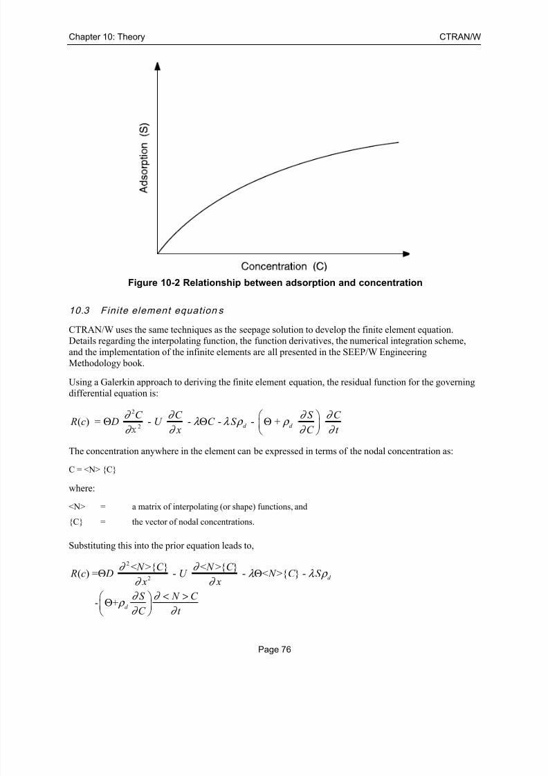
7/25/2019 Ctran Modeling
http://slidepdf.com/reader/full/ctran-modeling 84/101
Chapter 10: Theory CTRAN/W
Page 76
Figure 10-2 Relationship between adsorption and concentration
10.3 Finite element equation s
CTRAN/W uses the same techniques as the seepage solution to develop the finite element equation.
Details regarding the interpolating function, the function derivatives, the numerical integration scheme,
and the implementation of the infinite elements are all presented in the SEEP/W Engineering
Methodology book.
Using a Galerkin approach to deriving the finite element equation, the residual function for the governing
differential equation is:
2
2( ) = - - - - +d d
C C S C R c D U C S
x C t
∂ ∂ ∂ ∂ λ λ ρ ρ
∂ ∂ ∂ ∂
Θ Θ Θ
The concentration anywhere in the element can be expressed in terms of the nodal concentration as:
C = <N> {C}
where:
<N> = a matrix of interpolating (or shape) functions, and
{C} = the vector of nodal concentrations.
Substituting this into the prior equation leads to,
2
2
< >{ } < >{ }( ) = - - < >{ } -
- +
d
d
N C N C R c D U N C S
x x
S N C
C t
∂ ∂ λ λ ρ
∂ ∂
∂ ∂ ρ
∂ ∂
Θ Θ
< > Θ

7/25/2019 Ctran Modeling
http://slidepdf.com/reader/full/ctran-modeling 85/101
CTRAN/W Chapter 10: Theory
Page 77
The residual can now be multiplied by a weighting function <N>T, then integrated over the volume, and
then set to zero in order to minimize the residual. The resulting equation is:
2
2
< >0 = < > { }T
v
N D N dv C
x
∂
∂ Θ
< >< > { }T
v
N U N dv C x
∂ ∂
−
< > < > { }T
v N N dv C λ − Θ
< >T
d v
S N dvλρ −
+ < > < > { },T
d t v
S N N dv C
C
∂ ρ
∂
− Θ
Applying Green’s theorem, the first term can be integrated by parts to give:
2
2v s
<N> <N>D < > dv = D < > ds
x
<N> <N>
T T
T
v
N N n
D dv x
∂ ∂
∂ ∂
∂ ∂
∂ ∂
Θ Θ
− Θ
where n is a direction unit vector normal to the surface.
Substituting this into the first term in the previous equation results in:
< > < > < >0 = < > { } - { }
T T
s v
N N N D N ds C D dv C
n x x
∂ ∂ ∂
∂ ∂ ∂ Θ Θ
< > < > { }T
v
N U N dv C
x
∂
∂ −
< > < > { }T
v N N dv C λ − Θ
< >T
d v
S N dvλρ −
+ < > < > { },T
d t v
S N N dv C
C
∂ ρ
∂
− Θ
The derivatives of the interpolating functions are designated as the gradient matrix [B]. Substituting [B]
for the gradient terms and rearranging the terms leads to:
Equation 10-8 [ ] [ ][ ] { }T
v B D B dv C Θ (Term 1)
< > [ ][ ] { }T
v N U B dv C + (Term 2)

7/25/2019 Ctran Modeling
http://slidepdf.com/reader/full/ctran-modeling 86/101
Chapter 10: Theory CTRAN/W
Page 78
< > < > { }T
v N N dv C λ + Θ (Term 3)
+ < > < > { },T
d t v
S N N dv C
C
∂ ρ
∂
+ Θ
(Term 4)
< > < > { }T
s N D N ds C n
∂ ∂
= Θ (Term 5)
< >T
d v
S N dvλρ − (Term 6)
The surface integral on the right hand side of Term 5 represents the dispersive mass flux across the
boundary, and is the natural boundary condition. However, there may also be advective mass flux across
the boundary which will be equal to the specific discharge at the boundary Ub times the concentration.
A more practical boundary condition is the specification of the total mass flux across the boundary (i.e.,
the Cauchy type or the Third type boundary condition). This total mass flux q will be the sum of the
dispersive flux and the advective flux across the boundary. In equation form,
= +b
C q D U C
n
∂
∂ Θ
Expressing the element concentration C in terms of the nodal concentration {C} and the shape function
<N>: (See above)
Equation 10-9< >{ }
= + < >{ }b
N C q D U N C
n
∂
∂ Θ
The term,< >{ } N C
n
∂
∂ signifies that the flow is normal (n) to the boundary.
Equation 10-7 can be rearranged as:
< >{ } = - < >{ }
b
N C D q U N C
n
∂
∂ Θ
Therefore, Term 5 of Equation 10-6 can be expressed as:
< > < > { } = < >T T
s s
N D N ds C q N ds
n
∂
∂ Θ
- < > < > { }T
b s
U N N ds C
Substituting this in Equation 10-6 leads to the general finite element equation used in the CTRAN/Wformulation:
Equation 10-10 [ ] [ ][ ] { }T
v B D B dv C Θ (Term 1)
< > [ ][ ] { }T
v N U B dv C + (Term 2)
7/25/2019 Ctran Modeling
http://slidepdf.com/reader/full/ctran-modeling 87/101
CTRAN/W Chapter 10: Theory
Page 79
< > < > { }T
v N N dv C λ + Θ (Term 3)
+ < > < > { },T
d t v
S N N dv C
C
∂ ρ
∂
+ Θ
(Term 4)
< > < > { }T
b s U N N ds C +
(Term 5)
< >T
sq N ds= (Term 6)
< >T
d v
S N dvλρ − (Term 7)
In abbreviated form, the finite element equation can be written as:
[ ]{ } [ ]{ } { }{ }{ } { }{ }1 2 1 2, , K C K C t Q K C K C t Q+ = + =
where:
{K1} = the element characteristic matrix,
= the Dispersive Mass Flux (Term 1),
+ the Advective Mass Flux (Term 2),
+ the fluid phase Decayed Mass Flux (Term 3),
+ the boundary Advective Mass Flux (Term 5),
{K2} = the element capacitance (storage) matrix,
= the Stored Mass Flux (Term 4),
{Q} = the mass flux entering or leaving the element,= the specified Nodal Total Mass Flux (Term 6), and
+ the solid phase Decayed Mass Flux (Term 7).
10.4 Temporal integr ation
The finite element solution for the transport equation is a function of time as indicated by the {C},t term
in the finite element equation. The time integration can be performed by a finite difference approximation
scheme. CTRAN/W uses the following general equation for the time integration:
[ ] [ ]( ){ } { } ( ) { }( )
[ ] ( ) [ ]( ){ }
1 2 1 1 0
2 1 0
1
1
t K K C t Q t Q
K t K C
ω ω ω
ω
∆ + = ∆ + − ∆
+ − − ∆
where:
t ∆ = time increment,
ω = a ratio between 0 and 1,
7/25/2019 Ctran Modeling
http://slidepdf.com/reader/full/ctran-modeling 88/101
Chapter 10: Theory CTRAN/W
Page 80
{C1} = nodal concentration at end of time increment,
{C0} = nodal concentration at start of time increment,
{Q1} = nodal mass flux at end of time increment,
{Q0} = nodal mass flux at start of time increment,
{K1} = element characteristic matrix, and
{K2} = element capacitance (storage) matrix.
CTRAN/W allows you to select between the Backward Difference Approximation Method (BDA) with
ω being set to 1, and the Central Difference Approximation Method (CDA) with ω being set to 0.5. For
more information about which time integration method to use, see Backward or Central Difference Time
in the chapter on Numerical Issues.
As indicated by the above equation, in order to solve for the nodal concentration at the end of the time
increment, it is necessary to know the nodal concentration at the start of the time increment. Stated in
general, the initial conditions must be known for solving the transport equation.
When the initial conditions are not specified, CTRAN/W assumes the initial nodal concentration as zero.
10.5 Hydrod ynamic dispers ion matr ix
For one-dimensional flow, the hydrodynamic dispersion coefficient D is defined above as:
* D v Dα = +
where:
α = dispersivity (material property),
ν = D’arcian velocity divided by volumetric water content (U/Θ), and
D* = coefficient of molecular diffusion.
Dispersion in the direction of the water flow is usually higher than dispersion perpendicular to the flow
direction. Two dispersivity values are therefore required to define the spreading process. Dispersivities in
the flow directions are designated as the longitudinal dispersivity Lα and the transverse dispersivity T
α .
For two-dimensional flow, as used in the CTRAN/W formulation, the hydrodynamic dispersion
coefficient D can be defined in matrix form: (See Bear, 1979)
11 12
21 22
D D
D D
where:
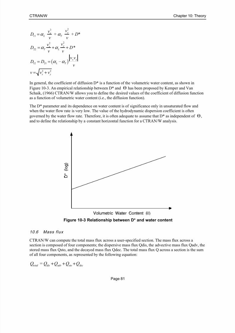
7/25/2019 Ctran Modeling
http://slidepdf.com/reader/full/ctran-modeling 89/101
CTRAN/W Chapter 10: Theory
Page 81
( )
22
11
22
22
12 21
2 2
+ + *
*
y x L T
y xT L
x y
L T
x y
vv D D
v v
vv D D
v v
v v D D
v
v v v
α α
α α
α α
=
= + +
= = −
= +
In general, the coefficient of diffusion D* is a function of the volumetric water content, as shown in
Figure 10-3. An empirical relationship between D* and Θ has been proposed by Kemper and Van
Schaik, (1966) CTRAN/W allows you to define the desired values of the coefficient of diffusion function
as a function of volumetric water content (i.e., the diffusion function).
The D* parameter and its dependence on water content is of significance only in unsaturated flow and
when the water flow rate is very low. The value of the hydrodynamic dispersion coefficient is often
governed by the water flow rate. Therefore, it is often adequate to assume that D* as independent of Θ ,and to define the relationship by a constant horizontal function for a CTRAN/W analysis.
Figure 10-3 Relationship between D* and water content
10.6 Mass flux
CTRAN/W can compute the total mass flux across a user-specified section. The mass flux across a
section is composed of four components; the dispersive mass flux Qdis, the advective mass flux Qadv, the
stored mass flux Qsto, and the decayed mass flux Qdec. The total mass flux Q across a section is the sum
of all four components, as represented by the following equation:
=total dis adv sto decQ Q Q Q Q+ + +

7/25/2019 Ctran Modeling
http://slidepdf.com/reader/full/ctran-modeling 90/101
Chapter 10: Theory CTRAN/W
Page 82
10.7 Dispers ive mass flux
The dispersive mass flux is computed in the same way as SEEP/W computes the water flux across a
section. For full details see the Theory chapter of the SEEP/W Engineering Methodology book.
As described in the SEEP/W book, consider a mesh with only one element
Figure 10-4 Illustration of mass flux section
The finite element equations of the dispersive mass flux term for one element can be expressed as
follows:
111 12 13 14 1
221 22 23 24 2
31 32 33 34 3 3
41 42 43 44 4 4
dis
dis
dis
dis
Qd d d d C
Qd d d d C
d d d d C Qd d d d C Q
=
The d coefficients in the above equation are a representation of the dispersion properties of the element.
Therefore, the dispersive mass flux from Node i to Node j is:
=dis ij ij i ji jQ d C d C −
The total dispersive mass flux through the flux section shown in Figure 10-4 is:
21 24 31 34=dis dis dis dis disQ Q Q Q Q+ + +
The imaginary flow lines from one side of the section to the other side are known as subsections.
CTRAN/W identifies all subsections across a user-defined flux section, computes the mass flux along
each subsection, and then sums the subsection values to obtain the total across the mass flux section.
10.8 Adv ect ive mass f lux
Both the advective mass flux term and the boundary advective mass flux term are used in the advective
mass flux calculations.

7/25/2019 Ctran Modeling
http://slidepdf.com/reader/full/ctran-modeling 91/101
CTRAN/W Chapter 10: Theory
Page 83
The finite element equations of the sum of the advective mass flux term and the boundary advective mass
flux term for one element can be expressed as follows:
111 12 13 14 1
221 22 23 24 2
31 32 33 34 3 3
41 42 43 44 4 4
adv
adv
adv
adv
Qa a a a C
Qa a a a C
a a a a C Q
a a a a C Q
=
The a coefficients in the above equation are a representation of the advective properties of the element.
Therefore, the advective mass flux from Node i to Node j is:
=adv ij ij i ji jQ a C a C −
The total advective mass flux through the flux section shown in Figure 10-4 is:
21 24 31 34=adv adv adv adv advQ Q Q Q Q+ + +
10.9 Stored mass flux
The stored mass flux is computed in the same way as SEEP/W computes the stored flux across a section.
The finite element equations of the stored mass flux term for one element can be expressed as follows:
111 12 13 14 1
221 22 23 24 2
31 32 33 34 3 3
41 42 43 44 4 4
1
sto
sto
sto
sto
Q s s s s C
Q s s s s C
s s s s C Qt
s s s s C Q
∆
∆ = ∆∆ ∆
where1 2, 3, ,C C C ∆ ∆ ∆ and 4C ∆ are the changes of concentration at the various nodes between the start
and the end of a time step. In general, the average change of concentration from Node i to Node j can be
expressed as:
=2
i j
ij
C C C
∆ + ∆∆
Therefore, the stored mass flux from Node i to Node j due to a change in storage is:
= s ij sto ij ij
C Q
t
∆
∆
The total stored mass flux through the flux section shown in Figure 10-4 is:
21 24 31 34= sto sto sto sto stoQ Q Q Q Q+ + +

7/25/2019 Ctran Modeling
http://slidepdf.com/reader/full/ctran-modeling 92/101
Chapter 10: Theory CTRAN/W
Page 84
10.10 Decayed mass flux
Both the fluid-phase decayed mass flux term and the solid-phase decayed mass flux term are used in the
decayed mass flux calculations.
For the fluid phase, the finite element equations of the decayed mass flux term for one element can be
expressed as follows:
111 12 13 14 1
221 22 23 24 2
31 32 33 34 3 3
41 42 43 44 4 4
fdec
fdec
fdec
fdec
Qdf df df df C
Qdf df df df C
df df df df C Q
df df df df C Q
=
The df coefficients in the above equation are a representation of the fluid phase decay properties of the
element. Therefore, the fluid phase decay mass flux calculated at the mid-point of Node i and Node j is:
( ) = 2
i j
fdec ij ij
C C Q df
+
As presented in the governing equation, the solid-phase decayed mass flux term is expressed in the form
of nodal mass flux to be subtracted from the specified nodal total mass flux term. The nodal mass flux due
to decay in the solid phase, Qsdec can be evaluated by the numerical integration of the solid phase
decayed mass flux term.
Therefore, the solid-phase decayed mass flux calculated at the mid-point of Node i and Node j is:
=2
sdec i sdec j
sdec ij
Q QQ
+
and, the total decayed mass flux at the mid-point of Node i and Node j is:
=dec ij fdec ij sdec ijQ Q Q+
The total decayed mass flux through the flux section shown in Figure 10-4 is:
21 24 31 34=dec dec dec dec decQ Q Q Q Q+ + +
10.11 Mass quanti ty calculat io n
CTRAN/W computes the mass quantity in both the fluid phase, Mf, and the solid phase, Ms of an element
by numerical integration of the following equations:
< > < > { }T
f v
N N dv C = Θ and
< > < > { }T
s d v
N N dv S ρ =
In performing the numerical integration of the above equations, CTRAN/W computes the concentration at
the Gauss point based on the nodal concentration and the interpolation function. The Gauss point
concentration is then used to compute the Gauss point adsorption S from the adsorption function. The
7/25/2019 Ctran Modeling
http://slidepdf.com/reader/full/ctran-modeling 93/101
CTRAN/W Chapter 10: Theory
Page 85
volumetric water content Θ at each Gauss point is obtained from the material file generated by SEEP/W
or VADOSE/W.
CTRAN/W computes the mass quantity at each Gauss point within an element. The Gauss point mass
quantity is calculated based on a weighted distribution of the element mass quantity to the Gauss points.
For the fluid phase, the distribution is weighted according to the product of *C Θ at each Gauss point.
Similarly, for the solid phase, the distribution is weighted according to the adsorption S at each Gauss point.
The mass quantity of each element is then summed to give the total mass quantity in the flow problem.
10.12 Ex it bo undaries
A unique solution to the transport equation requires the specification of boundary conditions around the
entire flow boundaries. In general, a boundary may be specified as a known concentration boundary or a
known mass flux boundary. In certain cases, however, neither the concentration nor the mass flux is
known, and, consequently, special considerations are required. This is the case at a boundary where mass
leaves the flow system (i.e., an exit boundary).
Two approaches are available for dealing with exit boundaries. One is to ignore the dispersive portion of
the mass flux and account only for the advective part of the flux (Qd=0). A second, more advanced
alternative is to account for both dispersive and advective mass flux at the exit boundary (Qd>0).
Equation 10-10 includes the term,
< > < > { }T
s
N D N ds C
n
∂
∂ Θ
This term represents the dispersive mass flux across a flow boundary and is the natural boundary term
derived as a result of the finite element formulation of the transport equation. The simplest option is to set
this natural boundary term to zero at the exit boundary (Qd=0). This approach is sometimes referred to as
a second type boundary condition. Setting the dispersive mass flux to zero has the effect of forcing theconcentration gradient to zero at the exit boundary.
Frind (1988), has proposed a method whereby the natural boundary term is solved and both the dispersive
and advective mass flux are accounted for at the exit boundary (Qd>0). This procedure results in what isreferred to as a free exit boundary. CTRAN/W uses this method in solving for the natural boundary term.
With a free exit boundary, the nodes along the exit boundary do not behave like ordinary boundary nodes.
Rather, they behave like all other internal nodes, making it possible to compute the concentration at these
nodes without assuming a certain concentration of mass flux to the nodes.
The free exit approach does not force the concentration gradient to zero, as with the second type
(i.e. zero dispersive mass flux) alternative. The effect of the two methods is illustrated in Figure 10-5.
Note that the solutions from the two methods are the same except near the exit boundary that is specifiedon the right hand side of the flow problem.
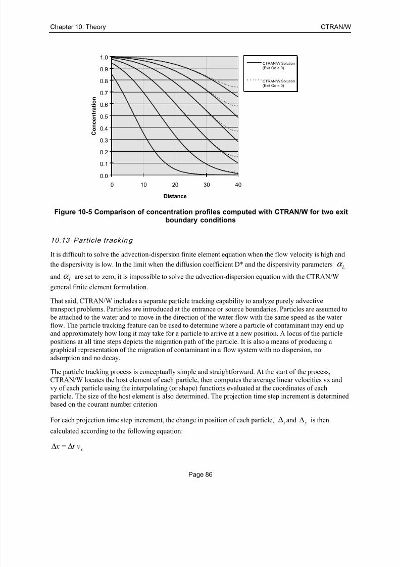
7/25/2019 Ctran Modeling
http://slidepdf.com/reader/full/ctran-modeling 94/101
Chapter 10: Theory CTRAN/W
Page 86
Figure 10-5 Comparison of concentration profiles computed with CTRAN/W for two exitboundary conditions
10.13 Part ic le trackin g
It is difficult to solve the advection-dispersion finite element equation when the flow velocity is high and
the dispersivity is low. In the limit when the diffusion coefficient D* and the dispersivity parameters Lα
and T α are set to zero, it is impossible to solve the advection-dispersion equation with the CTRAN/W
general finite element formulation.
That said, CTRAN/W includes a separate particle tracking capability to analyze purely advective
transport problems. Particles are introduced at the entrance or source boundaries. Particles are assumed to
be attached to the water and to move in the direction of the water flow with the same speed as the water
flow. The particle tracking feature can be used to determine where a particle of contaminant may end up
and approximately how long it may take for a particle to arrive at a new position. A locus of the particle
positions at all time steps depicts the migration path of the particle. It is also a means of producing a
graphical representation of the migration of contaminant in a flow system with no dispersion, no
adsorption and no decay.
The particle tracking process is conceptually simple and straightforward. At the start of the process,
CTRAN/W locates the host element of each particle, then computes the average linear velocities vx and
vy of each particle using the interpolating (or shape) functions evaluated at the coordinates of each
particle. The size of the host element is also determined. The projection time step increment is determined
based on the courant number criterion
For each projection time step increment, the change in position of each particle, x∆ and y∆ is then
calculated according to the following equation:
= x x t v∆ ∆
0.0
0.1
0.2
0.3
0.4
0.5
0.6
0.7
0.8
0.9
1.0
0 10 20 30 40
Distance
C o n c e n t r a t i o n
CTRAN/W Solution
(Exit Qd > 0)
CTRAN/W Solution(Exit Qd = 0)
7/25/2019 Ctran Modeling
http://slidepdf.com/reader/full/ctran-modeling 95/101
CTRAN/W Chapter 10: Theory
Page 87
= y y t v∆ ∆
where:
t ∆ = projection time step increment,
xν = average linear velocity in the x direction, and
yν = average linear velocity in the y direction.
The particle tracking process is repeated until your specified elapsed time has been reached or the particle
has reached the boundary of the flow system.
CTRAN/W provides the option of tracking particles forward in the direction of water flow, or backward
in the opposite direction toward the entrance or source boundaries. Backward tracking is accomplished bymultiplying all linear velocities by -1.0. All computations are carried out in exactly the same way as for
forward tracking. In forward tracking, particles stop at the exit boundaries, whereas in backward tracking,
particles stop at the entrance or source boundaries. Therefore, forward tracking is useful in delineating the
possible flow paths or contaminant plume from source boundaries, whereas the backward tracking optionis useful in delineating the possible sources of contamination flowing to exit boundaries.
NOTE: Backward tracking is only possible in a steady-state flow system.
10.14 Dens ity-dependent flow
Density-dependence refers to contaminant transport problems where the density of the contaminated
water is significantly different than the density of the native groundwater. In these cases, the density
contrast will affect the flow dynamics of the system. CTRAN/W allows the simulation of density-
dependent transport problems by coupling with SEEP/W using an iterative procedure. VADOSE/W does
not support density-dependent analysis. The density effect is accommodated by the addition of a body
force term to the groundwater flow governing equation in SEEP/W. For more information about the bodyforce term for density-dependent flow, see the Density-Dependent Flow section in the Theory chapter of
the SEEP/W book.
Since the body force term is added to the seepage governing equation in SEEP/W, there is no special
treatment to the finite element formulation in CTRAN/W for density-dependent flow. However, the
solution procedure is different for density-dependent flow problems compared to advection-dispersion problems. For density-dependent problems, the groundwater velocities and concentrations must be solved
for simultaneously at each time step because the groundwater velocities are dependent on contaminant
density and the contaminant density is in turn dependent on concentration. At each time step, SEEP/W
uses the contaminant concentrations to calculate the density body force term for the groundwater flow
governing equation and then solves for equivalent freshwater heads and groundwater velocities.CTRAN/W then reads the groundwater velocities and solves for concentrations. Before proceeding to the
next time step, the solution continues iteratively until the groundwater velocities and concentrations are
compatible. The iterations are complete when either the percentage change in both the vector norm of
nodal pressure head and nodal concentration are smaller than your specified convergence tolerances, or if
the maximum number of your specified iterations are reached.
CTRAN/W assumes that density varies linearly with concentration. Therefore density-dependent
problems require specification of the contaminant relative density, (density relative to freshwater), at
some reference concentration. For example, the density of seawater is 1.025 times that of freshwater.
Therefore the relative density value is specified as 1.025 at a reference concentration of 1.0. In this
7/25/2019 Ctran Modeling
http://slidepdf.com/reader/full/ctran-modeling 96/101
Chapter 10: Theory CTRAN/W
Page 88
particular case the reference concentration is a relative concentration representing 100% seawater. It
should be noted that specification of the relative density at the reference concentration defines a linear
variation of relative density with concentration. In the example given here, the relative density varies
from 1.0 at a seawater concentration of zero, (freshwater), to 1.025 at a concentration of 1.0.
In order to have any density effect, there must be a density contrast between the contaminated water and
freshwater. This means that the relative density of the contaminated fluid must be different (larger orsmaller) than the density of freshwater. If there is no density contrast between the contaminated water and
the freshwater, then the density body force term in the groundwater flow governing equation will be zero
and the problem is essentially an advection-dispersion transport problem. The relative density and
reference concentration values are specified in SEEP/W DEFINE under Key In Analysis Control.
10.15 Seepage solutio ns from SEEP/W or VADOSE/W or SIGMA/W
CTRAN/W relies on SEEP/W, VADOSE/W or SIGMA/W to provide the seepage solution in a transport
analysis. You must have access to the other programs to undertake a transport analysis.
For practical purposes, CTRAN/W and the seepage model are allowed to have independent time step
increments. However, depending on the type of analysis and the specified time step increments,CTRAN/W selects the appropriate seepage solution to be used in the transport analysis.
For a density-dependent flow problem, the seepage solution is computed by an iterative procedure
controlled by CTRAN/W; therefore, the same time step increments must be used in both SEEP/W and
CTRAN/W. To avoid redundancy, CTRAN/W makes use of the user-specified time step sequences in the
CTRAN/W analysis settings.
For non-density-dependent flow problem (i.e., advection-dispersion transport and particle tracking), the
seepage solutions must be computed using SEEP/W or VADOSE/W before launching CTRAN/W. In a
steady-state seepage problem, CTRAN/W uses the steady-state seepage solutions for all time steps in the
analysis. In a transient seepage problem with time step increments the same in both the seepage model
and CTRAN/W, the seepage solution at the same time step is used in the transport analysis. However, in a
transient seepage problem with different time step increments set up in analysis settings, CTRAN/Wassumes that the seepage solution is constant within a time step increment. For example, assume that the
seeepage elapsed times for Step 1, Step 2 and Step 3 are 50, 100 and 200 respectively. CTRAN/W uses
the seepage solution of Step 1 for elapsed time between 0 and 50, the solution of Step 3 for elapsed time
between 100 and 200 in the transport analysis.
CTRAN/W uses the seepage output file(s) with the highest elapsed time for all time steps that have an
elapsed time greater than the highest seepage elapsed time. This allows a CTRAN/W analysis to be
continued past the steady-state point in a seepage analysis.
7/25/2019 Ctran Modeling
http://slidepdf.com/reader/full/ctran-modeling 97/101
CTRAN/W References
Page 89
References
Bear, J., 1979. Hydraulics of Groundwater. McGraw-Hill, London, England.
Daus, A.D., Frind, E.O., and Sudicky, E.A., 1983. Comparative Error Analysis in Finite Element
Formulations of the Advection-Dispersion Equation. University of Waterloo.
Freeze, R.A., and Cherry, J.A., 1979. Groundwater. Prentice-Hall.
Frind, E.O., 1988. Solution of the Advection-Dispersion Equation with Free Exit Boundary. Numerical
Methods for Partial Differential Equations. 4, John Wiley & Sons, Inc.
Frind, E.O., and Pinder, G.F., 1982. The Principal Direction Technique for Solution of the Advection-
Dispersion Equation. Proceedings of 10th World Congress of the IMACS, Concordia University,
Montreal, Canada.
Kemper, W.D., and Van Shaik, J.C., 1966. Diffusion of Salts in Clay-Water Systems. Soil Science of
America Proceedings, Vol.30.
Lancaster, P., and Salkauskas, K., 1986. Curve and Surface Fitting: An Introduction. Academic Press.
Marsily, Ghislain de., 1986. Quantitative Hydrogeology: Groundwater Hydrology for Engineers.
Academic Press.
Ogata, A., 1970. Theory of Dispersion in a Granular Medium. Fluid Movement in Earth Materials.
Geological Survey Professional Paper 411-I. U.S. Government Printing Office, Washington.
Salkauskas, K., 1974. C' Splines For Interpolation of Rapidly Varying Data. Rocky Mountain Journal of
Mathematics, Vol. 14, No. 1.
Segerlind, L.J., 1984. Applied Finite Element Analysis. John Wiley and Sons.

7/25/2019 Ctran Modeling
http://slidepdf.com/reader/full/ctran-modeling 98/101
References CTRAN/W
Page 90

7/25/2019 Ctran Modeling
http://slidepdf.com/reader/full/ctran-modeling 99/101
CTRAN/W I
Page 91
Index
adaptive time stepping .................. 39
Adsorption function ...................... 12
Advection and dispersion ............. 19
Advective contaminant transport .... 7
Advective-dispersive contaminant
transport ...................................... 7
Attenuation ..................................... 5
axisymmetric ................................ 29
boundary conditions .... 9, 15, 16, 17,
18, 24, 40, 49, 50
Boundary conditions
concentration vs. mass function 23
exit boundary ............................ 21
exit conditions .......................... 21
free exit boundary ..................... 21
mass accumulation ................... 20
source concentration ................. 19
Boundary Conditions .................... 15
boundary functions ....................... 24
Closed form curve fits .................. 36
conductivity ...................... 24, 57, 63
convergence ............................ 39, 40
Darcian velocity ........................... 71
Decay half life ............................. 13
Density-dependent contaminant
transport ..................................... 8
Density-dependent flow ............... 87
Diffusion function ........................ 11
Dispersivity and diffusion............ 11
Dry density .................................. 13
Equipotential lines ....................... 61
Exit boundaries ............................ 85
Exit review ................................... 21
Finite element equations .............. 76
Flow velocity ............................... 71
flux section ............................ 59, 60
Fracture flow simulation .............. 66
Governing equations .................... 71
Graph
parameters .......................... 54, 55
Graphing ...................................... 53
Hydrodynamic dispersion ...... 11, 80
Mass accumulation ...................... 20
Mass flux
advective .................................. 82
decayed .................................... 84
7/25/2019 Ctran Modeling
http://slidepdf.com/reader/full/ctran-modeling 100/101
Index CTRA
Page 92
dispersive .................................. 82
stored ........................................ 83
Mass quantity calculation ............. 84
material properties ........ 9, 39, 46, 49
Mesh Design ................................. 43
Numerical Dispersion and
Oscillation ................................ 41
numerical experiments ................. 63
Peclet and Courant Number Criteria
.................................................. 41
Source concentration .................... 19
Sources and sinks ......................... 18
Spatial functions ........................... 36
Surface mass accumulation .......... 20
Time integration .......................... 79
Time Integration .......................... 42
time step ................................. 39, 55
Time step design .......................... 43
total flux ....................................... 67
total head................................ 39, 40
transport processes ......................... 1
units ............................................. 16
Units
consistent set ............................ 64
View
mass accumulation ................... 52
particle information ................. 51
volumetric water content ............. 57
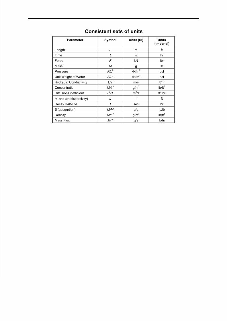
7/25/2019 Ctran Modeling
http://slidepdf.com/reader/full/ctran-modeling 101/101
Consistent sets of units
Parameter Symbol Units (SI) Units(Imperial)
Length L m ft
Time t s hrForce F kN lbf
Mass M g lb
Pressure F/L2 kN/m
2 psf
Unit Weight of Water F/L3 kN/m
3 pcf
Hydraulic Conductivity L/T m/s ft/hr
Concentration M/L3 g/m
3 lb/ft
3
Diffusion Coefficient L2 /T m
2/s ft
2/hr
αL and αT (dispersivity) L m ft
Decay Half-Life T sec hr
S (adsorption)M/M
g/g lb/lbDensity M/L
3 g/m
3 lb/ft
3
Mass Flux M/T g/s lb/hr


