31

1. Introduction

A central feature of the global economy is the extent of in-ternational imbalances, mainly the large and growing cur-rent account deficit of the United States. The sustainabilityof this situation as well as the pattern of an eventual adjust-ment are the subjects of substantial analysis and debate.Overall, however, a consensus has emerged that the inter-national imbalances are likely to unwind eventually, re-quiring a substantial adjustment in the exchange rate of thedollar. In a widely cited contribution, Obstfeld and Rogoff(2005, 2006) estimate that the dollar would have to depre-ciate by 30 to 38 percent against the world’s currencies toerase the U.S. current account deficit.

In this paper, we assess how the adjustment of the U.S.current account deficit interacts with the high degree offinancial integration in the world economy. In addition tomaking U.S. goods more competitive in world markets,hence helping U.S. exports, a depreciation of the dollarleads to a capital gain for the United States by boosting thedollar value of a given amount of its foreign-currency as-sets. This valuation channel is playing an increasingly largerole in driving the U.S. net investment position and, there-fore, in affecting the dynamics of international adjustment.

The magnitude of exchange rate movements, however,is only one dimension of the adjustment. Whether the adjustment is likely to take place gradually or suddenly re-mains an object of debate. Our analysis focuses on this dimension by considering an alternative experiment.Rather than immediately bringing the current account tozero, as Obstfeld and Rogoff do, we consider a scenariowhere U.S. net external debt is kept constant. We regardsuch a scenario as realistic, since the current level of U.S.net external debt has so far proved manageable. We findthat the presence of valuation effects allows for a “smoothlanding,” with the U.S. current account imbalance gradu-

Current Account Adjustment with High Financial Integration: A Scenario Analysis*

Michele Cavallo

EconomistFederal Reserve Bank of San Francisco

Cédric Tille

Senior EconomistFederal Reserve Bank of New York

A narrowing of the U.S. current account deficit through exchange rate movements is likely to entail a substantial deprecia-

tion of the dollar. We assess how the adjustment is affected by the high degree of international financial integration, with

exchange rate movements having a direct valuation impact on international assets and liabilities. In particular, a dollar de-

preciation generates a capital gain for the United States by boosting the value of its assets that are denominated in foreign

currencies. We consider an adjustment scenario in which the U.S. net external debt is held constant. One key finding is that

while the current account moves into balance, the pace of adjustment is smooth. Intuitively, the valuation gains stemming

from the depreciation of the dollar allow the United States to finance ongoing, albeit shrinking, current account deficits. We

find that the smooth pattern of adjustment is robust to alternative scenarios, although the ultimate movements in exchange

rates are affected.

*We thank Pierre-Olivier Gourinchas, Luca Guerrieri, Maurice Obst-feld, Alessandro Rebucci, Kenneth Rogoff, and Mark Spiegel for helpfulfeedback. Seminar participants at the Fall 2005 Federal Reserve SCIEAmeeting, the Graduate Institute of International Studies, Geneva (HEI),the University of Geneva, the University of Tübingen, the SwissNational Bank, and the Bank for International Settlements providedvaluable comments. We also thank Anita Todd for editorial assistance,and Thien Nguyen for excellent research assistance.

32 FRBSF Economic Review 2006

ally disappearing. Specifically, it takes three years for thecurrent account deficit to halve under our scenario.

Intuitively, the smooth pattern of the adjustment in ourscenario reflects the fact that the capital gains stemmingfrom the depreciation of the dollar are used to finance on-going, albeit shrinking, current account deficits during theadjustment. In the first year of the adjustment, the dollardepreciates, generating a capital gain through the valuationeffect. This gain is used to finance net imports, so the cur-rent account does not have to fall to zero immediately. Thisreduces the pressure on the exchange rate in the first year,with the dollar depreciating by only 9 percent. In the sec-ond year of the adjustment, this pattern is repeated, with afurther narrowing of the current account deficit, and a dol-lar depreciation reaching 15 percent from the initial situa-tion. Our adjustment scenario does ultimately bring thecurrent account into balance, as this is the only way to sta-bilize the U.S. net debt.

An important feature of our scenario is the leverage ininternational balance sheets. While net international assetpositions are constant, the values of gross assets and liabil-ities increase substantially. To assess the sensitivity of ourresults to this aspect, we complement our baseline scenarioby considering two alternatives. In the first one, we setfinancial flows to zero so leverage is kept constant. In thesecond one, we increase the rate of return on U.S. liabilitiesto match the rate on U.S. assets. The magnitude of ex-change rate movements is larger under both alternative sce-narios, and especially under the second alternative ofinterest rate convergence, where the dollar depreciation isboosted by one-third. Interestingly, the gradual nature ofadjustment remains robust, with the U.S. current accountdeficit only halving in three to four years. The compositionof adjustment is different from the baseline scenario, however. In particular the U.S. trade balance adjusts faster under the alternative scenarios, as the United Statesis no longer shielded from the interest burden on its liabilities.

The remainder of the paper is organized as follows.Section 2 provides background information and refers tothe literature on the topic. Section 3 presents the key ele-ments of our model. Section 4 describes our adjustmentscenario, as well as a sensitivity analysis to alternative sce-narios. Section 5 concludes.

2. Background and Literature Review

The large and growing current account deficit of the UnitedStates has become a central feature of the global economy,particularly in recent years. The U.S. external deficit in-creased gradually in the early 1990s, reaching a moderatelevel of 1.7 percent of GDP in 1997, and subsequently

widened at a fast pace, hitting 5.7 percent of GDP in 2004.This substantial borrowing from the rest of the world haspushed the United States into a substantial net debt vis-à-vis foreign investors, with net liabilities amounting to 21.7percent of GDP at the end of 2004.1

A volume by Clarida (2006) provides an overview of thesubstantial analysis and debate surrounding the sustainabil-ity of the U.S. external deficit and the path—whethersmooth or sudden—an eventual adjustment might take.Several economists argue that the current situation isdriven by policy choices that are likely to persist over sev-eral years, and that the United States is not condemned toface a disruptive adjustment in order to stabilize its borrow-ing.2 The United States may also have better growthprospects than the rest of the world, leading it to accountfor a permanently higher share of world GDP. In this situa-tion foreign investors could increase the share of U.S. as-sets in their portfolio, leading to sustained U.S. deficits,with a gradual adjustment once the portfolio reallocationhas run its course.3 Or, the U.S. financial sector may havean advantage in intermediating world savings. In this sce-nario, the transit of world savings through the UnitedStates to be converted into investment would lead to sus-tained current account imbalances.4

On the other side of the debate, many argue that the cur-rent situation is not sustainable and will lead to a substan-tial depreciation of the dollar vis-à-vis other currencies.This adjustment can be gradual and relatively benign.5

Several contributions, however, point to the risk of a rapidadjustment, with disruptive consequences for the worldeconomy.6 A representative, and widely cited contributionof the latter view is the work by Obstfeld and Rogoff(2005, 2006). They show that the return of the U.S. currentaccount deficit to balance entails a depreciation of the U.S.dollar of 30 to 35 percent against the main world curren-cies. In addition, they argue that such an adjustment couldtake place in a disruptive manner if it stemmed from for-eign investors losing confidence in the U.S. economy.

Exchange rate movements play a central role in mostscenarios of international adjustment. These movements

1. See Cavallo and Tille (2006) for data from the Bureau of EconomicAnalysis, International Economic Accounts.

2. See Dooley, Folkerts-Landau, and Garber (2005, 2006).

3. See Backus, Henriksen, Lambert, and Telmer (2005), and Engel andRogers (2006).

4. See Caballero, Farhi, and Gourinchas (2006).

5. See Blanchard, Giavazzi, and Sa (2005), Helbling, Batini, andCardarelli (2005), and Faruqee, Lexton, Muir, and Pesenti (2006).

6. See Roubini and Setser (2005).

Cavallo and Tille / Current Account Adjustment with High Financial Integration: A Scenario Analysis 33

affect the relative prices of various goods traded on theworld market; for example a weaker dollar would makeU.S. goods cheaper, hence boost U.S. exports. More im-portantly, exchange rate movements affect the price of nontraded goods (such as services) relative to traded goods(such as manufactured goods), inducing a reallocation ofconsumption between traded and nontraded goods.Obstfeld and Rogoff (2005, 2006) point out that this sec-ond channel plays a key role in the adjustment.

A growing body of research suggests that the degree offinancial integration has dramatically increased since theearly 1990s.7 The world has moved from a situation wherenet positions were dominant, with some countries beingcreditors and others being debtors, to a situation whereholdings of financial assets across countries have surged,with the values of gross assets and liabilities positionsdwarfing the values of net positions. This development hasopened a new channel through which exchange rate move-ments affect the world economies, the so-called valuationeffect. If countries are leveraged in terms of currencies,with the currency composition of their assets differingfrom that of their liabilities, exchange rate fluctuationshave a different effect on the two sides of the balance sheet,leading to sizable capital gains and losses in net terms.

This mechanism is illustrated by the case of the UnitedStates: while U.S. liabilities are nearly exclusively denom-inated in dollars, about two-thirds of U.S. assets are denominated in foreign currencies (Tille 2005). A depreci-ation of the dollar then improves the U.S. net investmentposition by increasing the dollar value of U.S. assets de-nominated in foreign currencies, while leaving the dollarvalue of U.S. liabilities essentially unchanged. This valua-tion channel has become an increasingly important factorin shaping the evolution of the U.S. net investment posi-tion. Indeed, over the last three years there developed anapparently puzzling pattern: the U.S. net international in-debtedness remained steady at 20 to 25 percent of GDP de-spite a current account deficit in the order of 5 percent ofGDP. This unusual pattern is a consequence of the valua-tion effect of exchange rate movements. While net finan-cial inflows required to fund the increasingly large currentaccount deficit consistently pushed the United States intodebt, the valuation effects of exchange rate movementsalso substantially affected the U.S. position. In particular,the depreciation of the dollar since 2002 generated capitalgains that amounted to about two-thirds of the current ac-count deficit, thereby significantly cushioning the deteri-

oration in the U.S. net investment position that arose fromthe need to finance the deficit.8

While some analyses of a narrowing of the U.S. currentaccount deficit take financial integration into account, theydo so in a way that limits its role.9 In particular, Obstfeldand Rogoff (2005, 2006) argue that taking the valuation ef-fect of exchange rate movements into account reduces therequired depreciation of the dollar only modestly. Thismodest effect reflects the exact nature of their experiment.Abstracting from valuation effects, the stabilization of U.S.net external debt at its current level requires the current ac-count to move into balance. When taking valuation effectsinto account, Obstfeld and Rogoff still require the currentaccount to move immediately into balance. This generatesa valuation effect that substantially improves the U.S. posi-tion, reducing the U.S. net external debt by a factor ofthree, but has a limited impact on the magnitude of the ex-change rate movement.

Another dimension of adjustment that is an importantfocus of our study is the pace of these movements. The ad-justment requires an eventual large depreciation of the dol-lar, and a contraction in U.S. consumption, as outlined byObstfeld and Rogoff (2005, 2006). If the adjustment weregradual, the reduction of consumption would not have tooccur immediately. In addition, a gradual adjustmentwould be less likely to be disruptive to financial markets.For instance, a 30 percent depreciation of the dollar wouldentail more adverse effects if concentrated over a year thanif smoothed over a decade.

3. A Three-Country Model of Interdependence

The main elements of our analysis are based on the workby Obstfeld and Rogoff (2005). In this section, we summa-rize these elements informally, and then focus on how oursetup departs from theirs. A more detailed presentation ofthe model is available in Cavallo and Tille (2006).

3.1. Consumption Allocation and Relative Prices

The model economy consists of three regions: the UnitedStates, Europe, and Asia, which are indexed by U, E, andA, respectively. The regions are linked by trade flows andby cross-holdings of financial instruments. Each regionproduces a traded good and a nontraded good, with thethree traded goods being imperfect substitutes. Aggregate

8. See Cavallo and Tille (2006) for details.

9. The valuation effects are incorporated into the analyses of Blanchardet al. (2005) and Obstfeld and Rogoff (2005, 2006).

7. See Gourinchas and Rey (2005, 2006), Lane and Milesi-Ferretti(2003, 2005, 2006), Obstfeld (2004), and Tille (2003, 2005).

34 FRBSF Economic Review 2006

consumption is first allocated between domestically pro-duced nontraded goods, Ci

N , and an index of the tradedgoods produced in all regions, Ci

T . The consumption indexof traded goods, Ci

T , includes the consumption of goodsproduced in the United States, Europe, and Asia, denotedby Ci

U , CiE , and Ci

A , respectively. The consumption in-dexes of traded goods in all regions include a home bias,with consumers’ preferences being tilted towards domesti-cally produced goods

The costs of the various consumption baskets are cap-tured by corresponding price indexes. These price indexesindicate the smallest amount of income required to pur-chase a unit quantity of the corresponding basket. Pi

C de-notes the consumer price index in country i, while Pi

N isthe price of nontraded goods and Pi

T is the price index oftraded goods in region i. For simplicity we use the U.S.currency as a numeraire in which prices are expressed. PU

T ,P E

T , and P AT are the price indexes of traded consumption in

the three regions expressed in dollars. Throughout this article we assume that all prices are fully flexible and thereare no impediments to trade, so that the price of a giventraded good is the same across the world.

Demand for the various goods in a given region is drivenby the aggregate consumption in the region, as well as thevarious relative prices. The bilateral terms-of-trade τi, j , isthe price of the traded good produced in region j, relative to the price of the traded good produced in region i. Thethree bilateral terms-of-trade in our setup are τU,A , τU,E ,and τE ,A . An increase in τU,E indicates a deterioration ofthe U.S. terms-of-trade vis-à-vis Europe, becauseEuropean-made goods are now more expensive in terms ofU.S.-produced goods. It can also be interpreted as a com-petitiveness gain for the United States vis-à-vis Europe.

A key relative price in region i is the price of the domes-tic nontraded goods relative to the price of the traded bas-ket in the region, xi . An increase in xi indicates that, inregion i, nontraded goods are more expensive in terms ofthe composite traded consumption basket.

The bilateral nominal exchange rates represent the valueof a currency in terms of another, with Ei, j being theamount of region i’s currency that is required to purchaseone unit of region j’s currency. We refer to the currencies ofthe United States, Europe, and Asia as the dollar, the euro,and the yen, respectively. The three bilateral nominal ex-change rates in our setup are EU,E , EU,A , and EE ,A , withan increase in EU,E reflecting a nominal depreciation ofthe dollar against the euro. The nominal exchange rates arecompleted by the real exchange rates, which represent theratios of consumer prices across countries. The three bilat-eral real exchange rates in our setup are qU,E , qU,A , andqE ,A . An increase in qU,E is an increase in the Europeanconsumer price index, relative to the United States. Such

an increase represents a real depreciation of the dollaragainst the euro, that is a depreciation of the U.S. currencythat is not offset by movements in the local currency priceindex. Bilateral real exchange rates are driven by both theterms-of-trade and the relative prices of nontraded goods.

An effective measure of the external value of a currencyis obtained by taking weighted averages of the various bi-lateral exchange rates. The three effective real exchangerates in our setup are qU, q E , and q A. An increase in qU

indicates that the dollar depreciates in real effective terms,reflecting a depreciation against the euro (an increase in qU,E ) or the yen (an increase in qU,A ).

While real exchange rates are driven entirely by relativeprices, namely the terms-of-trade and the relative prices ofnontraded goods, the nominal exchange rates are also af-fected by the level of prices in particular regions. Solvingfor nominal exchange rates then requires a specification ofmonetary policy to determine the price levels. We followObstfeld and Rogoff (2005) and assume that central bankskeep the price of a basket of domestically produced goodsconstant in local currency. We focus our discussion on realexchange rates, as the movements in nominal exchangerates are very similar.

3.2. International Financial Positions

A central feature of our analysis is the integration of finan-cial markets, with each region holding substantial asset positions in the other two regions.

3.2.1. Initial Asset and Liability Positions

Assets and liabilities on each region’s balance sheet con-sists of assets denominated in different currencies. Ex-change rate movements, then, affect asset values and leadto capital gains and losses across the three regions.Following Obstfeld and Rogoff (2005), we consider thatpositions are in a high-return bond paying an interest rate r W, except for the liabilities of the United States, whichare in a low-return dollar-denominated bond paying an in-terest rate rU < r W. This feature captures the “exorbitantprivilege” the United States enjoys in its ability to borrowfrom the rest of the world at lower rates than it faces whenlending (see Gourinchas and Rey 2006, and Lane andMilesi-Ferretti 2006).

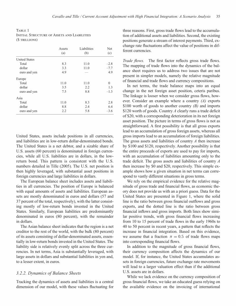
Table 1 summarizes the initial currency composition ofinternational balance sheets in the three regions derivedfrom those used by Obstfeld and Rogoff (2005).10 For the

10. For a more detailed illustration of the initial composition of assetsand liabilities, see Cavallo and Tille (2006).

Cavallo and Tille / Current Account Adjustment with High Financial Integration: A Scenario Analysis 35

United States, assets include positions in all currencies,and liabilities are in low-return dollar-denominated bonds.The United States is a net debtor, and a sizable share ofU.S. assets (60 percent) is denominated in foreign curren-cies, while all U.S. liabilities are in dollars, in the low-return bond. This pattern is consistent with the U.S. numbers detailed in Tille (2005). The U.S. net position isthen highly leveraged, with substantial asset positions inforeign currencies and large liabilities in dollars.

The European balance sheet includes assets and liabili-ties in all currencies. The position of Europe is balancedwith equal amounts of assets and liabilities. European as-sets are mostly denominated in euros and dollars (57 and37 percent of the total, respectively), with the latter consist-ing mostly of low-return bonds invested in the UnitedStates. Similarly, European liabilities are predominantlydenominated in euros (80 percent), with the remainder in dollars.

The Asian balance sheet indicates that the region is a netcreditor to the rest of the world, with the bulk (80 percent)of its assets consisting of dollar-denominated assets, essen-tially in low-return bonds invested in the United States. Theliability side is relatively evenly split across the three cur-rencies. In net terms, Asia is substantially leveraged, withlarge assets in dollars and substantial liabilities in yen and,to a lesser extent, in euros.

3.2.2. Dynamics of Balance Sheets

Tracking the dynamics of assets and liabilities is a centraldimension of our model, with these values fluctuating for

three reasons. First, gross trade flows lead to the accumula-tion of additional assets and liabilities. Second, the existingpositions generate a stream of interest payments. Third, ex-change rate fluctuations affect the value of positions in dif-ferent currencies.

Trade flows. The first factor reflects gross trade flows.The mapping of trade flows into the dynamics of the bal-ance sheet requires us to address two issues that are notpresent in simpler models, namely the relative magnitudeof financial and trade flows and currency compositions.

In net terms, the trade balance maps into an equalchange in the net foreign asset position, ceteris paribus.The linkage is looser when we consider gross flows, how-ever. Consider an example where a country (A) exports$100 worth of goods to another country (B) and imports$120 worth of goods. Country A clearly runs a trade deficitof $20, with a corresponding deterioration in its net foreignasset position. The picture in terms of gross flows is not asstraightforward. A first possibility is that all gross exportslead to an accumulation of gross foreign assets, whereas allgross imports lead to an accumulation of foreign liabilities.The gross assets and liabilities of country A then increaseby $100 and $120, respectively. Another possibility is thatthe entire proceeds of exports are used to pay for imports,with an accumulation of liabilities amounting only to thetrade deficit. The gross assets and liabilities of country Athen increase by $0 and $20, respectively. This simple ex-ample shows how a given situation in net terms can corre-spond to vastly different situations in gross terms.

We rely on the empirical evidence for the relative mag-nitude of gross trade and financial flows, as economic the-ory does not provide us with an a priori guess. Data for theUnited States are presented in Figure 1, where the solidline is the ratio between gross financial outflows and grossexports, and the dotted line is the ratio between grossfinancial inflows and gross imports. Both lines show simi-lar positive trends, with gross financial flows increasingfrom 10 to 15 percent of trade flows in the early 1960s to40 to 50 percent in recent years, a pattern that reflects theincrease in financial integration. Based on this evidence,we assume that a fraction π = 0.5 of trade flows mapsinto corresponding financial flows.

In addition to the magnitude of gross financial flows,their currency composition affects the dynamics of ourmodel. If, for instance, the United States accumulates as-sets in foreign currencies, future exchange rate movementswill lead to a larger valuation effect than if the additionalU.S. assets are in dollars.

While we lack evidence on the currency composition ofgross financial flows, we take an educated guess relying onthe available evidence on the invoicing of international

Table 1Initial Structure of Assets and Liabilities($ trillions)

Assets Liabilities Net(a) (b) (c)

United States Total 8.3 11.0 –2.8dollar 3.3 11.0 –7.7euro and yen 4.9 — 4.9

EuropeTotal 11.0 11.0 0dollar 3.5 2.2 1.3euro and yen 7.5 8.8 –1.3

AsiaTotal 11.0 8.3 2.8dollar 8.8 2.4 6.4euro and yen 2.2 5.8 –3.6

36 FRBSF Economic Review 2006

trade flows, as reported by Goldberg and Tille (2005).11 Weassume that trade flows to and from the United States leadpredominantly to an accumulation of dollar assets and lia-bilities.12 Trade flows between Europe and Asia lead prima-rily to an accumulation of positions in euros, with a sizablesecondary role for dollar positions.

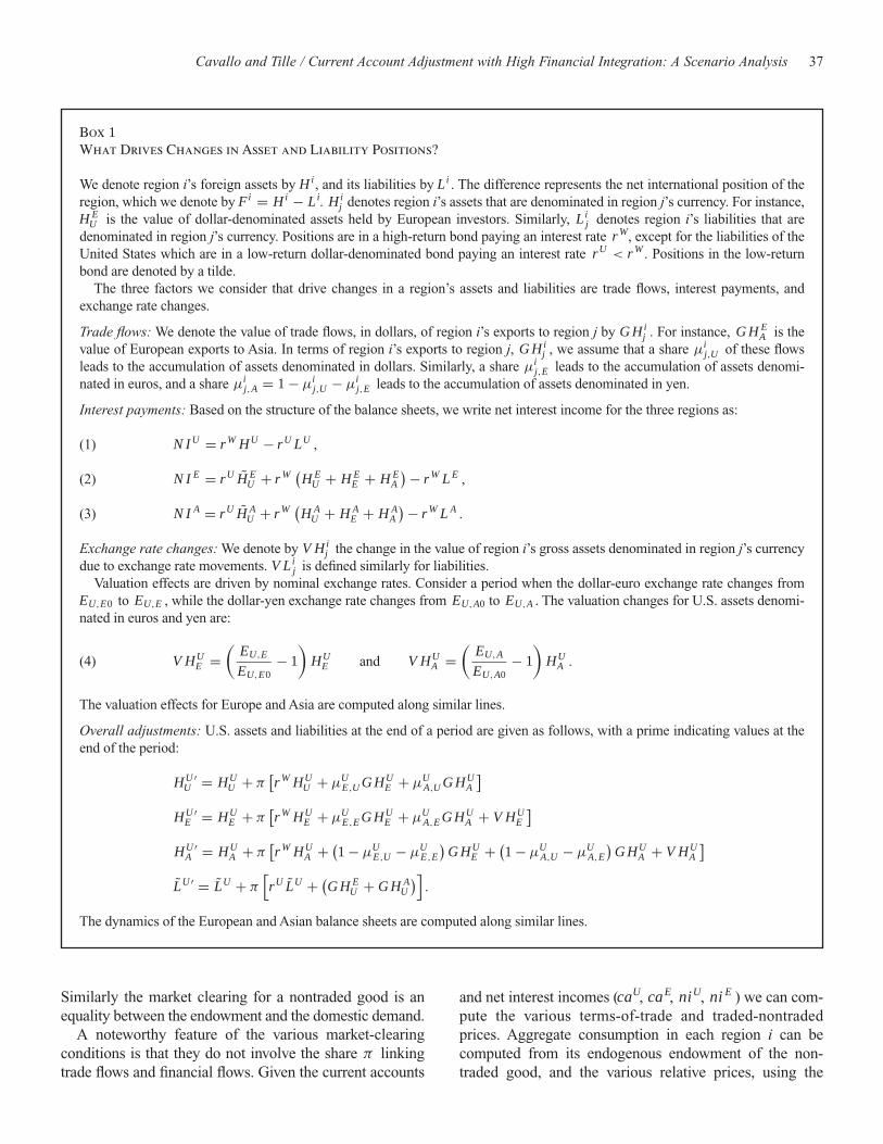
Interest payments and valuation gains. The second driv-er of changes in assets and liabilities is the flow of interestincome. For simplicity, we assume that a share π of theproceeds from interest payments are simply added to theprincipal of the corresponding position, with π being thesame as the share of gross trade flows that map into finan-cial flows. The net interest income for each region is thedifference between the interest earned on its assets and thatpaid on its liabilities. See Box 1 for details.

The final driver of balance sheet dynamics is the valua-tion effect stemming from exchange rate movements. Aswe express all positions in dollars, there is no such effectfor the positions in dollar-denominated assets. However,the dollar value of positions in euro- or yen-denominatedassets is affected. We again assume that a share π of thesevaluation effects is added to the principal of the correspon-ding positions.

Overall dynamics and consistency. The dynamics of thevarious exchange rates are given by combining the threechannels, as shown in Box 1.

While the assumption that trade flows, interest income,and valuation gains all map into gross positions up to ascaling π simplifies our model, one may worry that itcould lead to inconsistencies across the various assets andliabilities. In Box 2 we show that this is not the case in theparticular scenario we consider. As our scenario analysisfocuses on constant net asset positions, our scaling of grossflows and valuations by π across the board is fine, thoughit would be problematic for other scenarios.

Aggregating the various components of balance sheetdynamics, the changes in the net foreign asset positions ofthe various countries are the sums of the current accountsand the valuation effects on assets and liabilities, as shownin Box 2.

3.3. Market-Clearing Conditions

In each region, the current account, in dollars, is the sum ofnet interest income and the trade balance, the latter beingthe difference between the value of tradable output and thevalue of consumption of tradable goods. For simplicity, thesupply side of the world economy is modeled as an endow-ment economy.

We denote the endowments of tradable and nontradedgoods in region i by Y i

T and Y iN , respectively. Note that the

valuation effects of exchange rate movements, VH and VL,do not enter the current account as they do not entail anyfinancial flows across countries. Region i’s current accountis then C Ai = N I i + Pi Y

iT − Pi

T CiT .

The clearing of goods markets requires that the endow-ments of the various goods are equal to the sum of domes-tic and foreign consumptions which depend on aggregateconsumptions in the various regions and on relative prices.We define the following ratios between the various endow-ments of tradable and nontraded goods: σU/E = Y U

T /Y ET ,

σU/A = Y UT /Y A

T , and σN/ i = Y iN /Y i

T . We use lower-case variables to denote the ratio between a dollar valueand the value of the endowment of U.S. tradable good,PU Y U

T . We scale the various trade flows in this way:ghi

j = G Hij /(PU Y U

T ) . Net interest incomes and currentaccounts are similarly scaled, with ni i = N I i/PU Y U

T andcai = C Ai/PU Y U

T .Using the allocation of consumption across the various

goods, we write the various trade flows in terms of relativeprices (the terms-of-trade and price between traded andnontraded goods) and the trade balance (current accountnet of interest income). The market-clearing condition for aparticular traded good states that the endowment of thegood is equal to the sum of domestic and foreign demands.

11. While a flow can be invoiced in one currency and transacted in an-other, we posit that the invoicing currency is a good indicator of thetransaction currency.

12. Details are given in Cavallo and Tille (2006). The accumulation ofU.S. liabilities takes place in the low-return dollar bond.

Figure 1Ratio of Gross Financial Flows to Gross Trade Flows

0

10

20

30

40

50

60

70

60 64 68 72 76 80 84 88 92 96 00 04

Outflows/Exports

Inflows/Imports

Percent

Source: Bureau of Economic Analysis, International Economic Accounts.

Cavallo and Tille / Current Account Adjustment with High Financial Integration: A Scenario Analysis 37

Similarly the market clearing for a nontraded good is anequality between the endowment and the domestic demand.

A noteworthy feature of the various market-clearingconditions is that they do not involve the share π linkingtrade flows and financial flows. Given the current accounts

and net interest incomes (caU, caE, niU, ni E ) we can com-pute the various terms-of-trade and traded-nontradedprices. Aggregate consumption in each region i can becomputed from its endogenous endowment of the non-traded good, and the various relative prices, using the

Box 1What Drives Changes in Asset and Liability Positions?

We denote region i’s foreign assets by Hi, and its liabilities by Li . The difference represents the net international position of theregion, which we denote by Fi = Hi − Li. Hi

j denotes region i’s assets that are denominated in region j’s currency. For instance,H E

U is the value of dollar-denominated assets held by European investors. Similarly, Lij denotes region i’s liabilities that are

denominated in region j’s currency. Positions are in a high-return bond paying an interest rate r W, except for the liabilities of theUnited States which are in a low-return dollar-denominated bond paying an interest rate rU < r W . Positions in the low-returnbond are denoted by a tilde.

The three factors we consider that drive changes in a region’s assets and liabilities are trade flows, interest payments, and exchange rate changes.

Trade flows: We denote the value of trade flows, in dollars, of region i’s exports to region j by G Hij . For instance, G H E

A is thevalue of European exports to Asia. In terms of region i’s exports to region j, G Hi

j , we assume that a share µij,U of these flows

leads to the accumulation of assets denominated in dollars. Similarly, a share µij,E leads to the accumulation of assets denomi-

nated in euros, and a share µij,A = 1 − µi

j,U − µij,E leads to the accumulation of assets denominated in yen.

Interest payments: Based on the structure of the balance sheets, we write net interest income for the three regions as:

(1) N I U = r W HU − rU LU ,

(2) N I E = rU H̃ EU + r W

(H E

U + H EE + H E

A

) − r W L E ,

(3) N I A = rU H̃ AU + r W

(H A

U + H AE + H A

A

) − r W L A .

Exchange rate changes: We denote by V Hij the change in the value of region i’s gross assets denominated in region j’s currency

due to exchange rate movements. V Lij is defined similarly for liabilities.

Valuation effects are driven by nominal exchange rates. Consider a period when the dollar-euro exchange rate changes fromEU,E0 to EU,E , while the dollar-yen exchange rate changes from EU,A0 to EU,A . The valuation changes for U.S. assets denomi-nated in euros and yen are:

(4) V HUE =

(EU,E

EU,E0− 1

)HU

E and V HUA =

(EU,A

EU,A0− 1

)HU

A .

The valuation effects for Europe and Asia are computed along similar lines.

Overall adjustments: U.S. assets and liabilities at the end of a period are given as follows, with a prime indicating values at theend of the period:

HU ′U = HU

U + π[r W HU

U + µUE,U G HU

E + µUA,U G HU

A

]

HU ′E = HU

E + π[r W HU

E + µUE,E G HU

E + µUA,E G HU

A + V HUE

]

HU ′A = HU

A + π[r W HU

A + (1 − µU

E,U − µUE,E

)G HU

E + (1 − µU

A,U − µUA,E

)G HU

A + V HUA

]

L̃U ′ = L̃U + π[rU L̃U + (

G H EU + G H A

U

)].

The dynamics of the European and Asian balance sheets are computed along similar lines.

38 FRBSF Economic Review 2006

demand for nontraded goods. The share π matters only inmapping the ensuing results into the dynamics of the vari-ous components of the international balance sheets.

3.4. Solution Method

Our solution method computes the various prices in a pe-riod based on the initial international balance sheets andstructural parameters. The results are then mapped into thedynamics of the balance sheet to compute a new set of in-ternational assets and liabilities that underpin the solutionfor the following period.

Given an initial structure of assets and liabilities and ini-tial nominal exchange rates, we can easily compute the netinterest incomes in Box 1, equations (1) to (3). We thenpick values for the U.S. and European current accounts indollars, C AU and C AE, and the endowment of U.S. trad-able goods, Y U

T . The values of the various current accountbalances are not freely picked. As we aim for constant netasset positions, we iterate our procedure so the current ac-counts lead to constant positions. Similarly, the endow-ment of U.S. tradable goods is computed based on thecurrent allocation (as in Obstfeld and Rogoff 2005) andthen held constant.

Box 2Net Financial Flows

Focusing on the United States for brevity, net financial flows consist of two main components. The first is the proceeds of tradeflows and net interest payments that are added to net assets (which are a share π of these flows). The second is the share (1 − π )of valuation gains that is not added to the principal of the corresponding positions, bearing in mind that a valuation gain that isbrought back into the United States is a financial inflow, that is, a negative financial flow. Net financial flows are then:

F FU = π[(

G HUE + G HU

A

) − (G H E

U + G H AU

) + N I U] − (1 − π)

(V HU

E + V HUA

)= πC AU − (1 − π)

(V HU

E + V HUA

),

where C AU is the U.S. current account, that is the overall net trade and interest payments flow. Net financial flows and current accounts are equal, as they should be, only when:

F FU = C AU = πC AU − (1 − π)(V HU

E + V HUA

) ⇒ C AU = − (V HU

E + V HUA

).

Therefore, our assumption that π is the same across the board is valid only when the current account is the inverse of the capitalgains, that is when capital gains are associated with a current account deficit. A complementary way to establish this point is tolook at the dynamics of the net foreign asset position. In our setup, the change in the net foreign asset position is the sum of theproceeds from trade flows and from net interest payments that are added to net assets, and the valuation gains that are added to the corresponding positions:

(5) FU ′ − FU = πC AU + π(V HU

E + V HUA

).

The changes in the net positions in the data, such as those published by the Bureau of Economic Analysis, combine the current account and the valuation effects:

(6)(FU ′ − FU

)BEA = C AU + (

V HUE + V HU

A

).

Comparing (5) and (6) clearly shows that the dynamics of net foreign assets are inconsistent in general. The notable exception isthe case where net foreign assets are constant:

(FU ′ − FU

)BEA = (

FU ′ − FU) = 0 . In this case, the trade flows, interest income,

and valuation effects sum to zero, whether or not they are all multiplied by π .The changes in the net foreign asset positions for each region are

(7) 0 = C AU + (V HU

E + V HUA

),

(8) 0 = C AE + (V H E

E + V H EA

) − (V L E

E + V L EA

),

(9) 0 = C AA + (V H A

E + V H AA

) − (V L A

E + V L AA

).

Cavallo and Tille / Current Account Adjustment with High Financial Integration: A Scenario Analysis 39

Armed with the values for the U.S. and European cur-rent accounts, the net interest income, and the endowmentof U.S. tradable goods, we compute the terms-of-tradeτU,A and τU,E , the relative prices of nontraded goods, xU, x E, and x A, and the price of the U.S. tradable good, PU.This is done by numerically solving a system including themarket-clearing conditions, and the expression for theprice of the U.S. tradable good. Having solved the variousrelative prices, the real and nominal exchange rates easilyfollow. Combining the nominal exchange rates with theones taken from the previous period, we compute the valu-ation effects on assets and liabilities. Combining the tradeflows, interest income, and valuation effects, we computethe dynamics of the balance sheets, using the scaling factorπ . These new asset and liability positions serve as the basisfor the solution in the following period.

Note that the dynamic dimension of our analysis comessolely through the dynamics of the international balancesheets. For instance, consumption is not computed from anintertemporal optimization but is given by the exogenousendowments and the current account, the latter being set byour assumption of the dynamics of net foreign assets.

4. Global Adjustment under Various Scenarios

Our parameter values are as in Cavallo and Tille (2006),and we follow Obstfeld and Rogoff (2005) as much as pos-sible. We assume that half the gross trade flows map intofinancial flows (π = 0.5) as is the case in the United Statescurrently (Figure 1). We consider two extensions: one withno accumulation of assets and liabilities beyond the currentpositions (π = 0), and one where the interest rate on U.S.liabilities, rU, increases from 3.75 percent to 5 percent tomatch the world interest rate, r W.

4.1. Static Scenarios

We start by briefly reviewing the results of Obstfeld andRogoff (2005). They consider static scenarios in the sensethat the current accounts in all countries return to zero im-mediately.13 The first column of Table 2 shows the main re-sults for their analysis. The top section indicates the realdepreciation of the dollar against the other currencies,while the bottom section shows the effective real deprecia-

tions of the various currencies (the movements in nominalexchange rates are very similar).14

Column (a) in Table 2 shows a scenario that entirely ab-stracts from any valuation effect, that is, a scenario whereall assets and liabilities are denominated in dollars. Theglobal rebalancing of the world economy requires a sharpdepreciation of the dollar of 38 percent in effective terms,mirrored mainly by a substantial yen appreciation.Obstfeld and Rogoff (2005) also consider valuation effects,a case presented in column (b) of Table 2. Their exact sce-nario still requires all current accounts to move to zero. Theadjustment entails a substantial depreciation of the dollar.This, in turn, generates a substantial capital gain for theUnited States, with its net debt falling by 70 percent,mostly at the expense of Asia. This improves the net inter-est income of the United States, and the trade balance doesnot have to narrow as much in order to bring the current ac-count into balance. This, in turn, reduces the required move-ment in the exchange rate. Obstfeld and Rogoff (2005)argue that the benefits from the valuation effect are second-ary, as the dollar still has to depreciate by 33 percent.

4.2. A Dynamic Scenario

The limited impact of the valuation effect on the exchangerate in Obstfeld and Rogoff (2005) is a consequence ofusing the valuation gain to reduce the U.S. net debt whilestill requiring an immediate adjustment in the current ac-count. This is only one of several possible uses of the valu-ation gains, and our analysis focuses on an alternativescenario where net international investment positions areheld constant in all three regions. We regard this scenarioas a reasonable alternative, as the U.S. net external debt hasremained essentially unchanged in the last three years at alevel that has so far proved manageable. In our scenario,the valuation effects stemming from exchange rate move-ments allow the various regions to run current account sur-pluses and deficits. These imbalances are financed byvaluation gains and losses, keeping international invest-ment positions constant, as shown by equations (7) to (9) inBox 2.

Our scenario highlights two dimensions of adjustment,namely the pace of adjustment and the ultimate movementsin the various variables. Equation (4) in Box 1 shows thatvaluation effects require movements in nominal exchangerates. In the long run, once adjustment has run its course,the economy reaches a new steady state where all vari-

13. Obstfeld and Rogoff (2005) do not present their scenario as the ad-justment taking place in one period, but rather in terms of comparing thecurrent situation with a steady state where net positions are constant.However, as they abstract from any dynamics, their scenarios implicitlyassume an immediate adjustment.

14. The numbers in Table 2 differ slightly from the ones presented inObstfeld and Rogoff (2005), because we consider a structure of assetsand liabilities in Table 2 that is slightly different from the one they use.

40 FRBSF Economic Review 2006

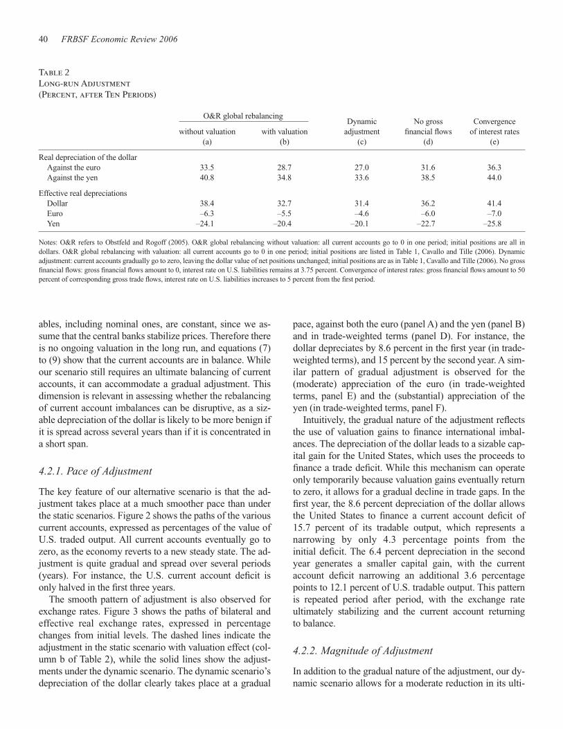
ables, including nominal ones, are constant, since we as-sume that the central banks stabilize prices. Therefore thereis no ongoing valuation in the long run, and equations (7)to (9) show that the current accounts are in balance. Whileour scenario still requires an ultimate balancing of currentaccounts, it can accommodate a gradual adjustment. Thisdimension is relevant in assessing whether the rebalancingof current account imbalances can be disruptive, as a siz-able depreciation of the dollar is likely to be more benign ifit is spread across several years than if it is concentrated ina short span.

4.2.1. Pace of Adjustment

The key feature of our alternative scenario is that the ad-justment takes place at a much smoother pace than underthe static scenarios. Figure 2 shows the paths of the variouscurrent accounts, expressed as percentages of the value ofU.S. traded output. All current accounts eventually go tozero, as the economy reverts to a new steady state. The ad-justment is quite gradual and spread over several periods(years). For instance, the U.S. current account deficit isonly halved in the first three years.

The smooth pattern of adjustment is also observed forexchange rates. Figure 3 shows the paths of bilateral andeffective real exchange rates, expressed in percentagechanges from initial levels. The dashed lines indicate theadjustment in the static scenario with valuation effect (col-umn b of Table 2), while the solid lines show the adjust-ments under the dynamic scenario. The dynamic scenario’sdepreciation of the dollar clearly takes place at a gradual

pace, against both the euro (panel A) and the yen (panel B)and in trade-weighted terms (panel D). For instance, thedollar depreciates by 8.6 percent in the first year (in trade-weighted terms), and 15 percent by the second year. A sim-ilar pattern of gradual adjustment is observed for the(moderate) appreciation of the euro (in trade-weightedterms, panel E) and the (substantial) appreciation of theyen (in trade-weighted terms, panel F).

Intuitively, the gradual nature of the adjustment reflectsthe use of valuation gains to finance international imbal-ances. The depreciation of the dollar leads to a sizable cap-ital gain for the United States, which uses the proceeds tofinance a trade deficit. While this mechanism can operateonly temporarily because valuation gains eventually returnto zero, it allows for a gradual decline in trade gaps. In thefirst year, the 8.6 percent depreciation of the dollar allowsthe United States to finance a current account deficit of15.7 percent of its tradable output, which represents a narrowing by only 4.3 percentage points from the initial deficit. The 6.4 percent depreciation in the secondyear generates a smaller capital gain, with the current account deficit narrowing an additional 3.6 percentagepoints to 12.1 percent of U.S. tradable output. This patternis repeated period after period, with the exchange rate ultimately stabilizing and the current account returning to balance.

4.2.2. Magnitude of Adjustment

In addition to the gradual nature of the adjustment, our dy-namic scenario allows for a moderate reduction in its ulti-

Table 2Long-run Adjustment(Percent, after Ten Periods)

O&R global rebalancing Dynamic No gross Convergence

without valuation with valuation adjustment financial flows of interest rates(a) (b) (c) (d) (e)

Real depreciation of the dollarAgainst the euro 33.5 28.7 27.0 31.6 36.3Against the yen 40.8 34.8 33.6 38.5 44.0

Effective real depreciationsDollar 38.4 32.7 31.4 36.2 41.4Euro –6.3 –5.5 –4.6 –6.0 –7.0Yen –24.1 –20.4 –20.1 –22.7 –25.8

Notes: O&R refers to Obstfeld and Rogoff (2005). O&R global rebalancing without valuation: all current accounts go to 0 in one period; initial positions are all in dollars. O&R global rebalancing with valuation: all current accounts go to 0 in one period; initial positions are listed in Table 1, Cavallo and Tille (2006). Dynamic adjustment: current accounts gradually go to zero, leaving the dollar value of net positions unchanged; initial positions are as in Table 1, Cavallo and Tille (2006). No grossfinancial flows: gross financial flows amount to 0, interest rate on U.S. liabilities remains at 3.75 percent. Convergence of interest rates: gross financial flows amount to 50percent of corresponding gross trade flows, interest rate on U.S. liabilities increases to 5 percent from the first period.

Cavallo and Tille / Current Account Adjustment with High Financial Integration: A Scenario Analysis 41

mate magnitude. Column (c) of Table 2 shows the magni-tude of depreciation in our dynamic scenario after ten peri-ods. While the dollar still substantially depreciates, themagnitude is reduced to 31 percent. The depreciation of thedollar is therefore reduced by nearly one-fifth compared tothe static scenario that ignores valuation effects (where thedollar depreciates by 38 percent). This magnitude isbroadly consistent with the results in Gourinchas and Rey(2005), who find that valuation effects stemming from ex-change rate movements account for one-third of the histor-ical adjustment of U.S. external imbalances. Using a richermulti-country model, Helbling, Batini, and Cardarelli(2005) argue that higher financial integration facilitates theprocess of current account adjustment. Compared to thestatic case including valuation effects, our dynamic sce-nario shows a moderate dampening, with the depreciationof the dollar being reduced by 4 percent in effective terms.

4.2.3. The Impact on International Balance Sheets

Our adjustment scenario implies substantial valuation ef-fects for international assets and liabilities. The substantialdepreciation of the dollar results in a large capital gain forthe United States, amounting to $1.8 trillion for the first tenyears after the adjustment started. This comes essentially atthe expense of Asia, which suffers a loss of $1.4 trillion,while Europe faces a moderate capital loss. The high expo-

sure of Asia to capital loss is consistent with the findings ofHiggins and Klitgaard (2004).

The combination of trade flows, interest income, andvaluation effects leads to substantial movements in interna-tional balance sheets. While the net positions are un-changed by assumptions, the gross asset and liabilitypositions essentially double over ten years.15 This repre-sents a sizable increase in leverage but is consistent withempirical evidence. Between 1994 and 2004, U.S. grossassets nearly doubled from 47 percent to 85 percent ofGDP, while liabilities increased even more from 49 percentto 107 percent.

4.3. Sensitivity Analysis: Alternative Scenarios

We complete our baseline scenario by considering two ex-tensions. In the first we assume that all gross financialflows are netted out (π = 0), so that gross assets and liabil-ities are held constant at their initial levels. This alternativewith no gross financial flows illustrates the influence of theincrease of gross positions on our results. In the second ex-tension we assume that the U.S. exorbitant privilege disap-pears, with the interest rate on the low-return dollar bonds,rU, immediately increasing to the world interest rate, r W

(this scenario holds π at 0.5). This second alternative withconvergence of interest rates allows us to weight the gainsfrom valuation effects against the interest burden of theU.S. net debt.

4.3.1. Pace and Magnitude of Adjustment

The gradual nature of the adjustment is observed across allscenarios, and, therefore, is robust to the alternatives.Adjustment is slower under interest rate convergence, butthe gap is small and entirely reflects the jump in interestrate in the first period. The pace of exchange rate adjust-ment also remains gradual, although the ultimate magni-tude of adjustment (after ten years) is sensitive to ouralternatives. Column (d) of Table 2 shows the exchangerate movements under the alternative with no gross finan-cial flows. The magnitude of adjustment is substantially in-creased, with the dollar depreciating by 36 percent ineffective terms, an increase by one-sixth compared to thebaseline scenario.

The magnitude of the ultimate adjustment is also sensi-tive to the path of interest rates, with exchange rate move-ments being larger under the alternative of convergence(column e). The dollar now depreciates by 41 percent in ef-fective terms, a one-third increase compared to the baselinescenario. The sensitivity to interest rates goes beyond the

Figure 2Current Accounts, Baseline Scenario

-20

-15

-10

-5

0

5

10

15

20

0 1 2 3 4 5 6 7 8 9 10

Asia

Europe

United States

Percent of U.S. traded output

Periods (years)

15. See Cavallo and Tille (2006) for details.

42 FRBSF Economic Review 2006

Figure 3Real Exchange Rate Movements

0

5

10

15

20

25

30

35

0 2 4 6 8 10

A. Depreciation of the dollar against the euro

Percent changes

O&R global rebalancing

Dynamicadjustment

Period

0

5

10

15

20

25

30

35

0 2 4 6 8 10

D. Depreciation of the trade-weighted dollar

Percent changesO&R global rebalancing

Dynamicadjustment

Period

0

5

10

15

20

25

30

35

0 2 4 6 8 10

C. Depreciation of the euro against the yen

Percent changes

Dynamicadjustment

O&R global rebalancing

Period

-25

-20

-15

-10

-5

0

0 2 4 6 8 10

E. Depreciation of the trade-weighted euro

Percent changes

Dynamicadjustment

O&R global rebalancing

Period

-25

-20

-15

-10

-5

0

0 2 4 6 8 10

F. Depreciation of the trade-weighted yen

Percent changes

Dynamicadjustment

O&R global rebalancing

Period

0

5

10

15

20

25

30

35

40

0 2 4 6 8 10

B. Depreciation of the dollar against the yen

Percent changes

Dynamicadjustment

O&R global rebalancing

Period

Note: Percent change refers to percent change from current situation. Periods are in years. O&R refers to Obstfeld and Rogoff (2005).

Cavallo and Tille / Current Account Adjustment with High Financial Integration: A Scenario Analysis 43

impact computed by Obstfeld and Rogoff (2005), who findthat a convergence moderately increases the depreciationof the dollar vis-à-vis the euro (from 28.6 to 30.1 percent).This difference in our results reflects two aspects. First,Obstfeld and Rogoff (2005) assume that the convergenceapplies only to U.S. debt in short-duration bonds, whichrepresents only 30 percent of U.S. liabilities. Second, ourassumption that gross positions increase (π > 0) impliesan increasing and costly leverage for the United States.This dimension is substantial, as the gross positions doubleunder the alternative scenario.

4.3.2. The Composition of Adjustment

While the adjustment of the current account shows littledifference across our baseline scenario and the two alterna-tives we consider, the components of the current accountare more contrasted. Table 3 summarizes the overall adjust-ment over the ten periods we consider. The top section in-dicates the cumulative valuation gains for the three regions.Under the baseline adjustment (column a), the depreciationof the dollar leads to a $1.8 trillion capital gain for theUnited States, allowing it to finance a gradual rebalancingof the current account. The U.S. gain is mirrored primarilyby a loss in Asia. The valuation effect is essentially un-changed in the absence of gross flows (column b). In the al-ternative with a convergence of interest rates, the valuationeffects are magnified, amounting to $2.5 trillion, i.e., $0.7trillion more than in the baseline scenario.

The valuation gains and losses exactly correspond to thecumulative current account under our assumption that netasset positions are constant. The cumulative current ac-counts are in turn the sum of net interest income and thetrade balance, which are presented in the middle and bot-tom sections of Table 3. Under the baseline scenario, theUnited States benefits from net interest income, despitebeing a net debtor, because it earns a larger return on its as-sets than it pays on its liabilities. This interest transfercomes essentially at the expense of Europe, while the netassets of Asia are large enough to offset its earning a lowerrate on its assets than it pays on its liabilities. As a result ofthis “exorbitant privilege,” the United States can run a cu-mulative trade deficit ($2.2 trillion) that exceeds its cumu-lative current account deficit ($1.8 trillion). This limits thepressure on the exchange rate, which is driven primarily bythe required adjustment in the trade balance.

The cumulative current accounts are essentially thesame in the alternative with no financial flows: they aredriven more by trade balances. The United States earns nonet interest income, so the rebalancing requires a smallertrade deficit ($1.8 trillion) than under the baseline scenario($2.2 trillion). In the absence of gross flows, the United

States cannot increase its leverage between high-return as-sets and low-return liabilities, which limits its interest in-come. As more of the adjustment comes through the tradebalance, the dollar depreciates more under this alternative.

While the United States runs a larger cumulative currentaccount deficit in the alternative with interest rate conver-gence ($2.5 trillion) than in the baseline ($1.8 trillion), thisis merely a reflection of the large movement of the ex-change rate due to the interest burden of U.S. liabilities.The increase in the interest rate that the United States payson these liabilities removes its “exorbitant privilege,” andthe net debt translates into substantial net interest pay-ments. Compared to the baseline scenario, the UnitedStates pays $1.4 trillion in net interest. This represents a$1.8 trillion shift from the baseline scenario, where theUnited States was receiving a net interest income of $0.4trillion. While the country benefits from a larger valuationgain ($2.5 trillion, compared to $1.8 trillion in the base-line), the extra gain is too small to offset the surge in the in-terest burden. The burden then requires a faster narrowingof the trade deficit, with the cumulative trade deficitamounting to $1.2 trillion, i.e., half of its value under thebaseline case. The faster narrowing in the trade deficit re-quires a larger depreciation of the dollar. Note that the pres-ence of valuation effects still smooths the adjustment. Withthe valuation effect, the difference in the trade balancefrom the baseline scenario ($1.0 trillion) amounts to 60

Table 3Cumulative Flows and Valuation Gains($ trillions)

Baseline dynamic No gross Convergence ofadjustment financial flows interest rates

(a) (b) (c)

Cumulative valuation gainU.S. 1.82 1.80 2.52Europe –0.38 –0.36 –0.56Asia –1.44 –1.44 –1.96

Cumulative net interest incomeU.S. 0.41 0.00 –1.38Europe –0.52 –0.38 0Asia 0.11 0.38 1.38

Cumulative trade balanceU.S. –2.23 –1.80 –1.15Europe 0.89 0.74 0.56Asia 1.33 1.06 0.59

Notes: All amounts represent total amounts between the initial period and periodten. Valuation gain: total amounts transferred through the valuation effect of ex-change rate movements. Net interest income: total amounts transferred throughinterest receipts net of payments. Trade balance: total amounts transferredthrough exports net of imports.

44 FRBSF Economic Review 2006

percent of the additional interest payments ($1.8 trillion),while in the absence of these effects the trade balancewould have to match the additional interest payments ex-actly. The sensitivity of U.S. external accounts to alterna-tive scenarios for the returns on assets and liabilities is inline with the results of Higgins, Klitgaard, and Tille (2005).

5. Concluding Remarks

The rapidly widening U.S. current account deficit has re-ceived a lot of attention, with several economists pointingout that bringing the current account down to a more sus-tainable level could require a substantial, and possibly dis-ruptive, depreciation of the dollar. This paper assesses howsuch an adjustment would be affected by the high degree offinancial integration across countries. The main conse-quence of financial integration is the growing relevance ofvaluation effects, where exchange rate movements lead tosizable changes in the value of a country’s assets and liabil-ities. We consider an adjustment scenario where current ac-count imbalances are resorbed, and the net asset positionsof the various countries are kept constant.

Our main finding is that high financial integration canpotentially generate a “smooth landing” pattern, with avery gradual movement of the current accounts into bal-ance. Focusing on the United States in our model, the de-preciation of the dollar generates capital gains, which canbe used to finance a narrowing current account deficitwhile keeping the net debt vis-à-vis the rest of the worldunchanged. The pace of adjustment is an important featureof the rebalancing scenario. One of the main concerns inunwinding the current account imbalance is that the adjust-

ment may prove sudden and disorderly, with foreign in-vestors losing confidence in the United States, for instance.Obstfeld and Rogoff (2005) focus on the risk of a “hardlanding,” where the depreciation of the dollar that they cal-culate would take place in a fast and disruptive manner.While a 30 percent depreciation of the dollar in a singleyear could be disruptive for world markets, a similar move-ment spread over several years would be more manage-able. Our scenario explores a situation in which the largestone-year depreciation of the dollar is less than 10 percent, amagnitude that can be absorbed by markets: in 2003 and2004 the dollar depreciated by 12.2 and 8.2 percent (asmeasured by the major currency index published by theFederal Reserve Board of Governors),16 a movement thatproved manageable.

A sensitivity analysis shows that the gradual pace of adjustment, which is the central result of our analysis, re-mains robust to alternative scenarios. However, the magni-tude of the exchange rate movements is larger if we limitgross financial flows, thereby limiting the leverage be-tween assets and liabilities with different rates of return.The United States also benefits from earning a larger returnon its assets than it pays on its liabilities, and removing thisspread leads to a larger adjustment in the exchange rate.

A caveat to our setup is that the dynamic linkages re-main quite simple, as we do not consider any intertemporaloptimization by agents. Nevertheless, several studies, suchas Blanchard et al. (2005), Helbling et al. (2005), andFaruqee et al. (2006), use richer models of the world econ-omy and find a gradual adjustment to be a manageable alternative.

16. The values of the index are 105.98 (2002), 93.04 (2003), and 85.42(2004). See http://www.federalreserve.gov/releases/g5a/current/.

Cavallo and Tille / Current Account Adjustment with High Financial Integration: A Scenario Analysis 45

References

Backus, David, Espen Henriksen, Frederic Lambert, and Chris Telmer.2005. “Current Account Fact and Fiction.” Manuscript. New YorkUniversity.

Blanchard, Olivier, Francesco Giavazzi, and Filipa Sa. 2005. “Inter-national Investors, the U.S. Current Account and the Dollar.”Brookings Papers on Economic Activity 2005(1) pp. 1–49.

Caballero, Ricardo, Emmanuel Farhi, and Pierre-Olivier Gourinchas.2006. “An Equilibrium Model of ‘Global Imbalances’ and LowInterest Rates.” NBER Working Paper 11996 (February).

Cavallo, Michele, and Cédric Tille. 2006. “Could Capital Gains Smootha Current Account Rebalancing?” FRB San Francisco WorkingPaper 2006-03 (February). http://www.frbsf.org/publications/economics/papers/2006/wp06-03bk.pdf

Clarida, Richard H., editor. 2006. G-7 Current Account Imbalances:Sustainability and Adjustment. Chicago: University of ChicagoPress, forthcoming.

Dooley, Michael P., David Folkerts-Landau, and Peter M. Garber. 2005.“Saving Gluts and Interest Rates: The Missing Link to Europe.”NBER Working Paper 11520.

Dooley, Michael P., David Folkerts-Landau, and Peter M. Garber. 2006.“Direct Investment, Rising Real Wages, and the Absorption ofExcess Labor in the Periphery.” In Clarida (2006).

Engel, Charles, and John Rogers. 2006. “The U.S. Current AccountDeficit and the Expected Share of World Output.” NBER WorkingPaper 11921 (January).

Faruqee, Hamid, Douglas Laxton, Dirk Muir, and Paolo Pesenti. 2006.“Smooth Landing or Crash? Model-Based Scenarios of GlobalCurrent Account Rebalancing.” In Clarida (2006).

Goldberg, Linda, and Cédric Tille. 2005. “Vehicle Currency Use inInternational Trade.” FRB New York Staff Report 200. http://www.ny.frb.org/research/staff_reports/sr200.html

Gourinchas, Pierre-Olivier, and Helene Rey. 2005. “InternationalFinancial Adjustment.” NBER Working Paper 11155.

Gourinchas, Pierre-Olivier, and Helene Rey. 2006. “From World Bankerto World Venture Capitalist: U.S. External Adjustment and theExorbitant Privilege.” In Clarida (2006).

Helbling, Thomas, Nicoletta Batini, and Roberto Cardarelli. 2005.“Globalization and External Imbalances.” In IMF World EconomicOutlook (April). Washington, DC: International Monetary Fund,pp.109–156.

Higgins, Matthew, and Thomas Klitgaard. 2004. “Reserve Ac-cumulation: Implications for Global Capital Flows and Finan-cial Markets.” FRB New York, Current Issues in Economics and Finance 10(10). http://www.newyorkfed.org/research/current_issues/ci10-10.html

Higgins, Matthew, Thomas Klitgaard, and Cédric Tille. 2005. “TheIncome Implications of Rising U.S. International Liabilities.” FRBNew York, Current Issues in Economics and Finance 11(12).http://www.ny.frb.org/research/current_issues/ci11-12.html

Lane, Philip R., and Gian Maria Milesi-Ferretti. 2003. “InternationalFinancial Integration.” IMF Staff Papers 50 (September), pp. 82–113. http://www.imf.org/External/Pubs/FT/staffp/2002/00-00/pdf/lane.pdf

Lane, Philip R., and Gian Maria Milesi-Ferretti. 2005. “FinancialGlobalization and Exchange Rates.” IMF Working Paper 05(3).http://www.imf.org/external/pubs/ft/wp/2005/wp0503.pdf

Lane, Philip R., and Gian Maria Milesi-Ferretti. 2006. “A GlobalPerspective on External Positions.” In Clarida (2006).

Obstfeld, Maurice. 2004. “External Adjustment.” Review of World Eco-nomics 140, pp. 541–568.

Obstfeld, Maurice, and Kenneth S. Rogoff. 2005. “Global CurrentAccount Imbalances and Exchange Rate Adjustment.” BrookingsPapers on Economic Activity 2005(1) pp. 67–123.

Obstfeld, Maurice, and Kenneth S. Rogoff. 2006. “The UnsustainableU.S. Current Account Position Revisited.” In Clarida (2006).

Roubini, Nouriel, and Brad Setser. 2005. “The Sustainability of the U.S.External Imbalances.” Manuscript. New York University.

Tille, Cédric. 2003. “The Impact of Exchange Rate Movements on U.S.Foreign Debt.” FRB New York, Current Issues in Economics andFinance 9(1). http://www.newyorkfed.org/research/current_issues/ci9-1.html

Tille, Cédric 2005. “Financial Integration and the Wealth Effect ofExchange Rate Fluctuations.” FRB New York Staff Report 226.http://www.newyorkfed.org/research/staff_reports/sr226.html