Applied Energy 187 (2017) 255–271

Contents lists available at ScienceDirect

Applied Energy

journal homepage: www.elsevier .com/locate /apenergy

Current and near-term GHG emissions factors from electricityproduction for New York State and New York City

http://dx.doi.org/10.1016/j.apenergy.2016.11.0610306-2619/� 2016 Elsevier Ltd. All rights reserved.

⇑ Corresponding author.E-mail address: bnh2111@columbia.edu (B. Howard).

B. Howard ⇑, M. Waite, V. ModiDepartment of Mechanical Engineering, Columbia University, 500 W 120th St, New York, NY 10027, United States

h i g h l i g h t s

� A multi-regional unit commitment model was developed for New York State.� The performance parameters of 191 generators were statistically estimated.� Considered planned and proposed changes to the electricity system up to 2025.� Average GHG emissions factors could reduce between 9% and 39% from 215 kg CO2e/MWh.� Marginal GHG emissions factors may reduce 30% from 540 kg CO2e/MWh.

a r t i c l e i n f o

Article history:Received 21 June 2016Received in revised form 13 October 2016Accepted 14 November 2016Available online 24 November 2016

Keywords:Marginal GHG emissions factorsAverage GHG emission factorsMulti-region unit commitment modelMixed integer linear programming

a b s t r a c t

This paper reports estimates of average GHG emissions factors for New York State and marginal GHGemissions factors for interventions in New York City. A multi-regional unit commitment model wasdeveloped to simulate the behavior of the grid. The parameters defining the system operation were gath-ered from several publicly available data sources including historical hourly electricity production andfuel consumption from over one hundred power plants. Factors were estimated for a baseline year of2011 and subsequently for the year 2025 considering planned power plant additions and retirements.Future scenarios are also developed considering different wind turbine installation growth rates and poli-cies affecting the cost of generation from coal power plants. The work finds marginal GHG emissions fac-tors for New York City could reduce between 30% and 36% from 540 kg CO2e/MWh in 2011 for all futurescenarios considered. Average GHG emissions factors for New York State could reduce 9–39% from 215 kgCO2e/MWh depending on the wind growth rate and price burden on coal power plants.

� 2016 Elsevier Ltd. All rights reserved.

1. Introduction

New York State and New York City are amongst many regionspledging to reduce greenhouse gas (GHG) emissions by significantproportions over the coming decades [1,2]. In response, policymakers have developed plans promoting the integration of renew-able energy sources and implementation of demand-side interven-tions [3,4].

The impacts of demand-side measures, such as distributed gen-eration or building energy efficiency retrofits, are typically quanti-fied through an avoided burden approach. Under this framework,an intervention is deemed to reduce GHG emissions if it generatesless GHG emissions than the current system. The current systemfor providing electricity is the power grid, therefore one requires

an estimate of the GHG emissions produced throughout itsoperation.

Standard practice, proposed by many governing bodies andinstitutions [5,6], is to use GHG emissions rates, or factors, thatquantify the GHG emissions produced per unit of electricity pro-duction from the grid. These factors are meant to provide a simpli-fied measure of the GHG emissions from an entire electricitysystem. They are region specific, reflecting the generation tech-nologies locally prevalent and can include the cumulative GHGemissions over the entire life span of the power plant, fromresource extraction to decommissioning [7,8].

Direct GHG emissions, or those produced during the operationof the power plants, can be described by average and marginalGHG emissions factors. Average GHG emissions factors representthe amount of GHG emissions produced per unit of electricity pro-duction considering all power plants within a region of interest.Marginal GHG emission factors, in contrast, are meant to represent

Nomenclature

Decision variablesf electricity flow along an arcp generator power outputl generator on/off (commitment) statush generator fuel inputs generator spinning reservez generator start up indicator

SetsA set of all transmission arcsF set of the set of arcs with aggregate flow constraintsG set of all generatorsT number of hours in the yearZ is the set of modeled zones in New York State

SubsetsGnys set of generators in New York StateGRE set of generators defined by a reservoir constraintAs individual set of arcs in F with aggregate constraintsAþ set of incoming directional arcsA� set of outgoing directional arcsGak set of generators capable of providing spinning reserve

in zones A through KGfk set of generators capable of providing spinning reserve

in zones A through K

ParametersD power demandF maximum flow on an arcFA

s

maximum aggregate power flow of arcs in the set As

Pþ maximum generator power outputP� minimum generator outputP1 thermal energy used per unit electricity productionP0 thermal energy used during start upRþ generator maximum positive ramp rateR� generator maximum negative ramp rateUT generator minimum up timeDT generator minimum down timeRE maximum energy produced by a generator during a

specified time periodY number of days in the yearI normalized and scaled hourly cost of importsl local based marginal price for import region

Sak minimum spinning reserve to be provided by generatorsin zones A through K

Sfk minimum spinning reserve to be provided by generatorsin zones F through K

c cost of fuel used during the start-up periodr spinning reserve cost of generator gCP clearing price for spinning reserveyf future year, 2025yc current year, 2011gr annual demand growth rate

Parameters for wind turbine outputw wind speedPðwÞ power output of a wind turbine at wind speed wwci cut-in wind speedwco cut-out wind speedwr rated capacity wind speed,pðwÞ wind turbine power output as a function of wind speed

wq density of airSA wind turbine swept areaCp power coefficientwah wind speed at the desired height, ah,hah wind turbine hub height,hmh height of the measured wind speedwmh wind speed at the measured height

Subscriptsg generatort time stepz network zonea transmission arcs season, for demand growth estimatei import regiond day

AcronymsCCGT combined cycle power plantGT gas turbineICE internal combustion engineST steam turbineJE jet engine

256 B. Howard et al. / Applied Energy 187 (2017) 255–271

the GHG emissions that would result from a small change in elec-tricity demand. Marginal GHG emissions factors consider the strat-ification of power plant dispatch, resolving that small changes indemand will not affect the output of all power plants. Throughoutthe literature, average and marginal GHG emissions factors have bedeveloped with varied methodologies and data sources.

Average and marginal GHG emission factors for various regionsin the United States are estimated annually by the environmentalprotection agency (EPA) in the Emissions & Generation ResourcesIntegrated Database (eGRID) [9]. The eGRID methodology esti-mates regional average and non-baseload GHG emissions from his-torical CO2 emissions and fuel consumption provided by eachpower plant. Leveraging hourly production data from powerplants, researchers have also estimated marginal GHG emissionsfactors for different times of the year and sectoral end-use throughregression based approaches [10,11].

These data-driven approaches provide insight on historical GHGemissions rates, however the aim of policy makers is to project thepotential impacts while also considering changes to the electricitysupply itself. A model-based approaches can simulate the behaviorof the generators that constitute the power network allowing oneto examine how these factors may change under various futurescenarios. Several modeling frameworks of varied complexity anddata requirements, have been used to estimate changes to GHGemissions in electricity systems.

A merit order dispatch model decides which generators meetdemands based solely on the cost of the generators with minimalconsideration of the physical limitations and other economic con-straints governing there operations. These models have been usedby researchers to estimate average and marginal GHG emissionsconsidering changes to supply and from the implementation ofelectric vehicles [12,13].

B. Howard et al. / Applied Energy 187 (2017) 255–271 257

Unit commitment (UC) models are used by power systemsoperators to determine which generators should be used to meetthe projected demand. For a set of generators, their technologicalconstraints, and a power demand to be met, the UCmodel determi-nes the set of generators to bring online that will minimize thetotal operational cost. These models have been used by severalresearchers to estimate average and marginal GHG emissions fac-tors for various future scenarios [14–17]. The UC model formula-tions vary in their description of the technological constraints,which mainly describe the limits on generator output and powerflows between regions.

Additionally, energy systems models have been used to evalu-ate long-term changes to GHG emissions from future supply anddemand changes [18–21]. Energy system models take into accountthe technical and economic constraints to determine optimal con-figuration and operation of energy system. These tools use fixedmodel structures, with a precise system defined by specifying thelarge set of technological and economic parameters [22]. In thetechno-economic energy systems model, both the generation sys-tem and future power demands are determined endogenously.

Overall there are many and varied approaches for estimatingGHG emissions factors for electricity production that range inscope and data requirements. The aim of this analysis is to estimateaverage and marginal GHG emissions factors for New York Stateand New York City considering near-term changes to the electricsupply. Given the desire to evaluate future scenarios, a model-based approach was selected. Further the New York State Indepen-dent System Operator (NYISO) and the Regional Greenhouse GasInitiative (RGGI) provide information on the transmission network,current and projected power demands, planned generator addi-tions and retirements as well as data on the hourly operation ofeach power plant. With the large amount of data available to definethe system operation, a multi-region unit commitment model wasdeveloped to simulate the behavior of the power grid under 2011and 2025 scenarios. The ultimate aim of the work is to investigatehow GHG emissions factors may change over the coming decadesconsidering planned changes to the electricity grid, with the intentto aid policy makers and analysts in evaluating alternatives.

The remainder of this paper is organized as follows: Section 2describes the current state of the New York State Power Grid oper-ations; Section 3 describes the modeling methodology includingthe multi-regional unit commitment model and methods usedfor estimating average and marginal GHG emissions factors fromdirect power plant operations; Section 4 describes the model vali-dation and estimates of GHG emissions factors; Section 5 presentsgeneral conclusions.

2. Description of New York State power grid

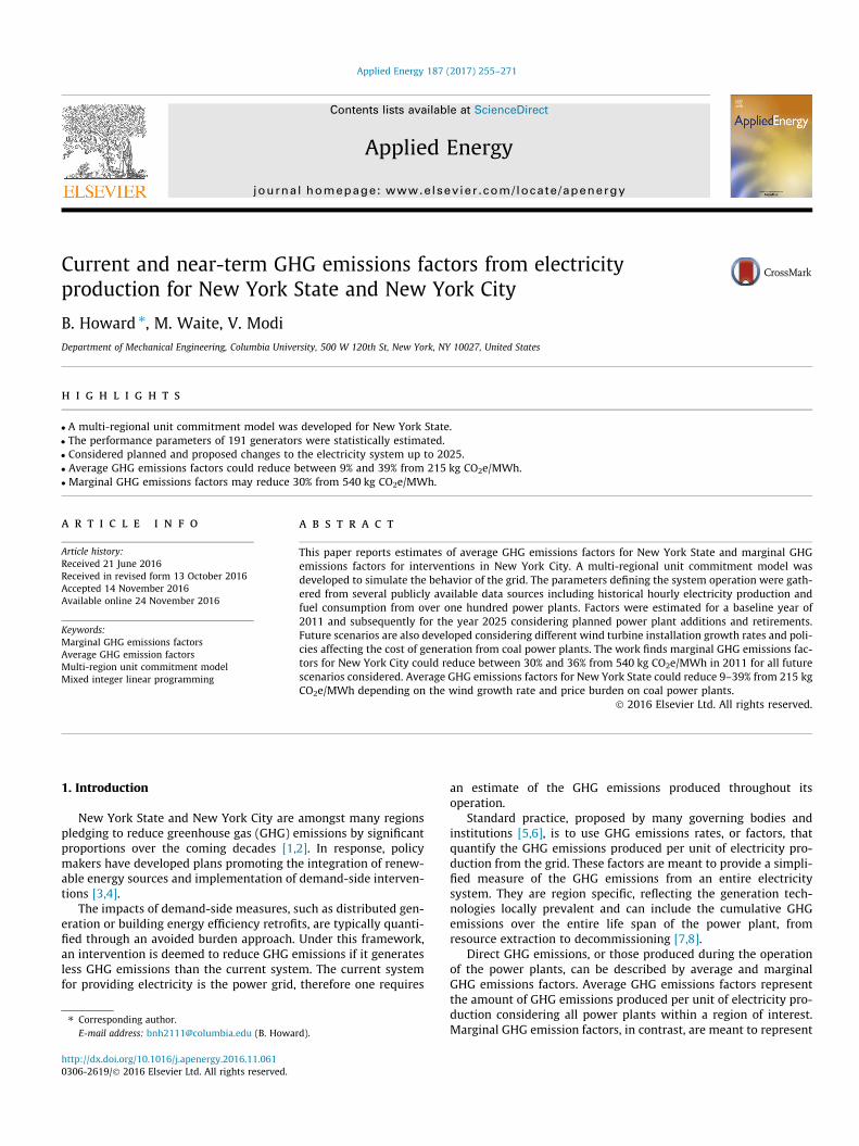
Electricity production and transmission in New York State isoverseen by the New York Independent System Operator (NYISO).NYISO divides New York State into 11 zones (labeled A through K)for the purposes of scheduling dispatch as illustrated in Fig. 1a.Zones J and K represent New York City and Long Island, respec-tively and in 2011 these demand centers contributed 47% of theannual electricity demand [23].

There are over 700 power plants in New York State included inthe markets organized by NYISO. By national standards electricityproduction in New York State is relatively low carbon with 51% ofannual electricity being provided by hydro and nuclear powerplants, 37% from natural gas (or dual fuel) sources and 7% from coalin 2011. A very small percentage (2%) of electricity generationcomes from renewable energy sources (primarily wind turbines).

In 2011, 33% of New York States annual energy demand wasfrom New York City however only 14% produced was producedwithin the City’s boundary. Therefore a significant amount of elec-

tricity is generated in the northern part of the state (upstate) andtransmitted to the southern part of the state (downstate). NewYork State also imports and exports electricity from 4 surroundingregions: PJM, the New England Independent System Operator(NEISO), Ontario’s Independent Electricity System Operator (IESO),and Hydro Quebec. In 2011, imports from these regions provided15% of the New York States electricity supply. The annual energydemand and generation by zone is depicted in Fig. 1b. Mismatchesin supply and demand as well as the significant amount of energyimported from external regions makes the transmission lines andtheir respective limits an integral aspect of power grid operation.

3. Modeling methodology

The following sections describe the multi-region unit commit-ment model used to simulate current grid operation, the methodsused to estimate average and marginal GHG emissions factors, aswell as the assumptions made for the 2025 scenarios.

3.1. Multi-region unit commitment model description

A multi-region unit commitment (MRUC) model was developedto estimate the GHG emissions produced from electricity genera-tion. A unit commitment model is an optimization problem thatdetermines the output of each power plant, or generator, withina system to minimize the overall cost of supplying demand. AMRUC model considers multiple connected regions. The connec-tions represent transmission between each region, typically apply-ing constraints reflecting power flow limits at the interface. Theoutput of the model is the fuel consumption of the generators usedto supply demand as well as the electricity flows between regions.The MRUC developed in this work does not consider the automaticdispatch of power generators for maintaining frequency and con-siders transmission across arcs as energy flows. With respect tothe time granularity considered, the commitment model usesmethods similar to those used in the day ahead market.

The MRUC model developed for New York State considers eachNYISO control zones and each import connection as a region. Theregions are connected by arcs, which represent the aggregatetransmission limits between each zone or import connection. Theformulation is similar to [24–26]. The resulting mixed-integer lin-ear program (MILP) was solved with CPLEX V12.5 [27] with theMATLAB [28] extension. The following sections will describe themathematical definitions, data sources, and limiting assumptionsfor each of the model’s components.

3.1.1. Transmission linesThe network connections between each zone include the aggre-

gate transmission limits of all 345 kV lines between each region.The aggregate lines are termed arcs and there is an upper limiton each arc. In addition to limits between regions, there are alsolimits across various interfaces. Mathematically

f a;t 6 Fþa 8a 2 A; t 2 T ð1ÞX

a2As

f a;t 6 FAs 8As 2 F ð2Þ

where f a;t is the electricity flow on arc a at time t; Fa is the maxi-

mum flow on arc, a; A is the set of all arcs, FAs is the maximumaggregate power flow of arcs in the set As

; T is the simulation timeperiod and F is the set of arcs with aggregate flow constraints. Eq.(1) describes the capacity limits on each individual arc and Eq. (2)describes aggregate limits for selected sets of arcs.

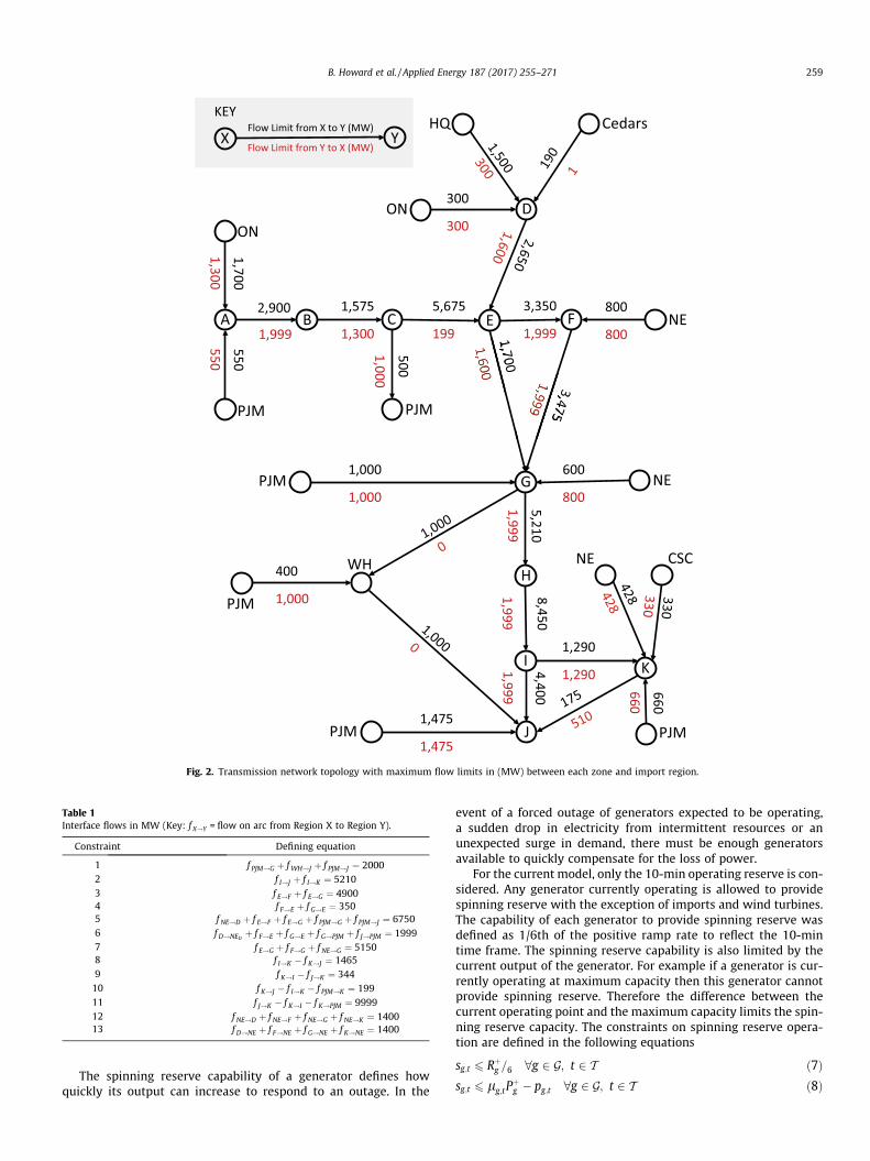
The network topology as well as the flow limits on arcs betweenzones and import regions is shown in Fig. 2. The interface limitscan be found in Table 1. As illustrated in Fig. 2, the highest limits

Fig. 1. NYISO control zones and corresponding electricity generation and demand (2011).

258 B. Howard et al. / Applied Energy 187 (2017) 255–271

on the transmission lines are in the direction of flow towards NewYork City (Zone J) and Long Island (Zone K).

3.1.2. Generator constraintsIn the formulation of the unit commitmentmodel, generators are

defined by their limiting characteristics that vary by the underlyingpower plant technology and environmental factors. However byexploring the data provided by the RGGI, these parameters can bedefined uniquely for the majority of generators in New York State.All generators are defined by the following parameters: maximumoutput, minimum output, part-load heat rate, minimum up time,minimum down time, positive and negative ramp rates, and spin-ning reserve capability. The following paragraphs describe howthese parameters were defined for each generator type. Additionalthe final parameter values can be found in the SupplementaryMaterials.

Fossil fuel power plants over 25 MW. Fossil fuel power plantsconsist of steam turbines (ST), combined cycle gas turbines (CCGT),simple cycle gas turbines (GT), internal combustion engines (ICE),and stationary jet engines (JE) fueled by natural gas, coal and fuel oil.

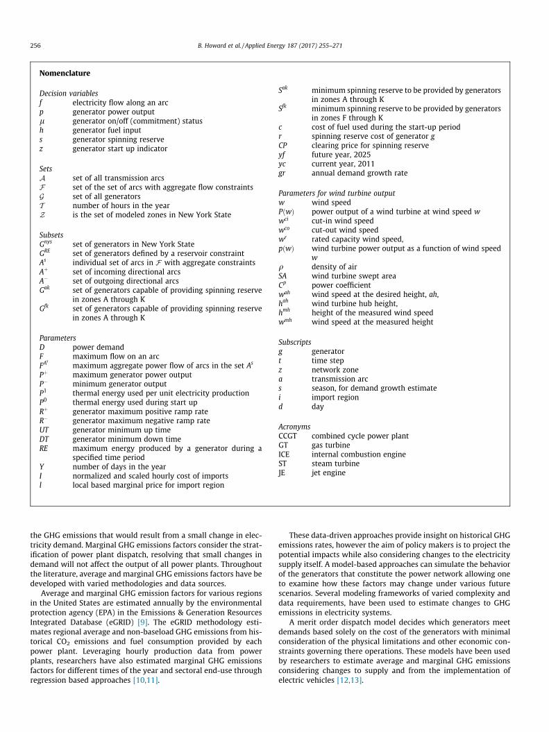
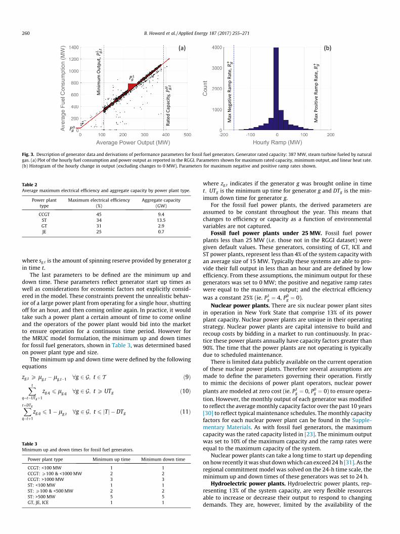
All fossil fuel power plants above 25 MW are required to reporttheir hourly fuel consumption and power output as part the Regio-nal Greenhouse Gas Initiative (RGGI) [29]. The generators coveredin this data set comprise 67% of the New York State’s power plantcapacity. Hourly data from 2011 was used to defined the minimumoutput, part-load heat rate, and ramp rates for each generator inthe set. An example of the data sets used and the derived parame-ters are shown in Fig. 3.

Fig. 3(a) depicts the fuel consumption as a function of grosspower output for a 387 MW natural gas fueled steam turbine. Alsoshown in the figure are the derived values for the maximum out-put, minimum output, linear slope of the heat rate, and interceptvalue of the heat rate.

The fuel consumption of each generator was defined as a linearfunction of the gross load as defined in the equation below

hg;t ¼ P1gpg;t þ P0

glg;t 8g 2 G; t 2 T ð3Þ

where hg;t is the fuel input in MWh of thermal energy (quantity of

fuel multiplied by the fuel content) for generator g at time t; P1g is

the thermal energy used per unit electricity production, and P0g is

the thermal energy used during start up.

For the fossil fuel generators with data reported in the RGGI, thecoefficients P1

g and P0g were found via an ordinary least squares

regression using the hourly data heat input and gross load datafrom [29]. In the literature the generator part-load efficiency isoften assumed to be a quadratic function of the load, however fromthe analysis it was found that a linear approximation providedsimilar descriptive capabilities with R2 values for all generatorsabove 0.9. Table 2 reports the average maximum electrical efficien-cies and aggregate capacity for each power plant type.

The maximum output for each fossil fuel generator, PHg;t , was

defined as the rated capacity listed for each generator listed inthe 2012 NYISO annual report [23]. The minimum output of eachfossil fuel generator was defined as the lowest 10th percentile ofall of the operating points in 2011. Overall the power limits on eachgenerator is defined as

PLglg;t 6 pg;t 6 PH

g;tlg;t 8g 2 G; t 2 T ð4Þ

where PHg;t is themaximumpower output (MW)of generator g in time

t, and PLg;t is the minimum output of generator g in time t; pg;t is the

power produced (MW) by generator g at time t; lg;t is the on/off sta-tus defined as a binary variable of the generator g in time t; G is theset of all generators, and T is the number of hours in the year.

The ramp rates define the maximum change a generator canmake in a time step. In the MRUC model, two ramp rates are used:the maximum change in power output when increasing the output(positive) and decreasing the output (negative). The positive andnegative ramp rates were defined as the maximum change experi-enced by the generator in a single hour in the respective directionover the annual 2011 data set. For the negative ramp rates, datapoints were excluded when the next time step was zero to removethe influence of generator shut downs. Fig. 3(b) depicts a histogramof thehistorical ramps rates for a single generator aswell as the eval-uated values for the maximum positive and negative ramp rates.

The mathematical constraint is described as

pg;t � pg;t�1 6 Rþg 8g 2 G; t 2 T ð5Þ

pg;t�1 � pg;t 6 R�g 8g 2 G; t 2 T ð6Þ

where Rþg is the maximum positive ramp rate of generator g, and R�

g

is the maximum negative ramp rate of generator g.

Fig. 2. Transmission network topology with maximum flow limits in (MW) between each zone and import region.

Table 1Interface flows in MW (Key: f X!Y = flow on arc from Region X to Region Y).

Constraint Defining equation

1 f PJM!G þ f WH!J þ f PJM!J ¼ 20002 f I!J þ f I!K ¼ 52103 f E!F þ f E!G ¼ 49004 f F!E þ f G!E ¼ 3505 f NE!D þ f E!F þ f E!G þ f PJM!G þ f PJM!J ¼ 67506 f D!NED þ f F!E þ f G!E þ f G!PJM þ f J!PJM ¼ 19997 f E!G þ f F!G þ f NE!G ¼ 51508 f I!K � f K!J ¼ 14659 f K!I � f J!K ¼ 34410 f K!J � f I!K � f PJM!K ¼ 19911 f J!K � f K!I � f K!PJM ¼ 999912 f NE!D þ f NE!F þ f NE!G þ f NE!K ¼ 140013 f D!NE þ f F!NE þ f G!NE þ f K!NE ¼ 1400

B. Howard et al. / Applied Energy 187 (2017) 255–271 259

The spinning reserve capability of a generator defines howquickly its output can increase to respond to an outage. In the

event of a forced outage of generators expected to be operating,a sudden drop in electricity from intermittent resources or anunexpected surge in demand, there must be enough generatorsavailable to quickly compensate for the loss of power.

For the current model, only the 10-min operating reserve is con-sidered. Any generator currently operating is allowed to providespinning reserve with the exception of imports and wind turbines.The capability of each generator to provide spinning reserve wasdefined as 1/6th of the positive ramp rate to reflect the 10-mintime frame. The spinning reserve capability is also limited by thecurrent output of the generator. For example if a generator is cur-rently operating at maximum capacity then this generator cannotprovide spinning reserve. Therefore the difference between thecurrent operating point and the maximum capacity limits the spin-ning reserve capacity. The constraints on spinning reserve opera-tion are defined in the following equations

sg;t 6 Rþg =6 8g 2 G; t 2 T ð7Þ

sg;t 6 lg;tPþg � pg;t 8g 2 G; t 2 T ð8Þ

Fig. 3. Description of generator data and derivations of performance parameters for fossil fuel generators. Generator rated capacity: 387 MW, steam turbine fueled by naturalgas. (a) Plot of the hourly fuel consumption and power output as reported in the RGGI. Parameters shown for maximum rated capacity, minimum output, and linear heat rate.(b) Histogram of the hourly change in output (excluding changes to 0 MW). Parameters for maximum negative and positive ramp rates shown.

Table 2Average maximum electrical efficiency and aggregate capacity by power plant type.

Power planttype

Maximum electrical efficiency(%)

Aggregate capacity(GW)

CCGT 45 9.4ST 34 13.5GT 31 2.9JE 25 0.7

260 B. Howard et al. / Applied Energy 187 (2017) 255–271

where sg;t is the amount of spinning reserve provided by generator gin time t.

The last parameters to be defined are the minimum up anddown time. These parameters reflect generator start up times aswell as considerations for economic factors not explicitly consid-ered in the model. These constraints prevent the unrealistic behav-ior of a large power plant from operating for a single hour, shuttingoff for an hour, and then coming online again. In practice, it wouldtake such a power plant a certain amount of time to come onlineand the operators of the power plant would bid into the marketto ensure operation for a continuous time period. However forthe MRUC model formulation, the minimum up and down timesfor fossil fuel generators, shown in Table 3, was determined basedon power plant type and size.

The minimum up and down time were defined by the followingequations

zg;t P lg;t � lg;t�1 8g 2 G; t 2 T ð9ÞXt

q¼t�UTgþ1

zg;q 6 lg;q 8g 2 G; t P UTg ð10Þ

XtþDTg

q¼tþ1

zg;q 6 1� lg;t 8g 2 G; t 6 jTj � DTg ð11Þ

Table 3Minimum up and down times for fossil fuel generators.

Power plant type Minimum up time Minimum down time

CCGT: <100 MW 1 1CCGT: P100 & <1000 MW 2 2CCGT: >1000 MW 3 3ST: <100 MW 1 1ST: P100 & <500 MW 2 2ST: >500 MW 5 5GT, JE, ICE 1 1

where zg;t indicates if the generator g was brought online in timet; UTg is the minimum up time for generator g and DTg is the min-imum down time for generator g.

For the fossil fuel power plants, the derived parameters areassumed to be constant throughout the year. This means thatchanges to efficiency or capacity as a function of environmentalvariables are not captured.

Fossil fuel power plants under 25 MW. Fossil fuel powerplants less than 25 MW (i.e. those not in the RGGI dataset) weregiven default values. These generators, consisting of GT, ICE andST power plants, represent less than 4% of the system capacity withan average size of 15 MW. Typically these systems are able to pro-vide their full output in less than an hour and are defined by lowefficiency. From these assumptions, the minimum output for thesegenerators was set to 0 MW; the positive and negative ramp rateswere equal to the maximum output; and the electrical efficiencywas a constant 25% (ie. P1

g ¼ 4, P0g ¼ 0).

Nuclear power plants. There are six nuclear power plant sitesin operation in New York State that comprise 13% of its powerplant capacity. Nuclear power plants are unique in their operatingstrategy. Nuclear power plants are capital intensive to build andrecoup costs by bidding in a market to run continuously. In prac-tice these power plants annually have capacity factors greater than90%. The time that the power plants are not operating is typicallydue to scheduled maintenance.

There is limited data publicly available on the current operationof these nuclear power plants. Therefore several assumptions aremade to define the parameters governing their operation. Firstlyto mimic the decisions of power plant operators, nuclear powerplants are modeled at zero cost (ie. P1

g ¼ 0, P0g ¼ 0) to ensure opera-

tion. However, the monthly output of each generator was modifiedto reflect the averagemonthly capacity factor over the past 10 years[30] to reflect typical maintenance schedules. Themonthly capacityfactors for each nuclear power plant can be found in the Supple-mentary Materials. As with fossil fuel generators, the maximumcapacity was the rated capacity listed in [23]. The minimum outputwas set to 10% of the maximum capacity and the ramp rates wereequal to the maximum capacity of the system.

Nuclear power plants can take a long time to start up dependingonhow recently itwas shut downwhich can exceed24 h [31]. As theregional commitment model was solved on the 24-h time scale, theminimum up and down times of these generators was set to 24 h.

Hydroelectric power plants. Hydroelectric power plants, rep-resenting 13% of the system capacity, are very flexible resourcesable to increase or decrease their output to respond to changingdemands. They are, however, limited by the availability of the

B. Howard et al. / Applied Energy 187 (2017) 255–271 261

water resource. As limited information was available on theresource availability, the hydroelectric power plants were modeledas energy reservoirs. This means that they can produce as muchpower at any given point in time, up to the rated capacity, butthe amount of energy produced over a given time period is limited;we imposed a daily energy limit. The constraint for generatorsdefined as reservoirs is as follows:

X24�dt¼24� d�1ð Þþ1

pg;t 6 REg;d 8g 2 GRE; d 2 Y ð12Þ

where REg;sti is the maximum amount of energy that can be pro-

duced by generator g in the time period sti, �h is the number of hoursin sti; GRE is the set of generators defined by a reservoir constraint,and Y is the number of consecutive time periods sti in the year.

There were 350 hydroelectric power plants in operation in2011. To reduce the model complexity, these generators wereaggregated and modeled as a single generator in each zone con-taining hydroelectric generators. This resulted in 7 aggregatehydroelectric modeled generators. The maximum output of theaggregate generators is the sum of the individual rated capacitiesof the generators within the zone.

As hydroelectric plants are flexible in their operation, the aggre-gate power plants were allowed to ramp to their full capacity andthe minimum up and down times were 1 h. As with nuclear powerplants, hydroelectric plants typically bid in themarket at low prices,therefore the plantsweremodeledwith zero cost (ie. P1

g ¼ 0, P0g ¼ 0).

The aggregate daily energy reservoir values, REg;sti , were derivedfrom the reportedmonthly output of the hydroelectric power plantswithin the zone by the EIA [30] and full list of the daily constraintscan be found in the Supplementary Materials. The spinning reservecapability was defined the same as fossil fuel generators.

Wind turbines. Wind turbines comprise of 3% the systemcapacity. The wind output of the wind sites was modeled usingwind resource estimates made by NREL and estimated powercurves for the wind turbines installed at the wind sites. The follow-ing paragraphs describe the methodology used to estimate thepower output of the 17 existing wind sites.

For each existing site data on location, number of wind turbinesat each site, wind turbine manufacturer, rated capacity powercurves, hub height, and swept area were collected and collatedfrom [32].

The power curve is a function that describes the power outputof a wind turbine given a specific wind speed. The curve is piece-wise consisting of 4 regions defined by the following equation:

PðwÞ ¼

0; if w 6 wci ð13ÞpðwÞ; if w > wci & w 6 wr ð14ÞPþ; if w > wr & w < wco ð15Þ0; if w P wco ð16Þ

8>>><>>>:

where PðwÞ is the power output of a wind turbine at wind speedw; wci is the cut-in wind speed, wr is the rated capacity wind speed,pðwÞ is the function defining the nonlinear relation between thepower output and the wind speed, Pþ is the wind turbine ratedcapacity and wco is the cut-out wind speed.

Key to defining power output of a wind turbine is defining thecurve pðwÞ. Carrillo et al. [33] tested various approximations fordeveloping continuous power curves and found that the cubicand exponential approximations provide the best fit in terms ofenergy density. Therefore for the current analysis, the cubic powercurve approximation was deemed sufficient. The cubic approxima-tion defines the power output of a wind turbine as

pðwÞ ¼ 12qðSAÞCpw3 ð17Þ

where q is the density of air, SA is wind turbine swept area, Cp is aconstant equivalent to the power coefficient, and w is the windspeed.

For each wind turbine type, five data points from the manufac-turers power curves, the reported swept area, and a constant air

density of 1:225 kg=m3 were used to estimate the value of Cp. Thisallowed for a continuous estimate of the power output. The param-eters defining the wind turbine output, i.e. rate capacity, estimatedpower coefficients, the hub heights, blade diameters, and definingwind speeds, can be found in the Supplementary Materials.

The wind resource in each location was estimated using NREL’sWind Integration Tool Kit [34]. The kit provides estimates the windresource at various sites across the Untied States including NewYork from 2007 to 2013. The selected sites are those sites that havethe potential to produce the most annual energy, considering typ-ical wind turbine power curves and buildable land area. Moredetails on the methodology of the NREL toolkit can be found in[34].

A single wind resource time series (from the year 2011) wasused for each existing wind turbine site (17 sites). The annual windresource chosen for each site was the NREL toolkit site with theclosest latitude and longitude to that of the existing wind site.The NREL model estimates winds at 100-meter hub heights how-ever the hub heights of the existing turbines were mostly at 80or 60 m. A general hub height adjustment equation

wah ¼ wmh hah

hmh

!1=7

ð18Þ

was used to adjust the wind speeds for the correct hub height. Inthe above equation, wah is the wind speed at the desired height,

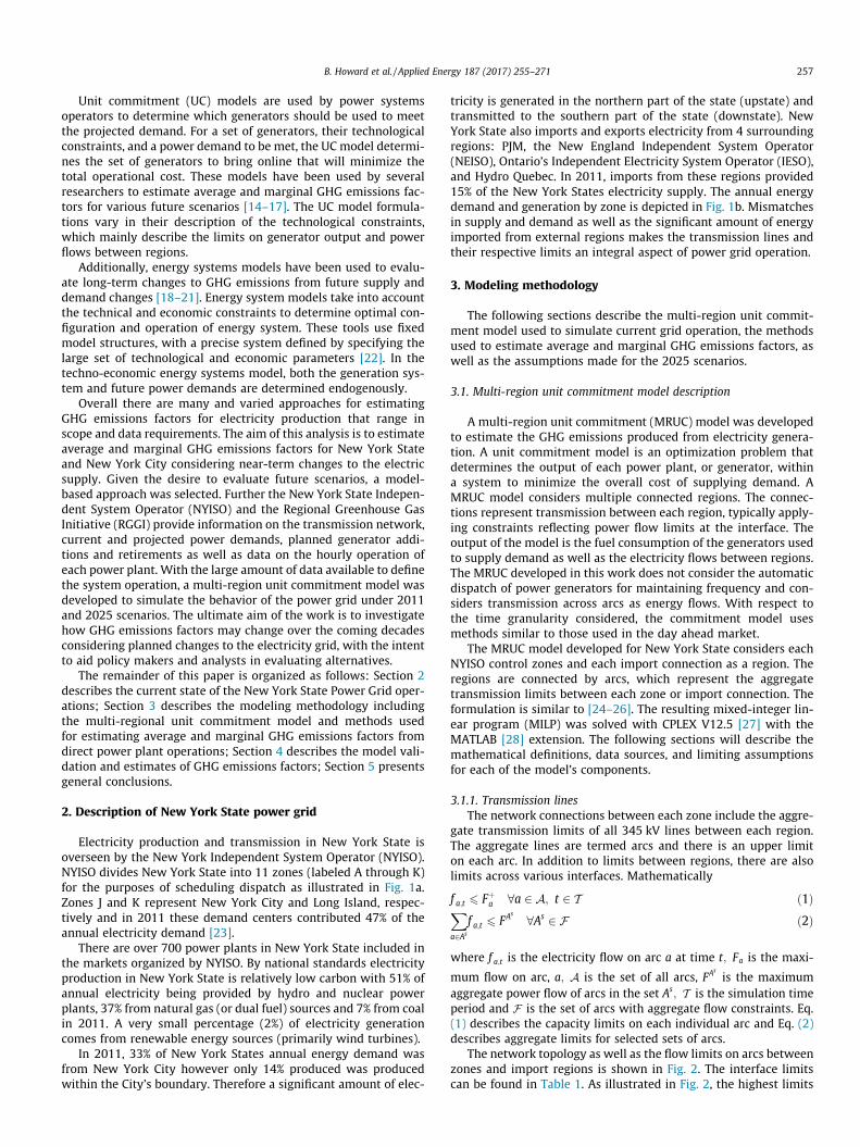
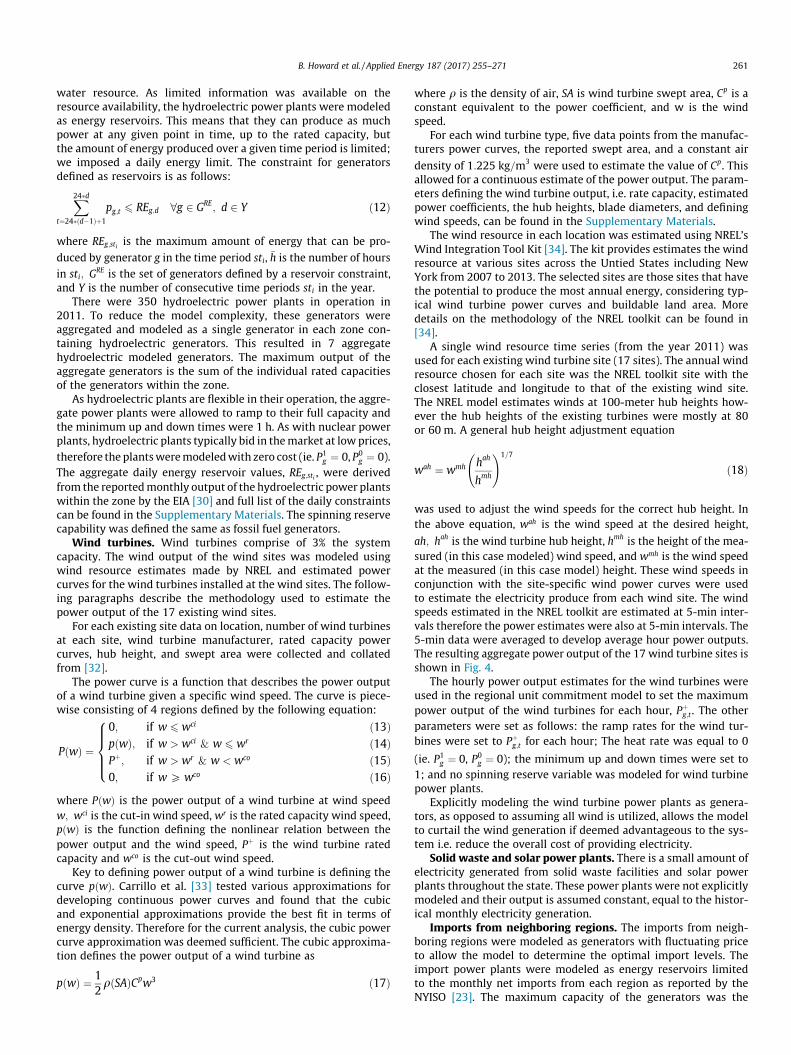
ah; hah is the wind turbine hub height, hmh is the height of the mea-sured (in this case modeled) wind speed, and wmh is the wind speedat the measured (in this case model) height. These wind speeds inconjunction with the site-specific wind power curves were usedto estimate the electricity produce from each wind site. The windspeeds estimated in the NREL toolkit are estimated at 5-min inter-vals therefore the power estimates were also at 5-min intervals. The5-min data were averaged to develop average hour power outputs.The resulting aggregate power output of the 17 wind turbine sites isshown in Fig. 4.

The hourly power output estimates for the wind turbines wereused in the regional unit commitment model to set the maximumpower output of the wind turbines for each hour, Pþ

g;t . The otherparameters were set as follows: the ramp rates for the wind tur-bines were set to Pþ

g;t for each hour; The heat rate was equal to 0

(ie. P1g ¼ 0, P0

g ¼ 0); the minimum up and down times were set to1; and no spinning reserve variable was modeled for wind turbinepower plants.

Explicitly modeling the wind turbine power plants as genera-tors, as opposed to assuming all wind is utilized, allows the modelto curtail the wind generation if deemed advantageous to the sys-tem i.e. reduce the overall cost of providing electricity.

Solid waste and solar power plants. There is a small amount ofelectricity generated from solid waste facilities and solar powerplants throughout the state. These power plants were not explicitlymodeled and their output is assumed constant, equal to the histor-ical monthly electricity generation.

Imports from neighboring regions. The imports from neigh-boring regions were modeled as generators with fluctuating priceto allow the model to determine the optimal import levels. Theimport power plants were modeled as energy reservoirs limitedto the monthly net imports from each region as reported by theNYISO [23]. The maximum capacity of the generators was the

0 1000 2000 3000 4000 5000 6000 7000 8000

Hour

0

0.5

1

1.5

Ave

rage

Pow

er O

utpu

t (G

W)

Fig. 4. Aggregate hourly power output of wind turbine sites. Total capacity: 1.4 GW.

262 B. Howard et al. / Applied Energy 187 (2017) 255–271

transmission limit of the specific import region. The minimum out-put was set to zero, the ramp rates were set equal to the maximumcapacity and the minimum up down times were 1 h. This leads toan extremely flexible resource however the hourly prices ofimports specifically shapes when imports are utilized.

Imports from neighboring regions are used to balance the sys-tem only when the price is advantageous. The price for imports,or electricity from any region, can be defined by the local basedmarginal price. The LBMP is the highest price paid for electricityfor a particular location, in this case those of the import regions.There are daily patterns, seasonal patterns, and spikes in the pricethat most likely reflect the constraints of the external systems andeffects of supply and demand. As the current model does not con-sist of a module reflecting the economics, the prices themselveswere used as basis to signal when imports should be allowed toprovide electricity.

However the LBMP for these regions are the price of electricitywhereas the other generator types are modeled to reflect the costof providing electricity. Therefore an adjustment was made toensure the imports would be competitive.

The LBMP’s for each region were normalized with the logisticsigmoid function and rescaled between the minimum and medianLBMP prices as described in the following equations

Ii;t ¼eIi;t

1þ eIi;t� ðmedðliÞ �minðliÞÞ þminðliÞ 8i 2 Z; t 2 T ð19Þ

where Ii;t is the normalized and scaled hourly cost of imports fromregion i in hour t, li is the vector the hourly LBMP for import region iin 2011, medðliÞ is the median hourly LBMP price for import region iin 2011, minðliÞ is the minimum hourly LBMP for import region i in

2011 and Ii;t is

Ii;t ¼li;t � listdðliÞ

ð20Þ

where stdðliÞ is the standard deviation of the hourly LBMP for

import region i in 2011 and li is the mean hourly LBMP for importregion i in 2011.

This normalization and rescaling retains the fluctuation in thecost based in the availably of generators in the other regions.

3.1.3. System wide constraintsThere are two system wide constraints. The first constraint dic-

tates that for each zone, the total generator output, imported andexported electricity must equal the demand in each hour, ensuring

supply meets demand at all times. This is described mathemati-cally with the following equation

XGz

g¼1

pg;t � Dz;t þXAþ

z

a¼1

f a;t �XA�

z

a¼1

f a;t ¼ 0 8z 2 Z; t 2 T ð21Þ

where Dz;t is the demand in zone z at time t; Gz is the set of gener-ators in zone z; Aþ

z is set of the arcs that follow into zone z; A�z is the

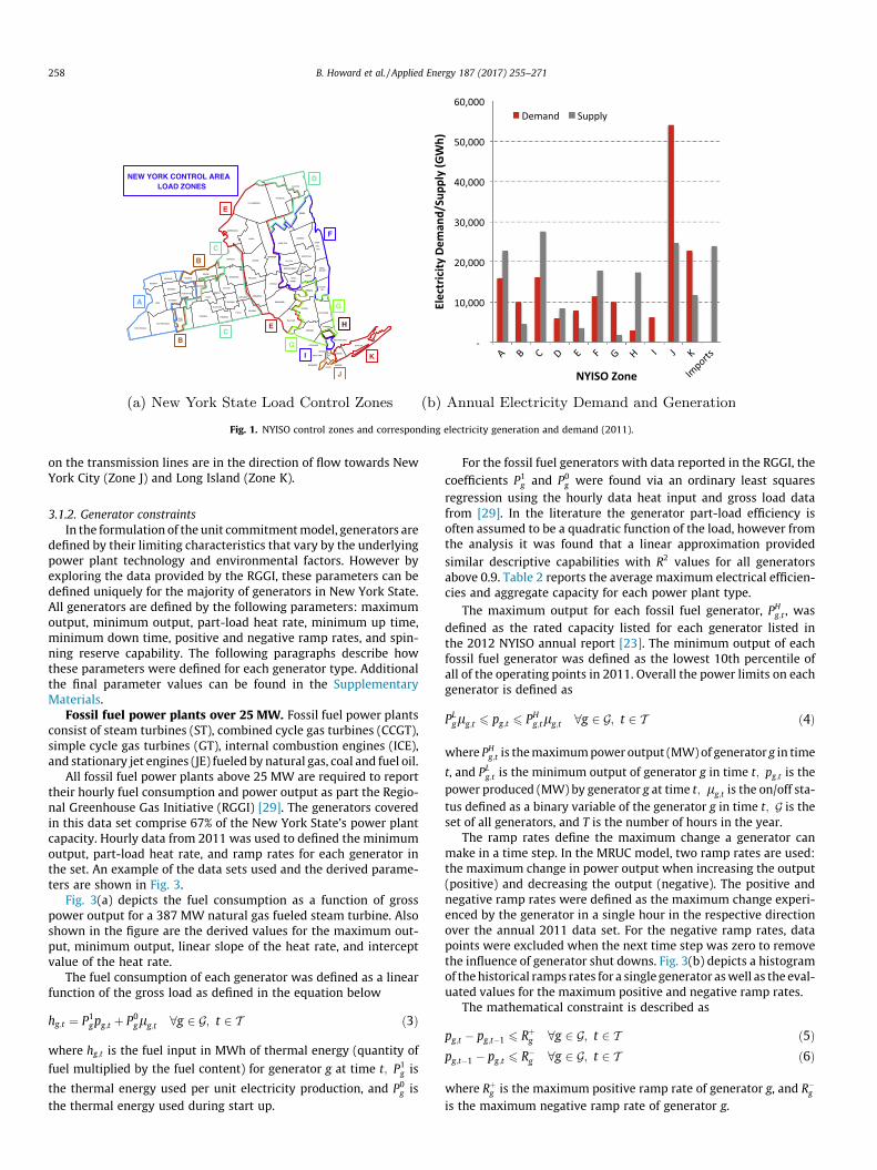
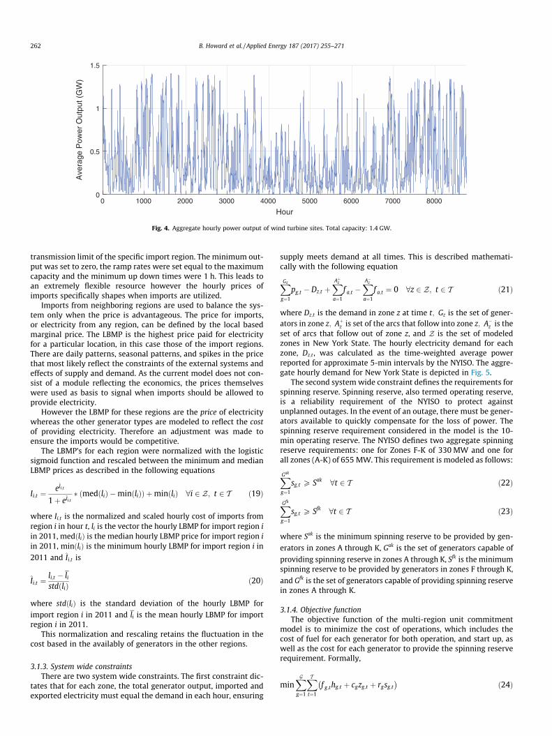
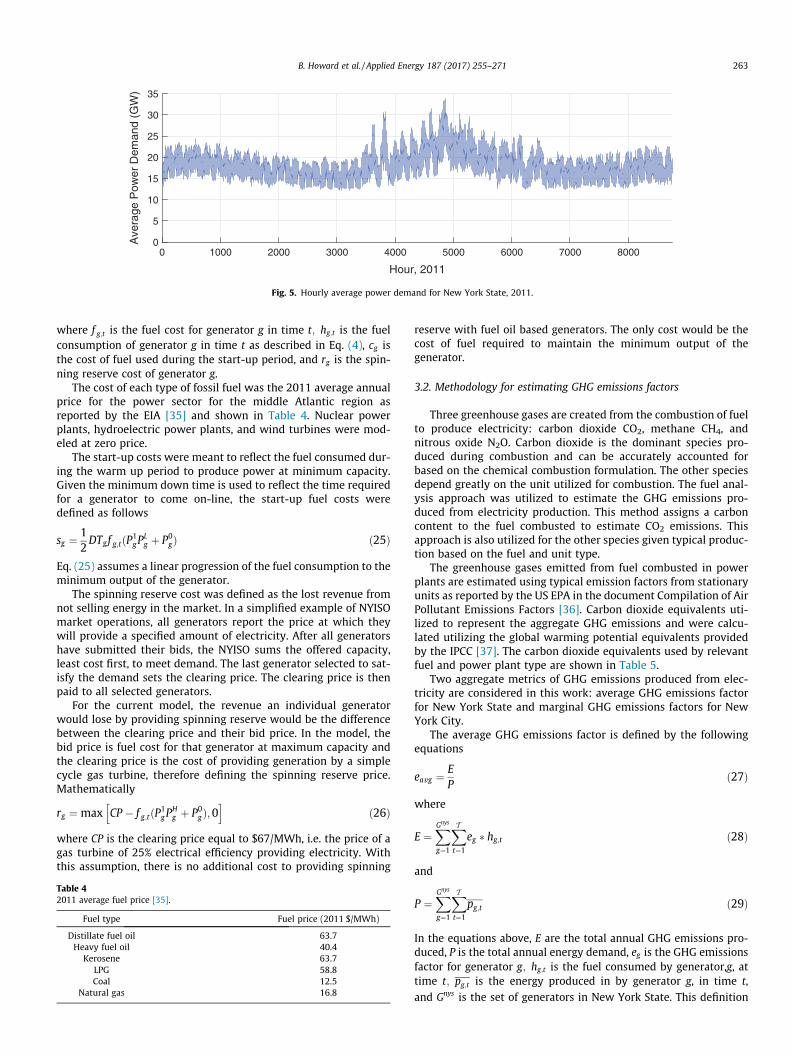
set of arcs that follow out of zone z, and Z is the set of modeledzones in New York State. The hourly electricity demand for eachzone, Dz;t , was calculated as the time-weighted average powerreported for approximate 5-min intervals by the NYISO. The aggre-gate hourly demand for New York State is depicted in Fig. 5.

The second systemwide constraint defines the requirements forspinning reserve. Spinning reserve, also termed operating reserve,is a reliability requirement of the NYISO to protect againstunplanned outages. In the event of an outage, there must be gener-ators available to quickly compensate for the loss of power. Thespinning reserve requirement considered in the model is the 10-min operating reserve. The NYISO defines two aggregate spinningreserve requirements: one for Zones F-K of 330 MW and one forall zones (A-K) of 655 MW. This requirement is modeled as follows:

XGak

g¼1

sg;t P Sak 8t 2 T ð22Þ

XGfk

g¼1

sg;t P Sfk 8t 2 T ð23Þ

where Sak is the minimum spinning reserve to be provided by gen-

erators in zones A through K, Gak is the set of generators capable of

providing spinning reserve in zones A through K, Sfk is the minimumspinning reserve to be provided by generators in zones F through K,

and Gfk is the set of generators capable of providing spinning reservein zones A through K.

3.1.4. Objective functionThe objective function of the multi-region unit commitment

model is to minimize the cost of operations, which includes thecost of fuel for each generator for both operation, and start up, aswell as the cost for each generator to provide the spinning reserverequirement. Formally,

minXGg¼1

XTt¼1

f g;thg;t þ cgzg;t þ rgsg;t� �

ð24Þ

0 1000 2000 3000 4000 5000 6000 7000 8000

Hour, 2011

0

5

10

15

20

25

30

35

Ave

rage

Pow

er D

eman

d (G

W)

Fig. 5. Hourly average power demand for New York State, 2011.

B. Howard et al. / Applied Energy 187 (2017) 255–271 263

where f g;t is the fuel cost for generator g in time t; hg;t is the fuelconsumption of generator g in time t as described in Eq. (4), cg isthe cost of fuel used during the start-up period, and rg is the spin-ning reserve cost of generator g.

The cost of each type of fossil fuel was the 2011 average annualprice for the power sector for the middle Atlantic region asreported by the EIA [35] and shown in Table 4. Nuclear powerplants, hydroelectric power plants, and wind turbines were mod-eled at zero price.

The start-up costs were meant to reflect the fuel consumed dur-ing the warm up period to produce power at minimum capacity.Given the minimum down time is used to reflect the time requiredfor a generator to come on-line, the start-up fuel costs weredefined as follows

sg ¼12DTgf g;tðP

1gP

Lg þ P0

gÞ ð25Þ

Eq. (25) assumes a linear progression of the fuel consumption to theminimum output of the generator.

The spinning reserve cost was defined as the lost revenue fromnot selling energy in the market. In a simplified example of NYISOmarket operations, all generators report the price at which theywill provide a specified amount of electricity. After all generatorshave submitted their bids, the NYISO sums the offered capacity,least cost first, to meet demand. The last generator selected to sat-isfy the demand sets the clearing price. The clearing price is thenpaid to all selected generators.

For the current model, the revenue an individual generatorwould lose by providing spinning reserve would be the differencebetween the clearing price and their bid price. In the model, thebid price is fuel cost for that generator at maximum capacity andthe clearing price is the cost of providing generation by a simplecycle gas turbine, therefore defining the spinning reserve price.Mathematically

rg ¼ max CP � f g;tðP1gP

Hg þ P0

gÞ; 0h i

ð26Þ

where CP is the clearing price equal to $67/MWh, i.e. the price of agas turbine of 25% electrical efficiency providing electricity. Withthis assumption, there is no additional cost to providing spinning

Table 42011 average fuel price [35].

Fuel type Fuel price (2011 $/MWh)

Distillate fuel oil 63.7Heavy fuel oil 40.4

Kerosene 63.7LPG 58.8Coal 12.5

Natural gas 16.8

reserve with fuel oil based generators. The only cost would be thecost of fuel required to maintain the minimum output of thegenerator.

3.2. Methodology for estimating GHG emissions factors

Three greenhouse gases are created from the combustion of fuelto produce electricity: carbon dioxide CO2, methane CH4, andnitrous oxide N2O. Carbon dioxide is the dominant species pro-duced during combustion and can be accurately accounted forbased on the chemical combustion formulation. The other speciesdepend greatly on the unit utilized for combustion. The fuel anal-ysis approach was utilized to estimate the GHG emissions pro-duced from electricity production. This method assigns a carboncontent to the fuel combusted to estimate CO2 emissions. Thisapproach is also utilized for the other species given typical produc-tion based on the fuel and unit type.

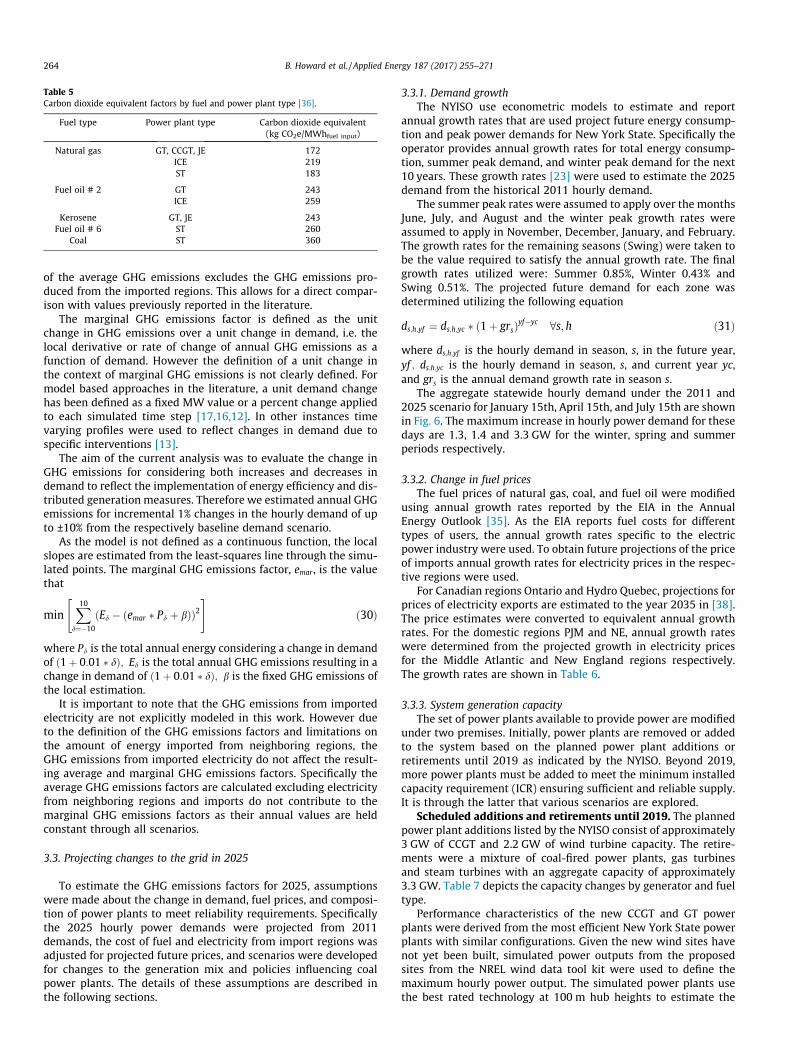
The greenhouse gases emitted from fuel combusted in powerplants are estimated using typical emission factors from stationaryunits as reported by the US EPA in the document Compilation of AirPollutant Emissions Factors [36]. Carbon dioxide equivalents uti-lized to represent the aggregate GHG emissions and were calcu-lated utilizing the global warming potential equivalents providedby the IPCC [37]. The carbon dioxide equivalents used by relevantfuel and power plant type are shown in Table 5.

Two aggregate metrics of GHG emissions produced from elec-tricity are considered in this work: average GHG emissions factorfor New York State and marginal GHG emissions factors for NewYork City.

The average GHG emissions factor is defined by the followingequations

eavg ¼EP

ð27Þ

where

E ¼XGnys

g¼1

XTt¼1

eg � hg;t ð28Þ

and

P ¼XGnys

g¼1

XTt¼1

pg;t ð29Þ

In the equations above, E are the total annual GHG emissions pro-duced, P is the total annual energy demand, eg is the GHG emissionsfactor for generator g; hg;t is the fuel consumed by generator,g, attime t; pg;t is the energy produced in by generator g, in time t,and Gnys is the set of generators in New York State. This definition

Table 5Carbon dioxide equivalent factors by fuel and power plant type [36].

Fuel type Power plant type Carbon dioxide equivalent(kg CO2e/MWhfuel input)

Natural gas GT, CCGT, JE 172ICE 219ST 183

Fuel oil # 2 GT 243ICE 259

Kerosene GT, JE 243Fuel oil # 6 ST 260

Coal ST 360

264 B. Howard et al. / Applied Energy 187 (2017) 255–271

of the average GHG emissions excludes the GHG emissions pro-duced from the imported regions. This allows for a direct compar-ison with values previously reported in the literature.

The marginal GHG emissions factor is defined as the unitchange in GHG emissions over a unit change in demand, i.e. thelocal derivative or rate of change of annual GHG emissions as afunction of demand. However the definition of a unit change inthe context of marginal GHG emissions is not clearly defined. Formodel based approaches in the literature, a unit demand changehas been defined as a fixed MW value or a percent change appliedto each simulated time step [17,16,12]. In other instances timevarying profiles were used to reflect changes in demand due tospecific interventions [13].

The aim of the current analysis was to evaluate the change inGHG emissions for considering both increases and decreases indemand to reflect the implementation of energy efficiency and dis-tributed generation measures. Therefore we estimated annual GHGemissions for incremental 1% changes in the hourly demand of upto ±10% from the respectively baseline demand scenario.

As the model is not defined as a continuous function, the localslopes are estimated from the least-squares line through the simu-lated points. The marginal GHG emissions factor, emar , is the valuethat

minX10d¼�10

Ed � ðemar � Pd þ bÞð Þ2" #

ð30Þ

where Pd is the total annual energy considering a change in demandof ð1þ 0:01 � dÞ; Ed is the total annual GHG emissions resulting in achange in demand of ð1þ 0:01 � dÞ; b is the fixed GHG emissions ofthe local estimation.

It is important to note that the GHG emissions from importedelectricity are not explicitly modeled in this work. However dueto the definition of the GHG emissions factors and limitations onthe amount of energy imported from neighboring regions, theGHG emissions from imported electricity do not affect the result-ing average and marginal GHG emissions factors. Specifically theaverage GHG emissions factors are calculated excluding electricityfrom neighboring regions and imports do not contribute to themarginal GHG emissions factors as their annual values are heldconstant through all scenarios.

3.3. Projecting changes to the grid in 2025

To estimate the GHG emissions factors for 2025, assumptionswere made about the change in demand, fuel prices, and composi-tion of power plants to meet reliability requirements. Specificallythe 2025 hourly power demands were projected from 2011demands, the cost of fuel and electricity from import regions wasadjusted for projected future prices, and scenarios were developedfor changes to the generation mix and policies influencing coalpower plants. The details of these assumptions are described inthe following sections.

3.3.1. Demand growthThe NYISO use econometric models to estimate and report

annual growth rates that are used project future energy consump-tion and peak power demands for New York State. Specifically theoperator provides annual growth rates for total energy consump-tion, summer peak demand, and winter peak demand for the next10 years. These growth rates [23] were used to estimate the 2025demand from the historical 2011 hourly demand.

The summer peak rates were assumed to apply over the monthsJune, July, and August and the winter peak growth rates wereassumed to apply in November, December, January, and February.The growth rates for the remaining seasons (Swing) were taken tobe the value required to satisfy the annual growth rate. The finalgrowth rates utilized were: Summer 0.85%, Winter 0.43% andSwing 0.51%. The projected future demand for each zone wasdetermined utilizing the following equation

ds;h;yf ¼ ds;h;yc � ð1þ grsÞyf�yc 8s; h ð31Þ

where ds;h;yf is the hourly demand in season, s, in the future year,yf ; ds;h;yc is the hourly demand in season, s, and current year yc,and grs is the annual demand growth rate in season s.

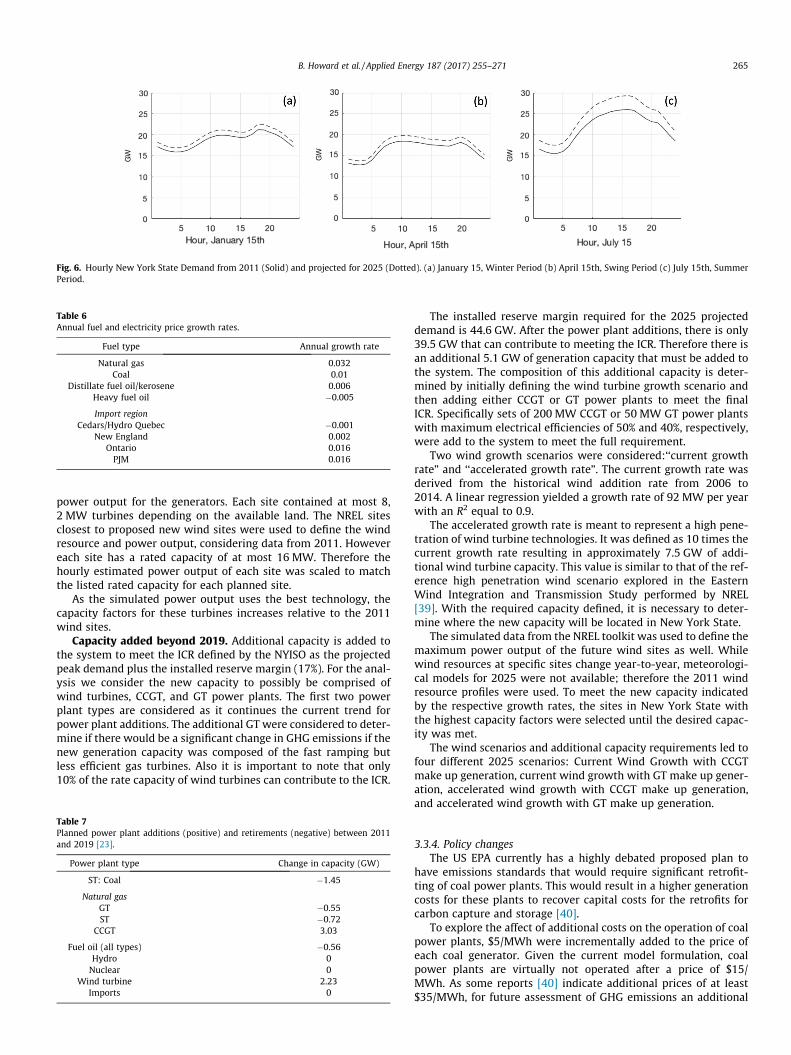
The aggregate statewide hourly demand under the 2011 and2025 scenario for January 15th, April 15th, and July 15th are shownin Fig. 6. The maximum increase in hourly power demand for thesedays are 1.3, 1.4 and 3.3 GW for the winter, spring and summerperiods respectively.

3.3.2. Change in fuel pricesThe fuel prices of natural gas, coal, and fuel oil were modified

using annual growth rates reported by the EIA in the AnnualEnergy Outlook [35]. As the EIA reports fuel costs for differenttypes of users, the annual growth rates specific to the electricpower industry were used. To obtain future projections of the priceof imports annual growth rates for electricity prices in the respec-tive regions were used.

For Canadian regions Ontario and Hydro Quebec, projections forprices of electricity exports are estimated to the year 2035 in [38].The price estimates were converted to equivalent annual growthrates. For the domestic regions PJM and NE, annual growth rateswere determined from the projected growth in electricity pricesfor the Middle Atlantic and New England regions respectively.The growth rates are shown in Table 6.

3.3.3. System generation capacityThe set of power plants available to provide power are modified

under two premises. Initially, power plants are removed or addedto the system based on the planned power plant additions orretirements until 2019 as indicated by the NYISO. Beyond 2019,more power plants must be added to meet the minimum installedcapacity requirement (ICR) ensuring sufficient and reliable supply.It is through the latter that various scenarios are explored.

Scheduled additions and retirements until 2019. The plannedpower plant additions listed by the NYISO consist of approximately3 GW of CCGT and 2.2 GW of wind turbine capacity. The retire-ments were a mixture of coal-fired power plants, gas turbinesand steam turbines with an aggregate capacity of approximately3.3 GW. Table 7 depicts the capacity changes by generator and fueltype.

Performance characteristics of the new CCGT and GT powerplants were derived from the most efficient New York State powerplants with similar configurations. Given the new wind sites havenot yet been built, simulated power outputs from the proposedsites from the NREL wind data tool kit were used to define themaximum hourly power output. The simulated power plants usethe best rated technology at 100 m hub heights to estimate the

Fig. 6. Hourly New York State Demand from 2011 (Solid) and projected for 2025 (Dotted). (a) January 15, Winter Period (b) April 15th, Swing Period (c) July 15th, SummerPeriod.

Table 6Annual fuel and electricity price growth rates.

Fuel type Annual growth rate

Natural gas 0.032Coal 0.01

Distillate fuel oil/kerosene 0.006Heavy fuel oil �0.005

Import regionCedars/Hydro Quebec �0.001

New England 0.002Ontario 0.016PJM 0.016

B. Howard et al. / Applied Energy 187 (2017) 255–271 265

power output for the generators. Each site contained at most 8,2 MW turbines depending on the available land. The NREL sitesclosest to proposed new wind sites were used to define the windresource and power output, considering data from 2011. Howevereach site has a rated capacity of at most 16 MW. Therefore thehourly estimated power output of each site was scaled to matchthe listed rated capacity for each planned site.

As the simulated power output uses the best technology, thecapacity factors for these turbines increases relative to the 2011wind sites.

Capacity added beyond 2019. Additional capacity is added tothe system to meet the ICR defined by the NYISO as the projectedpeak demand plus the installed reserve margin (17%). For the anal-ysis we consider the new capacity to possibly be comprised ofwind turbines, CCGT, and GT power plants. The first two powerplant types are considered as it continues the current trend forpower plant additions. The additional GT were considered to deter-mine if there would be a significant change in GHG emissions if thenew generation capacity was composed of the fast ramping butless efficient gas turbines. Also it is important to note that only10% of the rate capacity of wind turbines can contribute to the ICR.

Table 7Planned power plant additions (positive) and retirements (negative) between 2011and 2019 [23].

Power plant type Change in capacity (GW)

ST: Coal �1.45

Natural gasGT �0.55ST �0.72

CCGT 3.03

Fuel oil (all types) �0.56Hydro 0Nuclear 0

Wind turbine 2.23Imports 0

The installed reserve margin required for the 2025 projecteddemand is 44.6 GW. After the power plant additions, there is only39.5 GW that can contribute to meeting the ICR. Therefore there isan additional 5.1 GW of generation capacity that must be added tothe system. The composition of this additional capacity is deter-mined by initially defining the wind turbine growth scenario andthen adding either CCGT or GT power plants to meet the finalICR. Specifically sets of 200 MW CCGT or 50 MW GT power plantswith maximum electrical efficiencies of 50% and 40%, respectively,were add to the system to meet the full requirement.

Two wind growth scenarios were considered:‘‘current growthrate” and ‘‘accelerated growth rate”. The current growth rate wasderived from the historical wind addition rate from 2006 to2014. A linear regression yielded a growth rate of 92 MW per yearwith an R2 equal to 0.9.

The accelerated growth rate is meant to represent a high pene-tration of wind turbine technologies. It was defined as 10 times thecurrent growth rate resulting in approximately 7.5 GW of addi-tional wind turbine capacity. This value is similar to that of the ref-erence high penetration wind scenario explored in the EasternWind Integration and Transmission Study performed by NREL[39]. With the required capacity defined, it is necessary to deter-mine where the new capacity will be located in New York State.

The simulated data from the NREL toolkit was used to define themaximum power output of the future wind sites as well. Whilewind resources at specific sites change year-to-year, meteorologi-cal models for 2025 were not available; therefore the 2011 windresource profiles were used. To meet the new capacity indicatedby the respective growth rates, the sites in New York State withthe highest capacity factors were selected until the desired capac-ity was met.

The wind scenarios and additional capacity requirements led tofour different 2025 scenarios: Current Wind Growth with CCGTmake up generation, current wind growth with GT make up gener-ation, accelerated wind growth with CCGT make up generation,and accelerated wind growth with GT make up generation.

3.3.4. Policy changesThe US EPA currently has a highly debated proposed plan to

have emissions standards that would require significant retrofit-ting of coal power plants. This would result in a higher generationcosts for these plants to recover capital costs for the retrofits forcarbon capture and storage [40].

To explore the affect of additional costs on the operation of coalpower plants, $5/MWh were incrementally added to the price ofeach coal generator. Given the current model formulation, coalpower plants are virtually not operated after a price of $15/MWh. As some reports [40] indicate additional prices of at least$35/MWh, for future assessment of GHG emissions an additional

266 B. Howard et al. / Applied Energy 187 (2017) 255–271

scenario of a coal price of $35/MWh was utilized to provide insightto a scenario where there is a cost burden on coal power plants.

3.3.5. Transmission upgradesThe aim of this analysis is to evaluate the impacts of near term

changes on the GHG emissions from electricity production. Trans-mission lines represent a defining characteristics of the electricitysystem. However according to the NYISO [23], there are no signif-icant planned upgrades to the transmission lines in the comingyears. Therefore for the future scenarios, the transmissions con-straints remain the same as in the 2011 case.

4. Results and discussion

In the following sections, the validation of the MRUC model,2011 marginal GHG emissions factors, and GHG emissions factorsfor 2025 scenarios are discussed.

4.1. Model validation

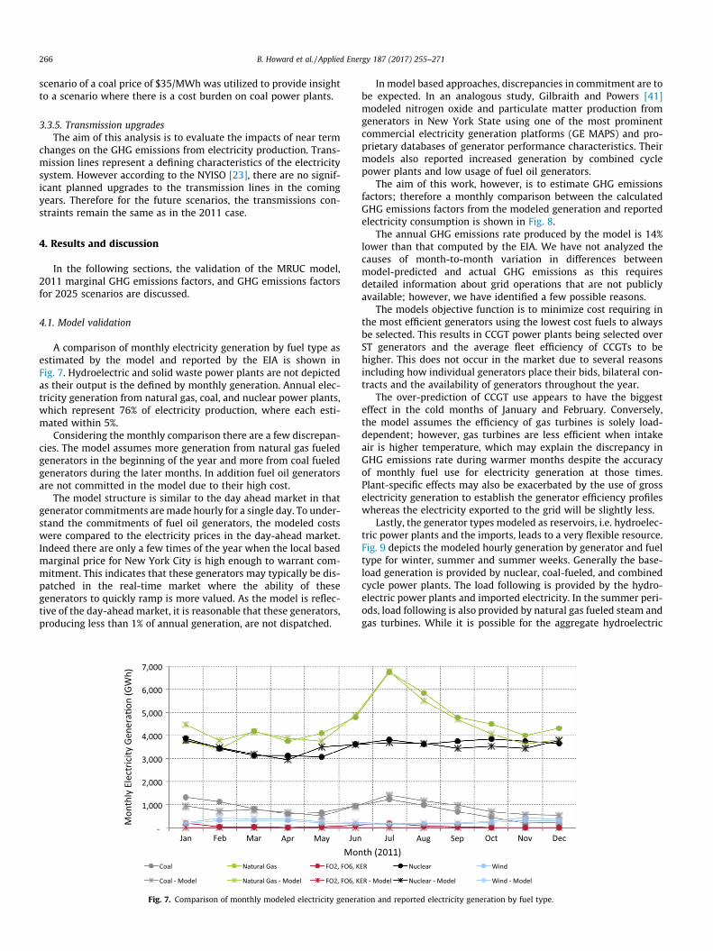
A comparison of monthly electricity generation by fuel type asestimated by the model and reported by the EIA is shown inFig. 7. Hydroelectric and solid waste power plants are not depictedas their output is the defined by monthly generation. Annual elec-tricity generation from natural gas, coal, and nuclear power plants,which represent 76% of electricity production, where each esti-mated within 5%.

Considering the monthly comparison there are a few discrepan-cies. The model assumes more generation from natural gas fueledgenerators in the beginning of the year and more from coal fueledgenerators during the later months. In addition fuel oil generatorsare not committed in the model due to their high cost.

The model structure is similar to the day ahead market in thatgenerator commitments aremade hourly for a single day. To under-stand the commitments of fuel oil generators, the modeled costswere compared to the electricity prices in the day-ahead market.Indeed there are only a few times of the year when the local basedmarginal price for New York City is high enough to warrant com-mitment. This indicates that these generators may typically be dis-patched in the real-time market where the ability of thesegenerators to quickly ramp is more valued. As the model is reflec-tive of the day-ahead market, it is reasonable that these generators,producing less than 1% of annual generation, are not dispatched.

Fig. 7. Comparison of monthly modeled electricity genera

In model based approaches, discrepancies in commitment are tobe expected. In an analogous study, Gilbraith and Powers [41]modeled nitrogen oxide and particulate matter production fromgenerators in New York State using one of the most prominentcommercial electricity generation platforms (GE MAPS) and pro-prietary databases of generator performance characteristics. Theirmodels also reported increased generation by combined cyclepower plants and low usage of fuel oil generators.

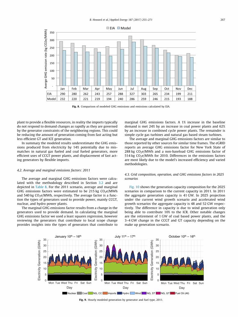
The aim of this work, however, is to estimate GHG emissionsfactors; therefore a monthly comparison between the calculatedGHG emissions factors from the modeled generation and reportedelectricity consumption is shown in Fig. 8.

The annual GHG emissions rate produced by the model is 14%lower than that computed by the EIA. We have not analyzed thecauses of month-to-month variation in differences betweenmodel-predicted and actual GHG emissions as this requiresdetailed information about grid operations that are not publiclyavailable; however, we have identified a few possible reasons.

The models objective function is to minimize cost requiring inthe most efficient generators using the lowest cost fuels to alwaysbe selected. This results in CCGT power plants being selected overST generators and the average fleet efficiency of CCGTs to behigher. This does not occur in the market due to several reasonsincluding how individual generators place their bids, bilateral con-tracts and the availability of generators throughout the year.

The over-prediction of CCGT use appears to have the biggesteffect in the cold months of January and February. Conversely,the model assumes the efficiency of gas turbines is solely load-dependent; however, gas turbines are less efficient when intakeair is higher temperature, which may explain the discrepancy inGHG emissions rate during warmer months despite the accuracyof monthly fuel use for electricity generation at those times.Plant-specific effects may also be exacerbated by the use of grosselectricity generation to establish the generator efficiency profileswhereas the electricity exported to the grid will be slightly less.

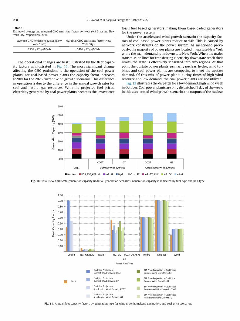
Lastly, the generator types modeled as reservoirs, i.e. hydroelec-tric power plants and the imports, leads to a very flexible resource.Fig. 9 depicts the modeled hourly generation by generator and fueltype for winter, summer and summer weeks. Generally the base-load generation is provided by nuclear, coal-fueled, and combinedcycle power plants. The load following is provided by the hydro-electric power plants and imported electricity. In the summer peri-ods, load following is also provided by natural gas fueled steam andgas turbines. While it is possible for the aggregate hydroelectric

tion and reported electricity generation by fuel type.

Fig. 8. Comparison of modeled GHG emissions and emissions calculated by EIA.

B. Howard et al. / Applied Energy 187 (2017) 255–271 267

plant to provide a flexible resources, in reality the imports typicallydo not respond to demand changes as rapidly as they are governedby the generator constraints of the neighboring regions. This couldbe reducing the amount of generation coming from fast acting butless efficient GT and ICE generation.

In summary the modeled results underestimate the GHG emis-sions produced from electricity by 14% potentially due to mis-matches in natural gas fueled and coal fueled generators, moreefficient uses of CCGT power plants, and displacement of fast act-ing generators by flexible imports.

4.2. Average and marginal emissions factors: 2011

The average and marginal GHG emissions factors were calcu-lated with the methodology described in Section 3.2 and aredepicted in Table 8. For the 2011 scenario, average and marginalGHG emissions factors were estimated to be 215 kg CO2e/MWhand 540 kg CO2e/MWh, respectively. The average factor is a func-tion the types of generators used to provide power, mainly CCGT,nuclear, and hydro power plants.

The marginal GHG emissions factor results from a change in thegenerators used to provide demand. In calculating the marginalGHG emissions factor we used a least squares regression, howeverreviewing the generators that contribute to local scope changeprovides insights into the types of generators that contribute to

Mon Tue Wed Thu Fri Sat Sun

Day

0

5

10

15

20

25

30

35

Ele

ctric

ity G

ener

atio

n (G

Wh)

D

0

5

10

15

20

25

30

35

Ele

ctric

ity G

ener

atio

n (G

Wh)

Nuclear Coal NG, CC Imports H

January 10th th July 11

Mon Tue Wed

Fig. 9. Hourly modeled generation b

marginal GHG emissions factors. A 1% increase in the baselinedemand is met 24% by an increase in coal power plants and 62%by an increase in combined cycle power plants. The remainder issimple cycle gas turbines and natural gas based steam turbines.

The average and marginal GHG emissions factors are similar tothose reported by other sources for similar time frames. The eGRIDreports an average GHG emissions factor for New York State of288 kg CO2e/MWh and a non-baseload GHG emissions factor of514 kg CO2e/MWh for 2010. Differences in the emissions factorsare most likely due to the model’s increased efficiency and variedmethodologies.

4.3. Grid composition, operation, and GHG emissions factors in 2025scenarios

Fig. 10 shows the generation capacity composition for the 2025scenarios in comparison to the current capacity in 2011. In 2011the aggregate generation capacity is 41 GW. In 2025 projectionunder the current wind growth scenario and accelerated windgrowth scenarios the aggregate capacity is 48 and 52 GW respec-tively. The difference in capacity is due to wind generation onlybeing able to contribute 10% to the ICR. Other notable changesare the retirement of 1 GW of coal based power plants, and the3–4 GW change in the CCGT and GT capacity depending on themake up generation scenario.

ay Day

0

5

10

15

20

25

30

35

Ele

ctric

ity G

ener

atio

n (G

Wh)

ydro Wind NG, ST NG, GT Fuel Oil (All)

th th October 10th th

Thu Fri Sat Sun Mon Tue Wed Thu Fri Sat Sun

y generator and fuel type, 2011.

Table 8Estimated average and marginal GHG emissions factors for New York State and NewYork City, respectively, 2011.

Average GHG emissions factor (NewYork State)

Marginal GHG emissions factor (NewYork City)

215 kg CO2e/MWh 540 kg CO2e/MWh

268 B. Howard et al. / Applied Energy 187 (2017) 255–271

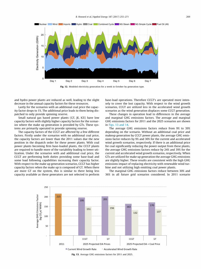
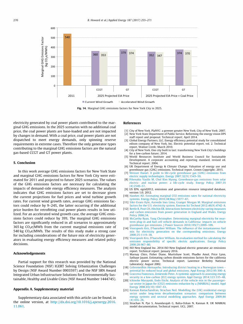
The operational changes are best illustrated by the fleet capac-ity factors as illustrated in Fig. 11. The most significant changeaffecting the GHG emissions is the operation of the coal powerplants. For coal-based power plants the capacity factor increasesto 90% for the 2025 current wind growth scenarios. This differencein operation is due to the difference in the annual growth rates forcoal and natural gas resources. With the projected fuel prices,electricity generated by coal power plants becomes the lowest cost

Fig. 11. Annual fleet capacity factors by generation type for w

Fig. 10. Total New York State generation capacity under all generation sc

fossil fuel based generators making them base-loaded generatorsfor the power system.

Under the accelerated wind growth scenario the capacity fac-tors of coal based power plants reduce to 54%. This is caused bynetwork constraints on the power system. As mentioned previ-ously, the majority of power plants are located in upstate New Yorkwhile the main demand is in downstate New York. When the majortransmission lines for transferring electricity downstate reach theirlimits, the state is effectively separated into two regions. At thatpoint the upstate power plants, primarily nuclear, hydro, wind tur-bines and coal power plants, are competing to meet the upstatedemand. Of this mix of power plants during times of high windresource and low demand, the coal power plants are not utilized.

Fig. 12 illustrates the dispatch for a low demand, highwindweekin October. Coal power plants are only dispatched 1 day of theweek.In this accelerated wind growth scenario, the outputs of the nuclear

ind growth, makeup generation, and coal price scenarios.

enarios. Generation capacity is indicated by fuel type and unit type.

Day 1 Day 2 Day 3 Day 4 Day 5 Day 6 Day 70

5

10

15

20E

lect

ricity

Gen

erat

ion

(GW

h)

Nuclear Wind Imports Hydro Coal Combined Cycle NG Steam NG Simple Cycle Fuel Oil (All)

Fig. 12. Modeled electricity generation for a week in October by generation type.

B. Howard et al. / Applied Energy 187 (2017) 255–271 269

and hydro power plants are reduced as well, leading to the slightdecrease in the annual capacity factors for these resources.

Lastly for the scenarios with an additional coal price the capac-ity factor drops to 1%. The additional price leads to them being dis-patched to only provide spinning reserve.

Small natural gas based power plants (GT, JE, ICE) have lowcapacity factors with slightly higher capacity factors for the scenar-ios where the make up generation is provided by GTs. These sys-tems are primarily operated to provide spinning reserve.

The capacity factors of the CCGT are affected by a few differentfactors. Firstly under the scenarios with no additional coal price,the capacity factors are lower than the 2011 values due the newposition in the dispatch order for these power plants. With coalpower plants becoming firm base-loaded plants, the CCGT plantsare required to handle more of the variability leading to lower uti-lization. Under the scenarios with and additional coal price, theCCGT are performing both duties providing some base-load andsome load following capabilities increasing their capacity factor.With respect to the make up generation scenarios, CCGT has highercapacity factors when the make up is composed of GT. When thereare more GT on the system, this is similar to there being lesscapacity available as these generators are not selected to perform

Fig. 13. Average GHG emissions

base-load operations. Therefore CCGT’s are operated more inten-sely to cover the lost capacity. With respect to the wind growthscenarios, CCGT are utilized less in the accelerated wind growthscenarios as the wind generation displaces some CCGT generation.

These changes in operation lead to differences in the averageand marginal GHG emissions factors. The average and marginalGHG emissions factors for 2011 and the 2025 scenarios are shownin Figs. 13 and 14.

The average GHG emissions factors reduce from 9% to 39%depending on the scenario. Without an additional coal price andmakeup generation by CCGT power plants, the average GHG emis-sions factor reduces by 9% and 30% for the current and acceleratedwind growth scenarios, respectively. If there is an additional pricefor coal significantly reducing the power output from these plants,the average GHG emissions factors reduce by 24% and 39% for thecurrent and accelerated wind growth scenarios, respectively. WhenGTs are utilized for make up generation the average GHG emissionsare slightly higher. These results are consistent with the high GHGemissions impact of replacing electricity with renewable wind tur-bine and not utilizing high emitting coal power plants.

The marginal GHG emissions factors reduce between 30% and36% in all future grid scenarios considered. In 2011 scenario

factors for 2011 and 2025.

Fig. 14. Marginal GHG emissions factors for New York City in 2025.

270 B. Howard et al. / Applied Energy 187 (2017) 255–271

electricity generated by coal power plants contributed to the mar-ginal GHG emissions. In the 2025 scenarios with no additional coalprice, the coal power plants are base-loaded and are not impactedby changes in demand. With a coal price, coal power plants are notdispatched to meet energy demands, only spinning reserverequirements in extreme cases. Therefore the only generator typescontributing to the marginal GHG emissions factors are the naturalgas-based CCGT and GT power plants.

5. Conclusion

In this work average GHG emissions factors for New York Stateand marginal GHG emissions factors for New York City were esti-mated for 2011 and projected to future 2025 scenarios. The valuesof the GHG emissions factors are necessary for calculating theimpacts of demand-side energy efficiency measures. The analysisindicates that GHG emissions factors are set to decrease giventhe current projections for fuel prices and wind turbine growthrates. For current wind growth rates, average GHG emissions fac-tors could reduce by 9–24%, the latter occurring if the additionalprice burden for retrofitting coal power plants results in low uti-lized. For an accelerated wind growth case, the average GHG emis-sions factors could reduce by 39%. The marginal GHG emissionsfactors are significantly reduced in all scenarios to approximately365 kg CO2e/MWh from the current marginal emissions rate of540 kg CO2e/MWh. The results of this study make a strong casefor including considerations of the future mix of electricity gener-ators in evaluating energy efficiency measures and related policydecisions.

Acknowledgements

Partial support for this research was provided by the NationalScience Foundation (NSF) IGERT Solving Urbanization Challengesby Design (NSF Award Number 0903597) and the NSF SRN AwardIntegrated Urban Infrastructure Solutions for Environmentally Sus-tainable, Healthy and Livable Cities (NSF Award Number 1444745).

Appendix A. Supplementary material

Supplementary data associated with this article can be found, inthe online version, at http://dx.doi.org/10.1016/j.apenergy.2016.11.061.

References

[1] City of New York. PlaNYC: a greener greater New York. City of New York; 2007.[2] New York State Department of Public Service. Reforming the energy vision DPS

staff report and proposal. Technical report; April 2014.[3] Global Energy Partners, LLC. Energy efficiency potential study for consolidated

edison company of New York, Inc. Electric potential report, vol. 2. Technicalreport. Walnut Creek; March 2010.

[4] City of New York. One city built to last: transforming New York City’s buildingsfor a low-carbon future; 2014.

[5] World Resources Institute and World Business Council for SustainableDevelopment. A corporate accounting and reporting standard. revised ed.Technical report; 2004.

[6] UK Department of Energy & Climate Change. Valuation of energy use andgreenhouse gas (GHG) emissions. Technical report. Crown Copyright; 2015.

[7] Weisser Daniel. A guide to life-cycle greenhouse gas (GHG) emissions fromelectric supply technologies. Energy 2007;32(9):1543–59.

[8] Fthenakis Vasilis M, Chul Kim Hyung. Greenhouse-gas emissions from solarelectric- and nuclear power: a life-cycle study. Energy Policy 2007;35(4):2549–57.

[9] US EPA. egrid2012, emissions and generation resource integrated database,version 1.0; 2012.

[10] Hawkes AD. Estimating marginal CO2 emissions rates for national electricitysystems. Energy Policy 2010;38(May):5977–87.

[11] Siler-Evans Kyle, Azevedo Ines Lima, Granger Morgan M. Marginal emissionsfactors for the U.S. electricity system. Environ Sci Technol 2012;46(9):4742–8.

[12] Bettle R, Pout CH, Hitchin ER. Interactions between electricity-saving measuresand carbon emissions from power generation in England and Wales. EnergyPolicy 2006;34.

[13] McCarthy Ryan, Yang Christopher. Determining marginal electricity for near-term plug-in and fuel cell vehicle demands in California: impacts on vehiclegreenhouse gas emissions. J Power Sources 2010;195(7):2099–109.

[14] Voorspools Kris, D’haeseleer William. The influence of the instantaneous fuelmix for electricity generation on the corresponding emissions. Energy2000;25:1119–38.

[15] Voorspools Kris, D’haeseleer William. An evaluation method for calculating theemission responsibility of specific electric applications. Energy Policy2000;28:967–80.

[16] ISO New England Inc. 2014 ISO New England electric generator air emissionsreport. Technical report; January 2016.

[17] Marnay Chirs, Fisher Diane, Murtishaw Scott, Phadke Amol, Price Lynn,Sathaye Jayant. Estimating carbon dioxide emissions factors for the californiaelectric power sector. Technical report. Lawrence Berkeley NationalLaboratory; August 2002.

[18] Gebremedhin Alemayehu. Introducing district heating in a Norwegian town –potential for reduced local and global emissions. Appl Energy 2012;95:300–4.

[19] Gracceva Francesco, Zeniewski Peter. A systemic approach to assessing energysecurity in a low-carbon {EU} energy system. Appl Energy 2014;123:335–48.

[20] Ichinohe Masayuki, Endo Eiichi. Analysis of the vehicle mix in the passenger-car sector in Japan for {CO2} emissions reduction by a {MARKAL} model. ApplEnergy 2006;83(10):1047–61.

[21] Kannan Ramachandran, Strachan Neil. Modelling the {UK} residential energysector under long-term decarbonisation scenarios: comparison betweenenergy systems and sectoral modelling approaches. Appl Energy 2009;86(4):416–28.

[22] Strachan N, Pye S, Anandarajah G, Balta-Ozkan N, Kannan R. UK MARKALmodel documentation. Technical report. UCL; 2007.

B. Howard et al. / Applied Energy 187 (2017) 255–271 271

[23] NYISO. 2012 load and capacity data gold book; 2012.[24] Sioshansi R, Short W. Evaluating the impacts of real-time pricing on the usage

of wind generation. IEEE Trans Power Syst 2009;24(2):516–24.[25] Papavasiliou Anthony, Oren Shmuel S. Multiarea stochastic unit commitment

for high wind penetration in a transmission constrained network. Oper Res2013;61(3):578–92.

[26] Sioshansi Ramteen, Fagiani Riccardo, Marano Vincenzo. Cost and emissionsimpacts of plug-in hybrid vehicles on the Ohio power system. Energy Policy2010;38(11):6703–12 [Energy Efficiency Policies and Strategies with regularpapers].

[27] IBM Corp. IBM ILOG CPLEX V12.5.1; 2013.[28] Inc. The MathWorks. MATLAB and Statistics Toolbox Release 2013a. Natick,

Massachusetts, United States; 2013.[29] United States Environmental Protection Agency. Air markets program data.

<http://ampd.epa.gov/ampd/>.[30] U.S. Department of Energy (US DOE). Energy Information Administration.

Electricity data browser. http://www.eia.gov/electricity/data/browser/. [LastAccessed Sept 2016].

[31] International Atomic Energy Agency. Interaction of grid characteristics withdesign and performance of nuclear power plants: a guidebook. TechnicalReport STI/DOC/10/224; 1983.

[32] The Wind Power. New York wind site specifications. <http://www.thewindpower.net/zones_en_4_new20york.php>.

[33] Carrillo C, Obando Montaño AF, Cidrás J, Díaz-Dorado E. Review of power curvemodelling for wind turbines. Renew Sustain Energy Rev 2013;21:572–81.

[34] Draxl C, Hodge BM, Clifton A, McCaa J. The wind integration national dataset(WIND) toolkit. Appl Energy 2015;151:355–66.

[35] United States Energy Information Administration. Annual energy outlook2012. Technical report. Unites State Department of Energy; 2012.

[36] United States Environmental Protection Agency. Ap-42, compilation of airpollutant emission factors, vol. i. 5th ed.; 1995.

[37] 2077 IPCC. Climate change 2007: synthesis report. contribution of workinggroups i, ii and ii to the fourth assessment report of the intergovernmentalpanel on climate change [core writing team, Pachauri RK, Reisinger A, editors].Technical report. IPCC, Geneva, Switzerland; 2007.

[38] Canada National Energy Board. Canada’s energy future 2013: Energy supplyand demand projections to 2035; Novmeber 2013.

[39] EnerNexCorporation.Easternwind integrationand transmission study.Technicalreport NREL/SR-5500-47078. National Renewable Energy Laboratory; 2011.

[40] Office of Strategic Energy Analysis and Planning. Coal-fired power plants in theUnited States: Examination of the costs of retrofitting with CO2 capturetechnology. Technical report DOE/NETL-402/102309. United States NationalEnergy Technology Laboratory; January 2011.

[41] Gilbraith Nathaniel, Powers Susan E. Residential demand response reduces airpollutant emissions on peak electricity demand days in New York City. EnergyPolicy 2013;59(0):459–69.