60
Curve Modeling B-Spline Curves Dr. S.M. Malaek Assistant: M. Younesi
| Date post: | 28-Dec-2015 |
| Category: |
Documents |
| Upload: | lambert-armstrong |
| View: | 227 times |
| Download: | 1 times |

Curve ModelingB-Spline Curves
Dr. S.M. MalaekAssistant: M. Younesi

Motivation

Consider designing the profile of a vase. The left figure below is a Bézier curve of degree 11; but, it is difficult to
bend the "neck" toward the line segment P4P5. The middle figure above uses this idea. It has three Bézier curve
segments of degree 3 with joining points marked with yellow rectangles. The right figure above is a B-spline curve of degree 3 defined by 8
control points .
B-Spline Basis: Motivation

Those little dots subdivide the B-spline curve into curve segments.
One can move control points for modifying the shape of the curve just like what we do to Bézier curves.
We can also modify the subdivision of the curve. Therefore, B-spline curves have higher degree of freedom for curve design.
B-Spline Basis: Motivation

B-Spline Basis: Motivation
Subdividing the curve directly is difficult to do. Instead, we subdivide the domain of the curve.
The domain of a curve is [0,1], this closed interval is
subdivided by points called knotsknots. These knots be 0 <= u0 <= u1 <= ... <= um <= 1. Modifying the subdivision of [0,1] changes the shape of the
curve.

B-Spline Basis: Motivation
In summary :to design a B-spline curve, we need a set of control points, a set of knots and a set of coefficients, one for each control point, so that all curve segments are joined together satisfying certain continuity condition.

B-Spline Basis: Motivation
The computation of the coefficients is perhaps the most complex step because they must ensure certain continuity conditions.
B-Spline Curves
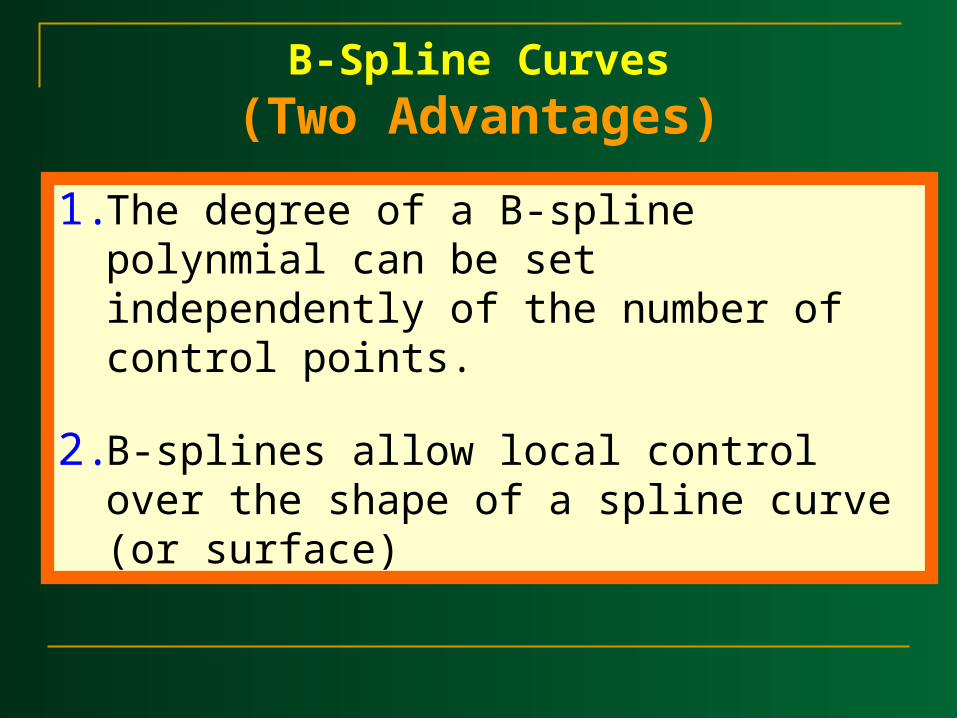
B-Spline Curves
(Two Advantages)
1. The degree of a B-spline polynmial can be set independently of the number of control points.
2. B-splines allow local control over the shape of a spline curve (or surface)

B-Spline Curves(Two Advantages)
A B-spline curve that is defined by 6 control point, and shows the effect of varying the degree of the polynomials (2,3, and 4)
Q3 is defined by P0,P1,P2,P3
Q4 is defined by P1,P2,P3,P4
Q5 is defined by P2,P3,P4,P5
Each curve segment shares
control points.

B-Spline Curves(Two Advantages)
The effect of changing the position of control
point P4 (locality property).

B-Spline Curves
Bézier Curve B-Spline Curve
B-Spline
Basis Functions

B-Spline Basis Functions(Knots, Knot Vector)
Let U be a set of m + 1 non-decreasing numbers, u0 <= u2 <= u3 <= ... <= um. The ui's are called knots,
The set U is the knot vectorknot vector.
muuuuU ,,,,
210
u1u0 u2 u3 u4 u5

B-Spline Basis Functions(Knots, Knot Vector)
The half-open interval [ui, ui+1) is the i-th knot span.
Some ui's may be equal, some knot spans may not exist.
m
uuuuU ,,,,210
B-Spline Basis Functions(Knots)
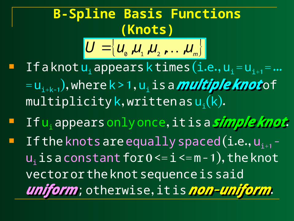
If a knot ui appears k times (i.e., ui = ui+1 = ... =
ui+k-1), where k > 1, ui is a multiple knotmultiple knot of multiplicity k, written as ui(k).
If ui appears only once, it is a simple knotsimple knot. If the knots are equally spaced (i.e., ui+1 - ui is a
constant for 0 <= i <= m - 1), the knot vector or the knot sequence is said uniformuniform; otherwise, it is non-uniformnon-uniform.
m
uuuuU ,,,,210

B-Spline Basis Functions
All B-spline basis functions are supposed to have their domain on [u0, um].
We use u0 = 0 and um = 1 frequently so that the domain is the closed interval [0,1].

B-Spline Basis Functions
To define B-spline basis functions, we need one more parameter.
The degree of these basis functions, p. The i-th B-spline basis function of degree p, written as Ni,p(u), is defined recursively as follows:
)()()(
otherwise0
if1)0(
1,111
11,,
10,
uNuu
uuuN
uu
uuuN
uuuN
piipi
pipi
ipi
ipi
iii
B-Spline Basis Functions
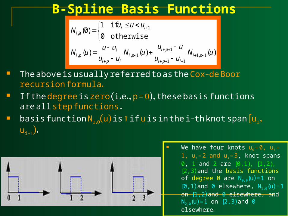
The above is usually referred to as the Cox-de Boor recursion formula.
If the degree is zero (i.e., p = 0), these basis functions are all step functions .
basis function Ni,0(u) is 1 if u is in the i-th knot span [ui, ui+1).
)()()(
otherwise0
if1)0(
1,111
11,,
10,
uNuu
uuuN
uu
uuuN
uuuN
piipi
pipi
ipi
ipi
iii
We have four knots u0 = 0, u1 = 1, u2 = 2 and u3 = 3, knot spans 0, 1 and 2 are [0,1), [1,2), [2,3) and the basis functions of degree 0 are N0,0(u) = 1 on [0,1) and 0 elsewhere, N1,0(u) = 1 on [1,2) and 0 elsewhere, and N2,0(u) = 1 on [2,3) and 0 elsewhere.

B-Spline Basis Functions To understand the way of computing Ni,p(u) for p
greater than 0, we use the triangular computation scheme.
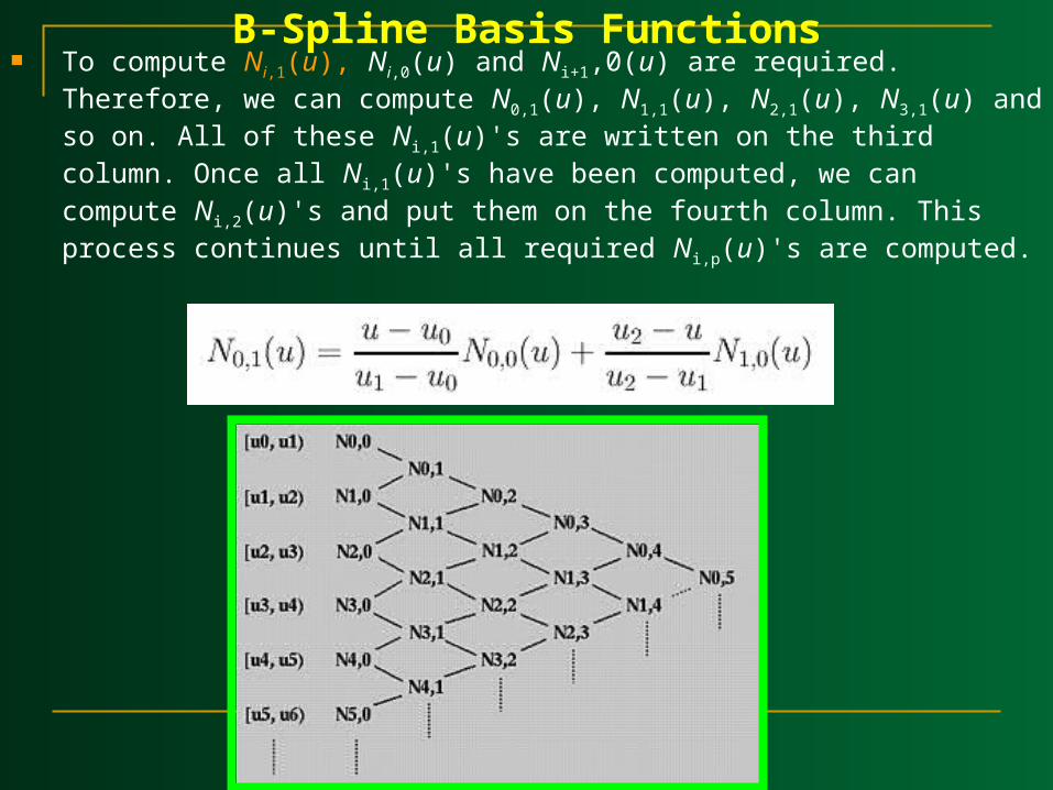
B-Spline Basis Functions To compute Ni,1(u), Ni,0(u) and Ni+1,0(u) are required. Therefore, we can
compute N0,1(u), N1,1(u), N2,1(u), N3,1(u) and so on. All of these Ni,1(u)'s are written on the third column. Once all Ni,1(u)'s have been computed, we can compute Ni,2(u)'s and put them on the fourth column. This process continues until all required Ni,p(u)'s are computed.
B-Spline Basis Functions
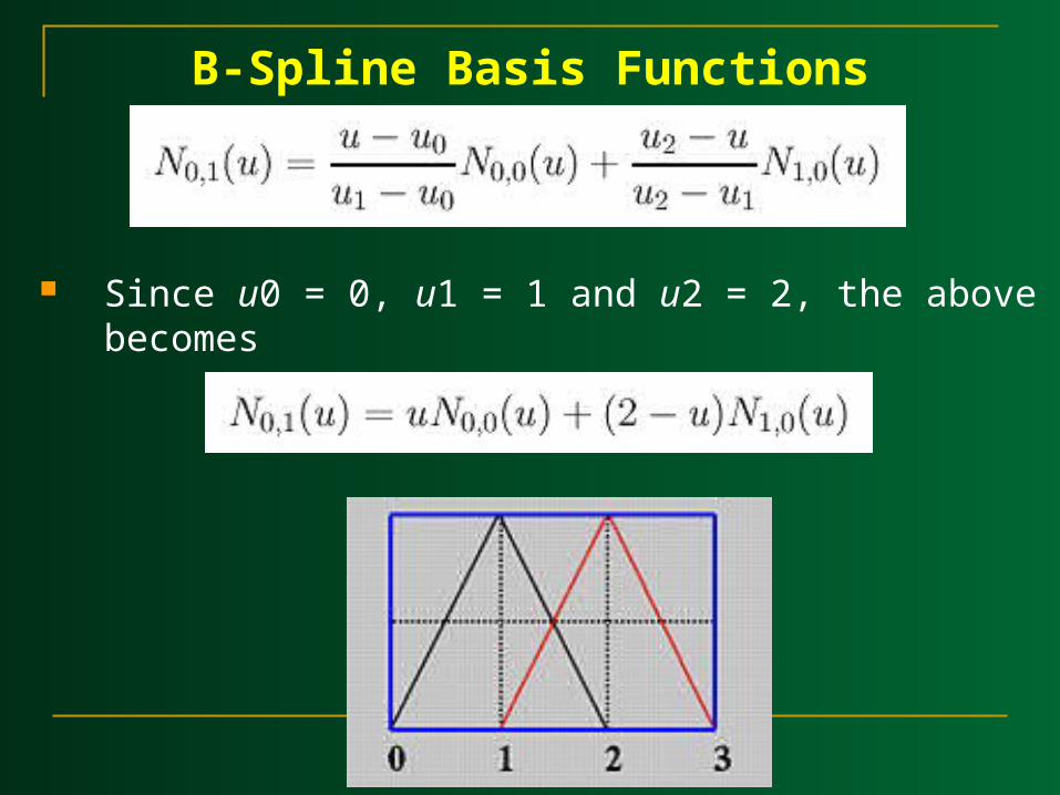
Since u0 = 0, u1 = 1 and u2 = 2, the above becomes
B-Spline Basis Functions
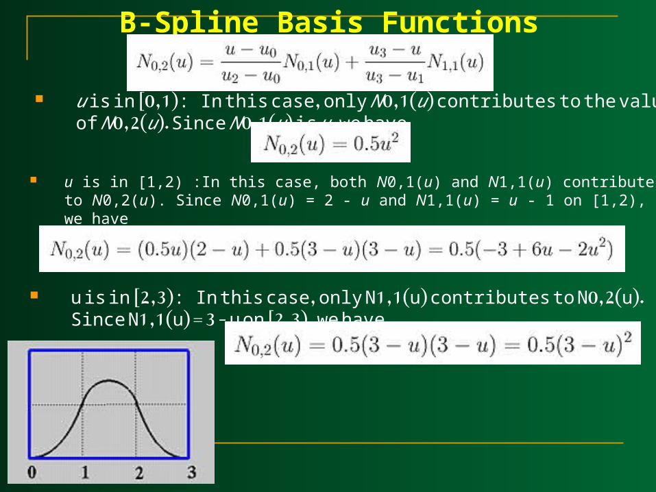
u is in [0,1): In this case, only N0,1(u) contributes to the value of N0,2(u). Since N0,1(u) is u, we have
u is in [1,2) :In this case, both N0,1(u) and N1,1(u) contribute to N0,2(u). Since N0,1(u) = 2 - u and N1,1(u) = u - 1 on [1,2), we have
u is in [2,3): In this case, only N1,1(u) contributes to N0,2(u). Since N1,1(u) = 3 - u on [2,3), we have

B-Spline Basis Functions

Two Important Observation
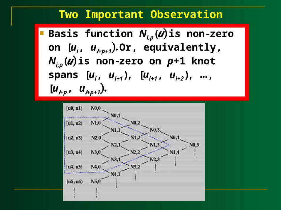
Basis function Ni,p(u) is non-zero on [ui, ui+p+1). Or, equivalently, Ni,p(u) is non-zero on p+1 knot spans [ui, ui+1), [ui+1, ui+2), ..., [ui+p, ui+p+1).
Two Important Observation
Two Important Observation
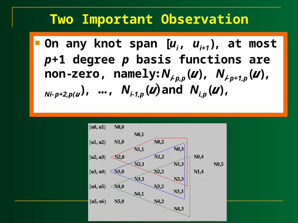
On any knot span [ui, ui+1), at most p+1 degree p basis functions are non-zero, namely: Ni-p,p(u), Ni-p+1,p(u), Ni-p+2,p(u), ..., Ni-
1,p(u) and Ni,p(u),

B-Spline Basis Functions(Important Properties )

B-Spline Basis Functions(Important Properties )
)()()(
otherwise0
if1)0(
1,111
11,,
10,
uNuu
uuuN
uu
uuuN
uuuN
piipi
pipi
ipi
ipi
iii
1. Ni,p(u) is a degree p polynomial in u.
2. Nonnegativity -- For all i, p and u, Ni,p(u) is non-negative
3. Local Support -- Ni,p(u) is a non-zero polynomial on [ui,ui+p+1)

B-Spline Basis Functions(Important Properties )
4. On any span [ui, ui+1), at most p+1 degree p basis functions are non-zero, namely: Ni-p,p(u), Ni-p+1,p(u), Ni-p+2,p(u), ..., and Ni,p(u) .
5. The sum of all non-zero degree p basis functions on span [ui, ui+1) is 1.
6. If the number of knots is m+1, the degree of the basis functions is p, and the number of degree p basis functions is n+1, then m = n + p + 1m = n + p + 1
B-Spline Basis Functions(Important Properties )
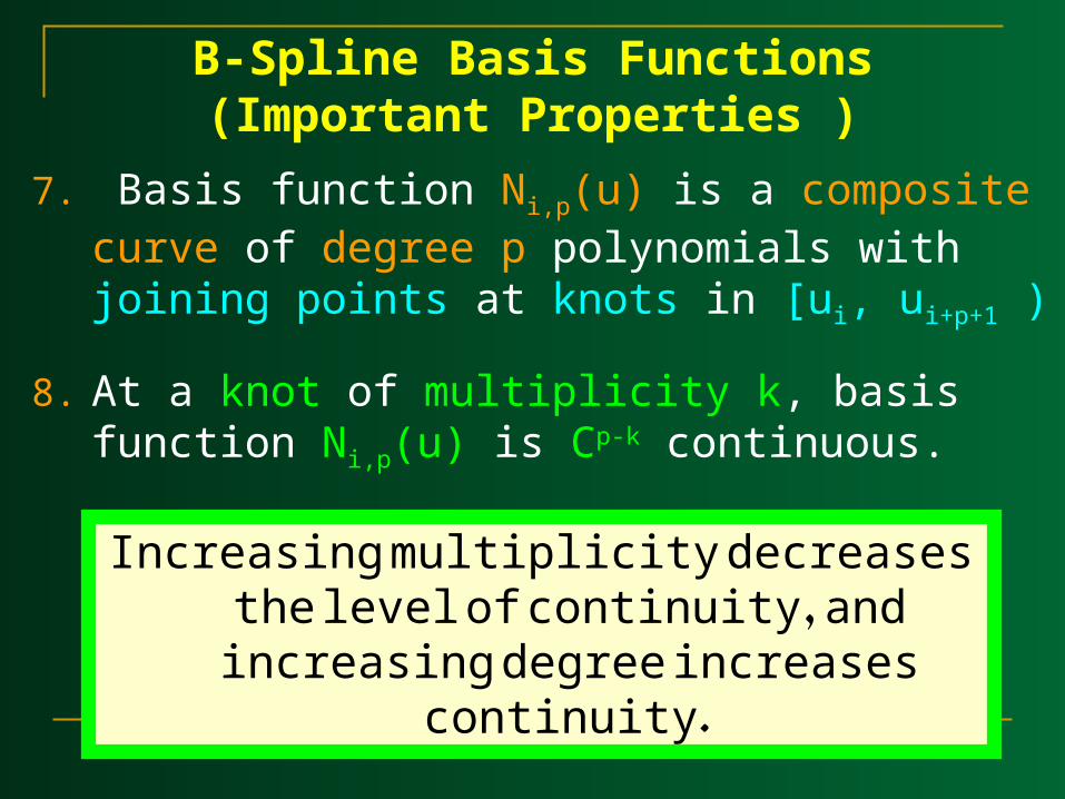
7. Basis function Ni,p(u) is a composite curve of degree p polynomials with joining points at knots in [ui, ui+p+1 )
8. At a knot of multiplicity k, basis function Ni,p(u) is Cp-k continuous.
Increasing multiplicity decreases the level of continuity, and increasing
degree increases continuity.

B-Spline Basis Functions(Computation Examples)
Simple Knots Suppose the knot vector is U = { 0, 0.25, 0.5, 0.75, 1 }.
Basis functions of degree 0: N0,0(u), N1,0(u), N2,0(u) and N3,0(u) defined on knot span [0,0.25,), [0.25,0.5), [0.5,0.75) and [0.75,1), respectively.

B-Spline Basis Functions(Computation Examples)
All Ni,1(u)'s (U = { 0, 0.25, 0.5, 0.75, 1 }(:
5.025.0)21(2
25.004)(
1,0 uu
uuuN
for
for
75.05.0for 3
5.025.0for 14)(1,1 uu
uuuN
175.0for )1(4
75.05.0for )12(2)(1,2 uu
uuuN
Since the internal knots 0.25, 0.5 and 0.75 are all simple (i.e., k = 1) and p = 1, there are p - k + 1 = 1 non-zero basis function and three
knots. Moreover, N0,1(u), N1,1(u) and N2,1(u) are C0 continuous at knots
0.25, 0.5 and 0.75, respectively.
B-Spline Basis Functions(Computation Examples)
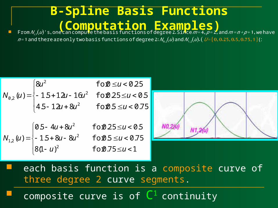
From Ni,1(u)'s, one can compute the basis functions of degree 2. Since m = 4, p = 2, and m = n + p + 1, we have n = 1 and
there are only two basis functions of degree 2: N0,2(u) and N1,2(u). (U = { 0, 0.25, 0.5, 0.75, 1 }(:
each basis function is a composite curve of three degree 2 curve segments.
composite curve is of C1 continuity
175.0for )1(8
75.05.0for 885.1
5.025.0for 845.0
)(2
2
2
2,1
uu
uuu
uuu
uN
75.05.0for 8125.4
5.025.0for 16125.1
25.00for 8
)(2
2
2
2,0
uuu
uuu
uu
uN

B-Spline Basis Functions (Computation Examples)
Knots with Positive Multiplicity :
Suppose the knot vector is U = { 0, 0, 0, 0.3, 0.5, 0.5, 0.6, 1, 1, 1{ Since m = 9 and p = 0 (degree 0 basis functions), we have n =
m - p - 1 = 8. there are only four non-zero basis functions of degree 0: N2,0(u), N3,0(u), N5,0(u) and N6,0(u).

B-Spline Basis Functions(Computation Examples)
Basis functions of degree 1: Since p is 1, n = m - p - 1 = 7. The following table shows the result
Basis Function Range Equation
N0,1(u) all u 0
N1,1(u) [0, 0.3) 1 - (10/3)u
N2,1(u)
[0, 0.3) (10/3)u
[0.3, 0.5) 2.5(1 - 2u)
N3,1(u) [0.3, 0.5) 5u - 1.5
N4,1(u) [0.5, 0.6) 6 - 10u
N5,1(u)
[0.5, 0.6) 10u - 5
[0.6, 1) 2.5(1 - u)
N6,1(u) [0.6, 1) 2.5u - 1.5
N7,1(u) all u 0
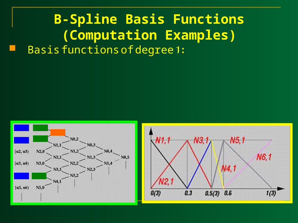
B-Spline Basis Functions(Computation Examples)
Basis functions of degree 1:

B-Spline Basis Functions(Computation Examples)
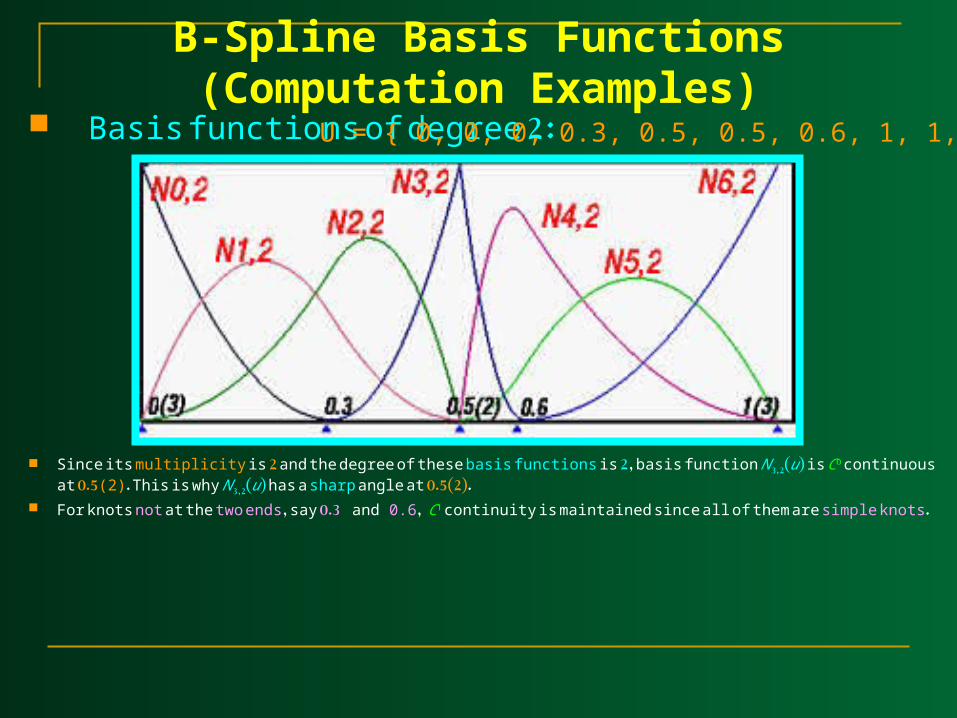
Since p = 2, we have n = m - p - 1 = 6. The following table contains all Ni,2(u)'s:
Function Range Equation
N0,2(u) [0, 0.3) (1 - (10/3)u)2
N1,2(u) [0, 0.3) (20/3)(u - (8/3)u2)
[0.3, 0.5) 2.5(1 - 2u)2
N2,2(u) [0, 0.3) (20/3)u2
[0.3, 0.5) -3.75 + 25u - 35u2
N3,2(u) [0.3, 0.5) (5u - 1.5)2
[0.5, 0.6) (6 - 10u)2
N4,2(u) [0.5, 0.6) 20(-2 + 7u - 6u2)
[0.6, 1) 5(1 - u)2
N5,2(u) [0.5, 0.6) 12.5(2u - 1)2
[0.6, 1) 2.5(-4 + 11.5u - 7.5u2)
N6,2(u) [0.6, 1) 2.5(9 - 30u + 25u2)
B-Spline Basis Functions(Computation Examples)
Basis functions of degree 2:
Since its multiplicity is 2 and the degree of these basis functions is 2, basis function N3,2(u) is C0 continuous at 0.5(2). This is why N3,2(u) has a sharp angle at 0.5(2).
For knots not at the two ends, say 0.3 and 0.6, C1 continuity is maintained since all of them are simple knots.
U = { 0, 0, 0, 0.3, 0.5, 0.5, 0.6, 1, 1, 1{

B-Spline
Curves

B-Spline Curves(Definition)
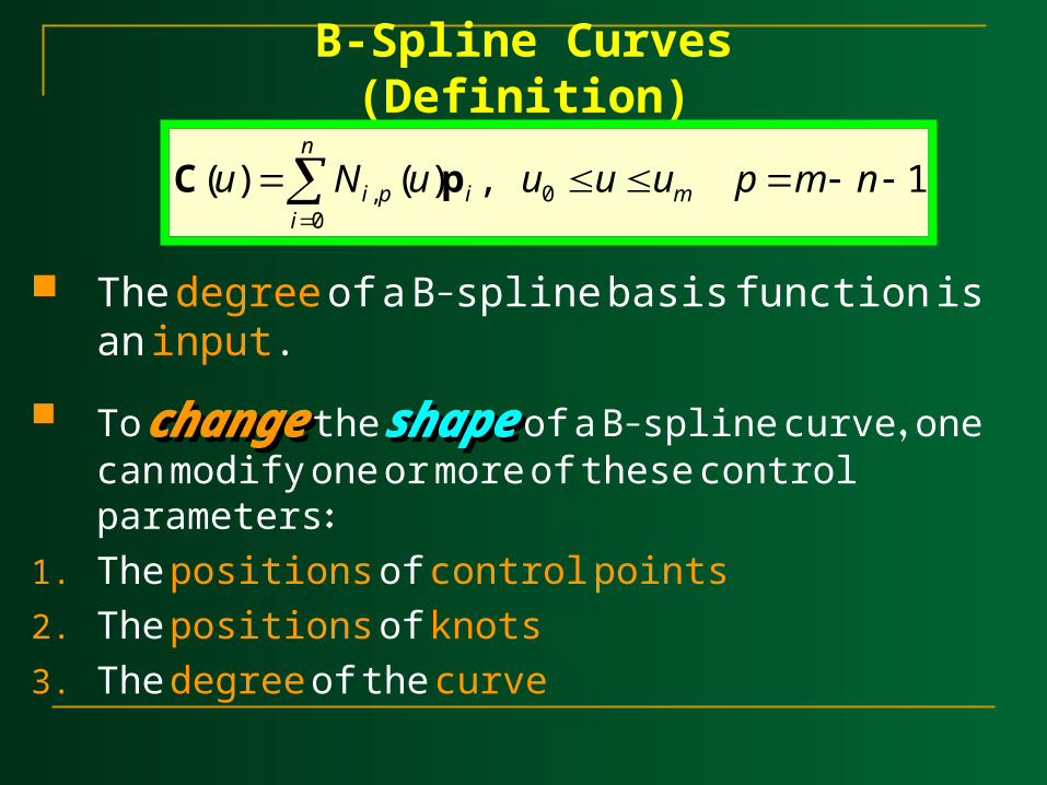
Given n + 1 control points P0, P1, ..., Pn and a knot vector U = { u0, u1, ..., um }, the B-
spline curve of degree p defined by these control points and knot vector U is
The point on the curve that corresponds to a knot ui, C(ui), is
referred to as a knot pointknot point. The knot points dividedivide a B-spline curve into curve segments,
each of which is defined on a knot span.
1,)()( 00
,
nmpuuuuNu m
n
iipi pC
B-Spline Curves(Definition)
The degree of a B-spline basis function is an input.
To changechange the shape shape of a B-spline curve, one can modify one or more of these control parameters:
1. The positions of control points
2. The positions of knots
3. The degree of the curve
1,)()( 00
,
nmpuuuuNu m
n
iipi pC
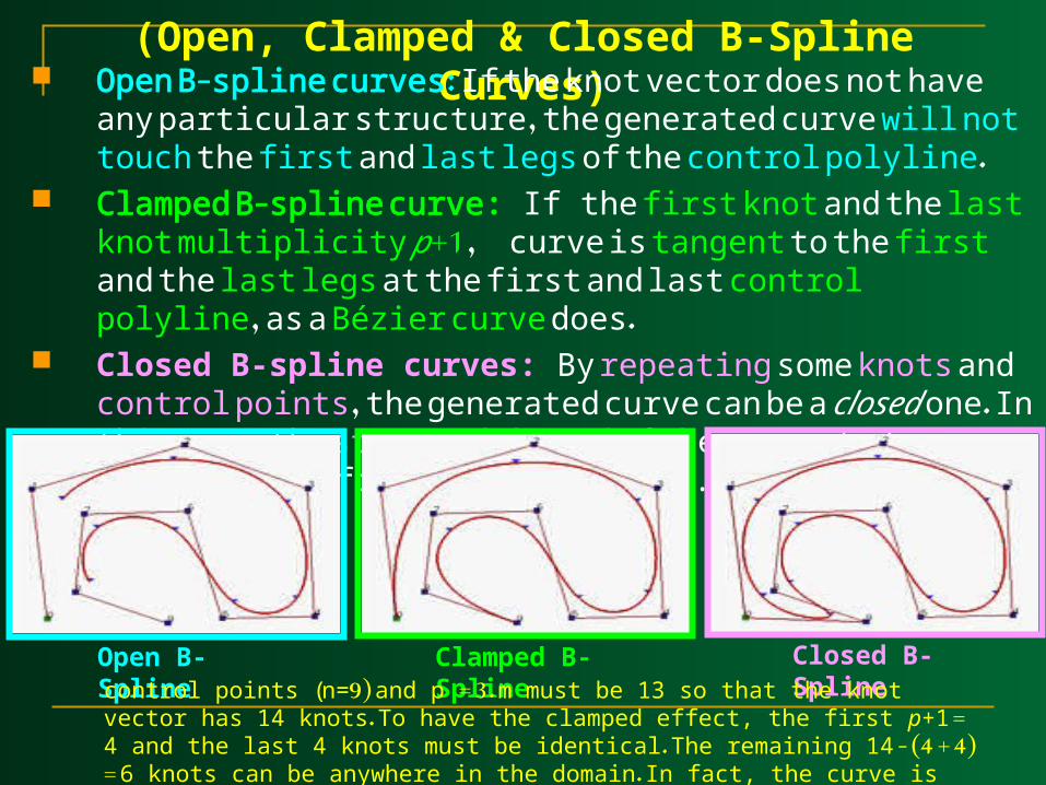
(Open, Clamped & Closed B-Spline Curves) Open B-spline curves: If the knot vector does not have any particular
structure, the generated curve will not touch the first and last legs of the control polyline.
Clamped B-spline curve: If the first knot and the last knot multiplicity p+1, curve is tangent to the first and the last legs at the first and last control polyline, as a Bézier curve does.
Closed B-spline curves: By repeating some knots and control points, the generated curve can be a closed one. In this case, the start and the end of the generated curve join together forming a closed loop.
Open B-Spline Clamped B-Spline Closed B-Splinecontrol points (n=9) and p = 3. m must be 13 so that the knot vector has 14 knots. To have the clamped effect, the first p+1 = 4 and the last 4 knots must be identical. The remaining 14 - (4 + 4) = 6 knots can be anywhere in the domain. In fact, the curve is generated with knot vector U = { 0, 0, 0, 0, 0.14, 0.28, 0.42, 0.57, 0.71, 0.85, 1, 1, 1, 1 }.

Open
B-Spline Curves

Open B-Spline Curves Recall from the B-spline basis function property that
on a knot span [ui, ui+1), there are at most p+1 non-zero basis functions of degree p.
For open B-spline curves, the domain is [up, um-p].
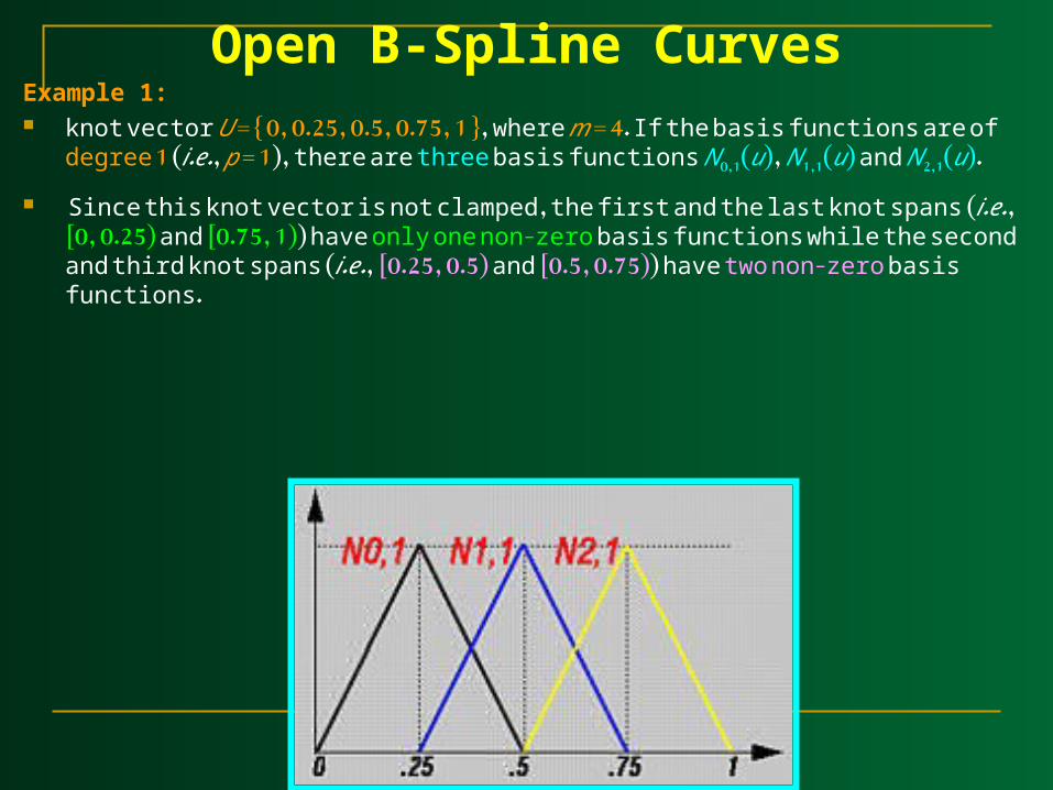
Open B-Spline CurvesExample 1: knot vector U = { 0, 0.25, 0.5, 0.75, 1 }, where m = 4. If the basis functions are of
degree 1 (i.e., p = 1), there are three basis functions N0,1(u), N1,1(u) and N2,1(u).
Since this knot vector is not clamped, the first and the last knot spans (i.e., [0, 0.25) and [0.75, 1)) have only one non-zero basis functions while the second and third knot spans (i.e., [0.25, 0.5) and [0.5, 0.75)) have two non-zero basis functions.

Open B-Spline CurvesExample 2:

Open B-Spline CurvesExample 3: A B-spline curve of degree 6 (i.e., p = 6) defined by 14 control points
(i.e., n = 13). The number of knots is 21 (i.e., m = n + p + 1 = 20). If the knot vector is uniform, the knot vector is }0, 0.05, 0.10, 0.15, ...,
0.90, 0.95,10{. The open curve is defined on [up, um-p] = [u6, u14] = [0.3, 0.7] and is not tangent to the first and last legs.
Clamped
B-Spline Curves

Clamped B-Spline Curves We use an exampleuse to illustrate the change between an open curve and a clamped one: An open B-spline curve of degree 4 , n = 8 and a uniform knot vector { 0, 1/13, 2/13, 3/13, ...,
12/13, 1 }. Multiplicity 5 (i.e., p+1),(second, third, fourth and fifth knot to 0 ) the curve not only passes
through the first control point but also is tangent to the first leg of the control polyline.

Closed
B-Spline Curves

Closed B-Spline Curves To construct a closed B-spline curve C(u) of degree p defined by n+1 control points ,the number of knots is m+1,
We mustWe must: 1. Design an uniform knot sequence of m+1 knots: u0 = 0, u1 = 1/m, u2 = 2/m, ..., um = 1. Note that the domain of the curve is
[up, un-p].
2.2. WrapWrap the first p and last p control points. More precisely, let P0 = Pn-p+1, P1 = Pn-p+2, ..., Pp-2 = Pn-1 and Pp-1 = Pn.
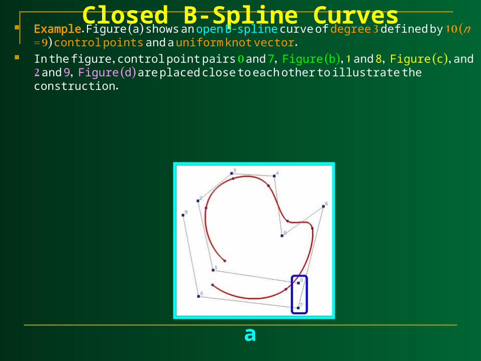
Closed B-Spline Curves Example. Figure (a) shows an open B-spline curve of degree 3 defined by 10
(n = 9) control points and a uniform knot vector. In the figure, control point pairs 0 and 7, Figure (b), 1 and 8, Figure (c), and 2
and 9, Figure (d) are placed close to each other to illustrate the construction.
a

Closed B-Spline Curves
a b
c d

B-Spline Curves
Important Properties

B-Spline Curves Important Properties1. B-spline curve C(u) is a piecewise curve with each component a curve of degree p. ٍ�Example: where n = 10, m = 14 and p = 3, the first four knots and last four knots are
clamped and the 7 internal knots are uniformly spaced. There are 8 knot spans, each of which corresponds to a curve segment.
Clamped B-Spline Curve Bézier Curve (degree 10!)

B-Spline Curves Important Properties2. Equality m = n + p + 1 must be satisfied.
3. Clamped B-spline curve C(u) passes through the two end control points P0 and Pn.
4. Strong Convex Hull Property: A B-spline curve is contained in the convex hull of its control polyline.

B-Spline Curves Important Properties
5. Local Modification Scheme: changing the position of control point Pi only affects the curve C(u) on interval [ui, ui+p+1).
The right figure shows the result of moving P2 to the lower right corner. Only the first, second and third curve segments change their shapes and all remaining curve segments stay in their original place without any change.

B-Spline Curves Important Properties A B-spline curve of degree 4 defined by 13 control points and 18 knots . Move P6.
The coefficient of P6 is N6,4(u), which is non-zero on [u6, u11). Thus, moving P6 affects curve segments 3, 4, 5, 6 and 7. Curve segments 1, 2, 8 and 9 are not affected.

B-Spline Curves Important Properties
6. C(u) is Cp-k continuous at a knot of multiplicity k
7. Affine Invariance


