74
Curved Surfaces & Tessellation Steve Rotenberg CSE168: Rendering Algorithms UCSD, Spring 2017
Curved Surfaces & Tessellation
Steve Rotenberg
CSE168: Rendering Algorithms
UCSD, Spring 2017
Curved Surfaces
• There are a variety of curved surface categories used in computer graphics:
– Parametric (explicit) surfaces
– Trimmed parametric surfaces
– Subdivision surfaces
– Implicit surfaces
Parametric Surface
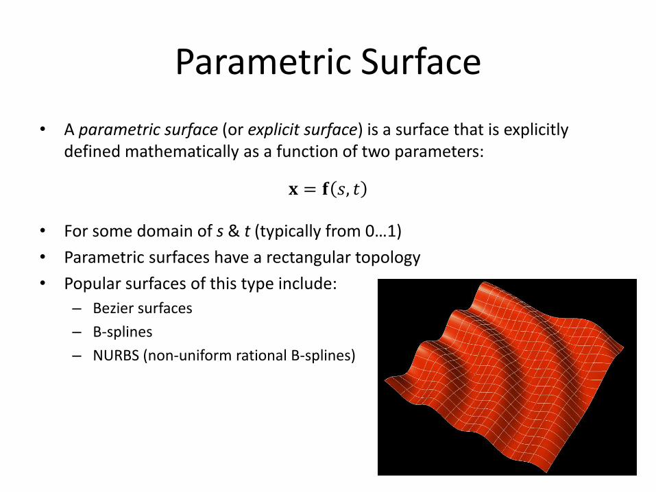
• A parametric surface (or explicit surface) is a surface that is explicitly defined mathematically as a function of two parameters:
𝐱 = 𝐟 𝑠, 𝑡
• For some domain of s & t (typically from 0…1)
• Parametric surfaces have a rectangular topology
• Popular surfaces of this type include:
– Bezier surfaces
– B-splines
– NURBS (non-uniform rational B-splines)
Trimmed Parametric Surfaces
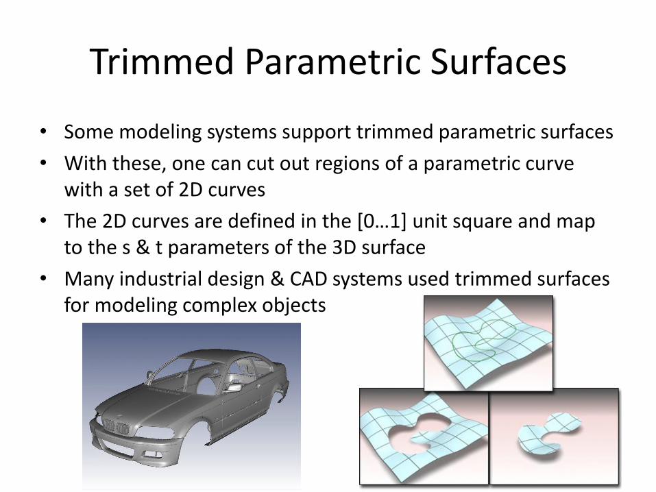
• Some modeling systems support trimmed parametric surfaces
• With these, one can cut out regions of a parametric curve with a set of 2D curves
• The 2D curves are defined in the [0…1] unit square and map to the s & t parameters of the 3D surface
• Many industrial design & CAD systems used trimmed surfaces for modeling complex objects
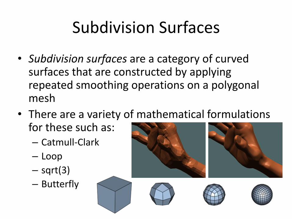
Subdivision Surfaces
• Subdivision surfaces are a category of curved surfaces that are constructed by applying repeated smoothing operations on a polygonal mesh
• There are a variety of mathematical formulations for these such as: – Catmull-Clark
– Loop
– sqrt(3)
– Butterfly
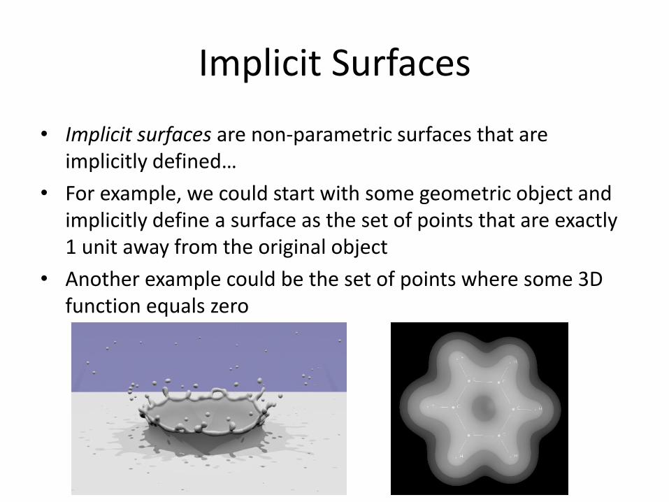
Implicit Surfaces
• Implicit surfaces are non-parametric surfaces that are implicitly defined…
• For example, we could start with some geometric object and implicitly define a surface as the set of points that are exactly 1 unit away from the original object
• Another example could be the set of points where some 3D function equals zero
Bezier Curves
Bezier
• Pierre Bézier (1910-1999) was a French engineer who made many early contributions to computational geometry and CAD modeling systems
• Much of his work was done while at Renault, where he worked for 42 years (1933-1975)
• He developed much of the mathematical theory and notation of Bezier curves, although the original algorithm was invented by Paul de Casteljau 1959, while working at Citroën
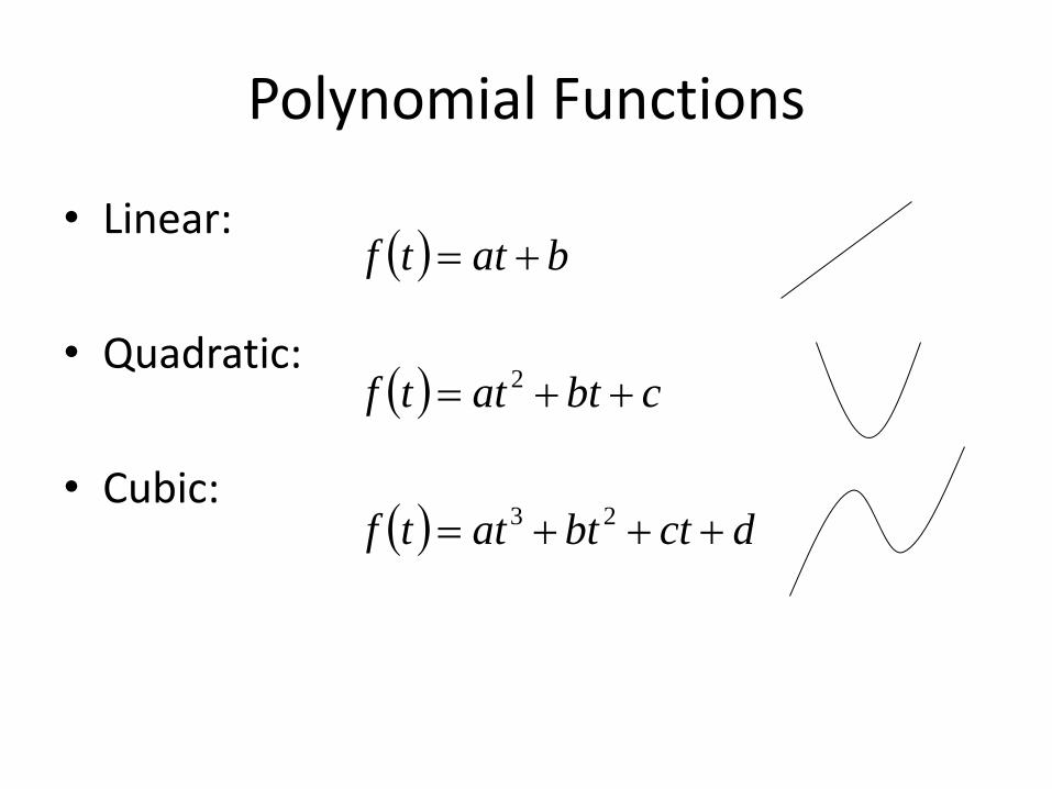
Polynomial Functions
• Linear:
• Quadratic:
• Cubic:
dctbtattf
cbtattf
battf
23
2
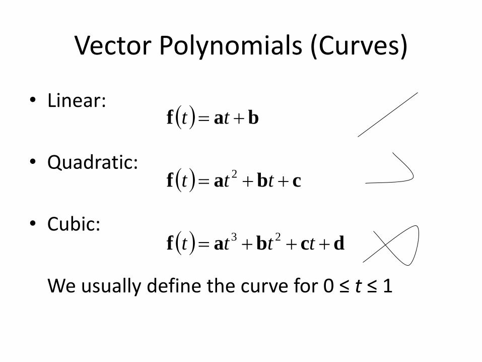
Vector Polynomials (Curves)
• Linear:
• Quadratic:
• Cubic:
We usually define the curve for 0 ≤ t ≤ 1
dcbaf
cbaf
baf
tttt
ttt
tt
23
2
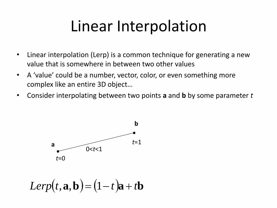
Linear Interpolation
• Linear interpolation (Lerp) is a common technique for generating a new value that is somewhere in between two other values
• A ‘value’ could be a number, vector, color, or even something more complex like an entire 3D object…
• Consider interpolating between two points a and b by some parameter t
baba tttLerp 1,,
a
b
t=1
. . 0<t<1
t=0
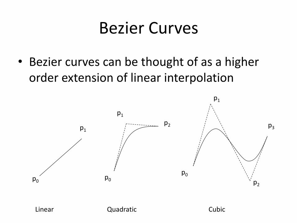
Bezier Curves
• Bezier curves can be thought of as a higher order extension of linear interpolation
p0
p1
p0
p1
p2
p0
p1
p2
p3
Linear Quadratic Cubic
de Casteljau Algorithm
• The de Casteljau algorithm describes the curve as a recursive series of linear interpolations
• This form is useful for providing an intuitive understanding of the geometry involved, and is very numerically stable, but it is not the most efficient form
de Casteljau Algorithm
p0
p1
p2
p3
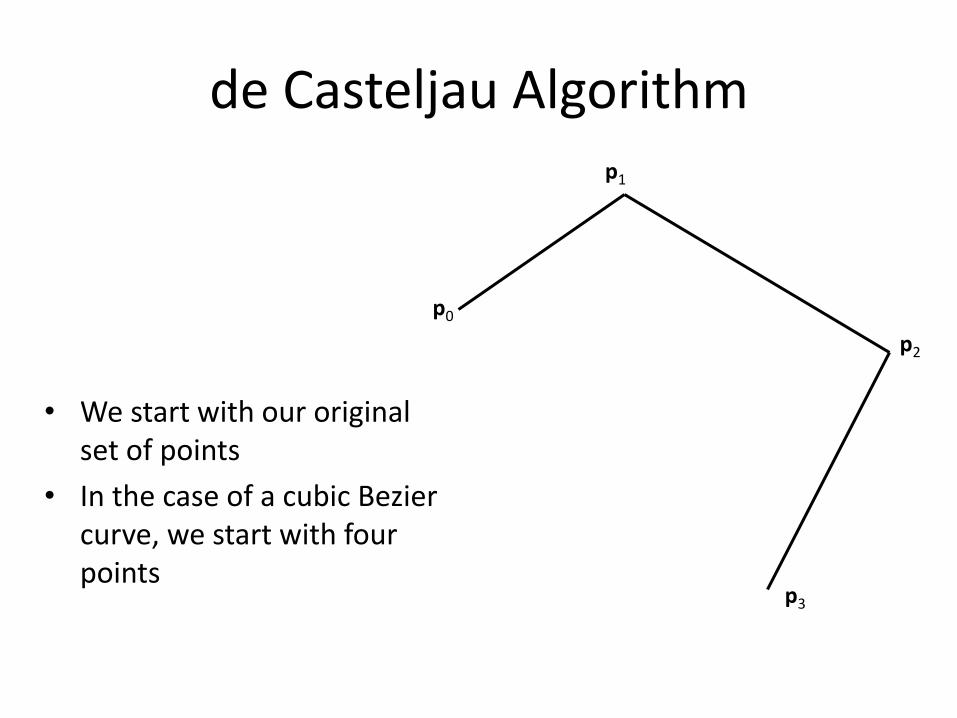
• We start with our original set of points
• In the case of a cubic Bezier curve, we start with four points
de Casteljau Algorithm
p0
p1
p2
p3
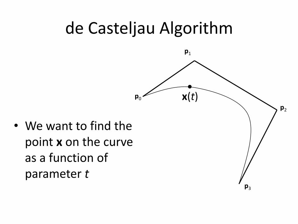
• We want to find the point x on the curve as a function of parameter t
x(t)
•
de Casteljau Algorithm
p0
q0
p1
p2
p3
q2
q1
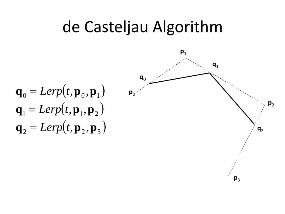
322
211
100
,,
,,
,,
ppq
ppq
ppq
tLerp
tLerp
tLerp
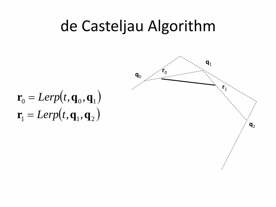
de Casteljau Algorithm
q0
q2
q1
r1
r0
211
100
,,
,,
qqr
qqr
tLerp
tLerp
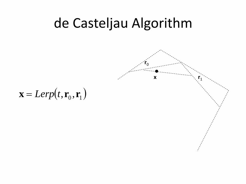
de Casteljau Algorithm
r1 x
r0
•
10 ,, rrx tLerp
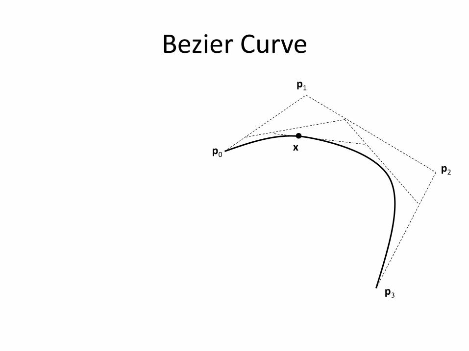
Bezier Curve
x
• p0
p1
p2
p3
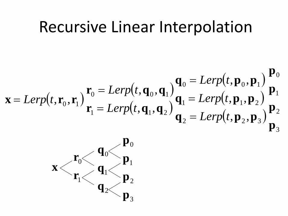
Recursive Linear Interpolation
322
211
100
,,
,,
,,
ppq
ppq
ppq
tLerp
tLerp
tLerp
211
100
,,
,,
qqr
qqr
tLerp
tLerp
10 ,, rrx tLerp
3
2
1
0
p
p
p
p
2
1
0
q
q
q
1
0
r
rx
3
2
1
0
p
p
p
p
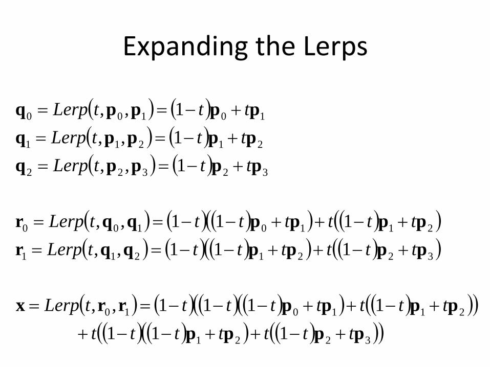
Expanding the Lerps
3221
211010
3221211
2110100
32322
21211
10100
111
1111,,
111,,
111,,
1,,
1,,
1,,
pppp
pppprrx
ppppqqr
ppppqqr
ppppq
ppppq
ppppq
ttttttt
ttttttttLerp
tttttttLerp
tttttttLerp
tttLerp
tttLerp
tttLerp
Cubic Equation Form
0
10
210
3210
23
010
2
210
3
3210
33
363
33
133
36333
pd
ppc
pppb
ppppa
dcbax
ppp
pppppppx
ttt
t
tt
3221
2110
111
1111
pppp
ppppx
ttttttt
ttttttt
Cubic Equation Form
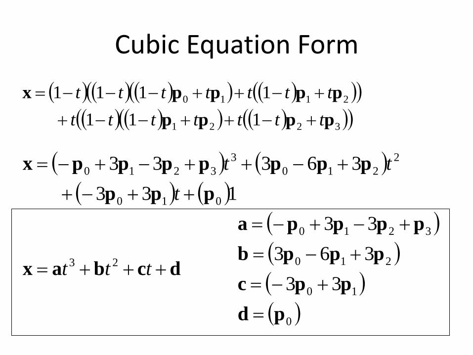
• If we regroup the equation by terms of exponents of t, we get it in the standard cubic form
• This form is very good for fast evaluation, as all of the constant terms (a,b,c,d) can be precomputed
• The cubic equation form obscures the input geometry (p0,p1,p2,p3), but there is a one-to-one mapping between the two and so the geometry can always be extracted out of the cubic coefficients

Matrix Form
0
10
210
3210
23
33
363
33
pd
ppc
pppb
ppppa
dcbax
ttt
3
2
1
0
23
0001
0033
0363
1331
1
p
p
p
p
d
c
b
a
d
c
b
a
x ttt
Matrix Form
zyx
zyx
zyx
zyx
ppp
ppp
ppp
ppp
ttt
ttt
333
222
111
000
23
3
2
1
0
23
0001
0033
0363
1331
1
0001
0033
0363
1331
1
x
p
p
p
p
x
Matrix Form
Ctx
GBtx
x
BezBez
zyx
zyx
zyx
zyx
ppp
ppp
ppp
ppp
ttt
333
222
111
000
23
0001
0033
0363
1331
1
Matrix Form
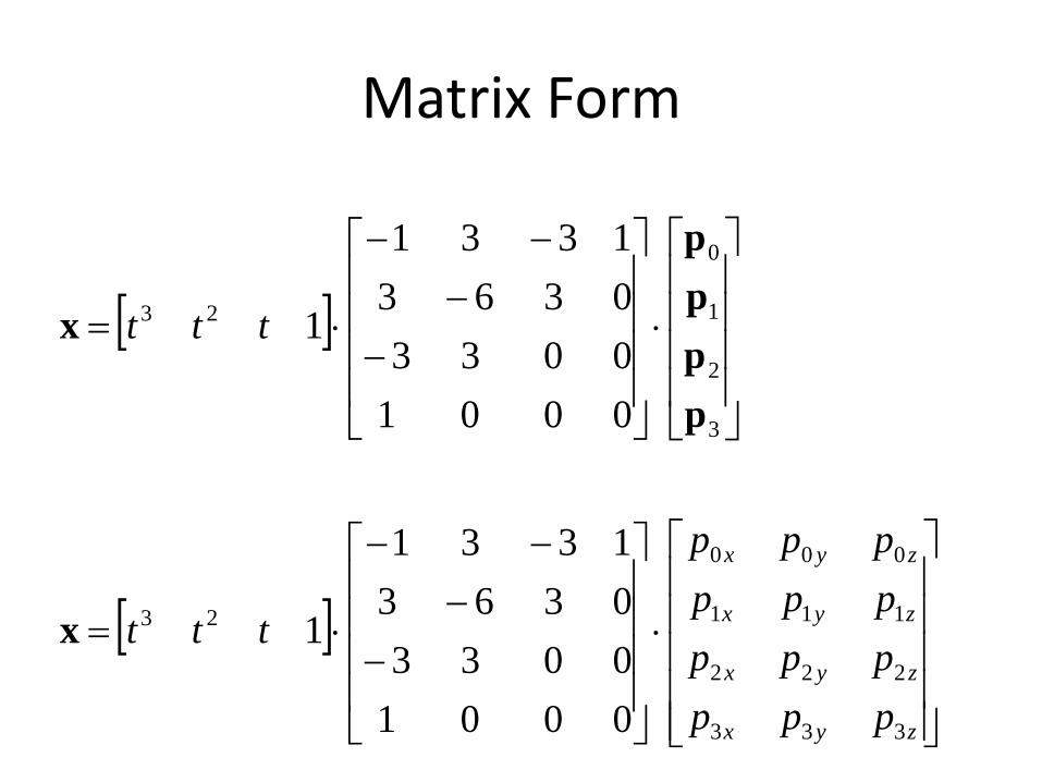
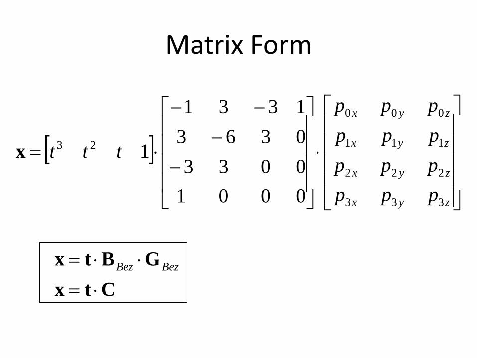
• We can rewrite the equations in matrix form
• This gives us a compact notation and shows how different forms of cubic curves can be related
• It also is a very efficient form as it can take advantage of existing 4x4 matrix hardware support…
Bezier Curves & Cubic Curves
• By adjusting the 4 control points of a cubic Bezier curve, we can represent any cubic curve
• Likewise, any cubic curve can be represented uniquely by a cubic Bezier curve
• There is a one-to-one mapping between the 4 Bezier control points (p0,p1,p2,p3) and the pure cubic coefficients (a,b,c,d)
• The Bezier basis matrix BBez (and it’s inverse) perform this mapping
• There are other common forms of cubic curves that also retain this property (Hermite, Catmull-Rom, B-Spline)
Tangents
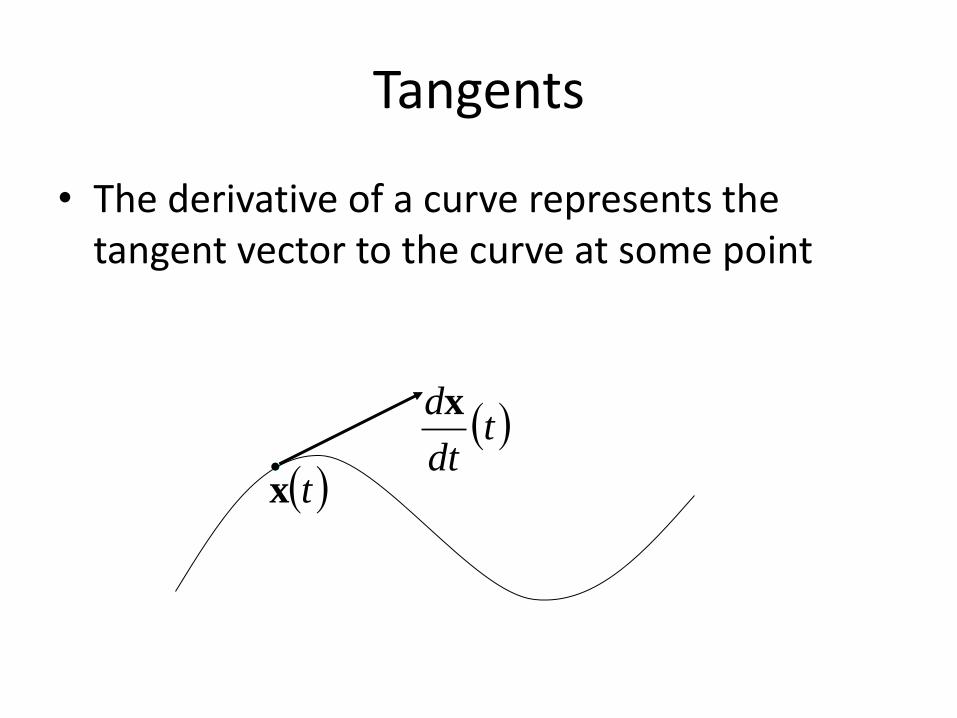
• The derivative of a curve represents the tangent vector to the curve at some point
tdt
dx
tx
Derivatives
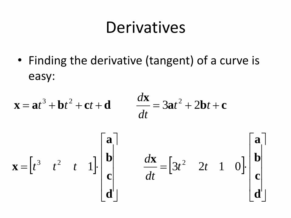
• Finding the derivative (tangent) of a curve is easy:
cbax
dcbax ttdt
dttt 23 223
d
c
b
a
x
d
c
b
a
x 01231 223 ttdt
dttt
Convex Hull Property
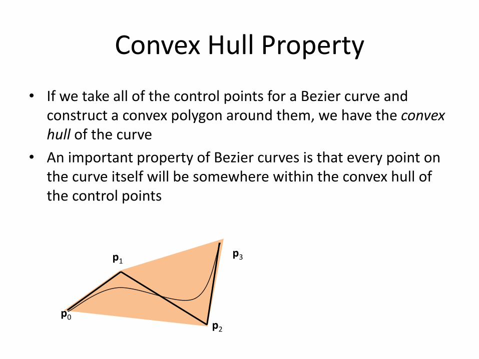
• If we take all of the control points for a Bezier curve and construct a convex polygon around them, we have the convex hull of the curve
• An important property of Bezier curves is that every point on the curve itself will be somewhere within the convex hull of the control points
p0
p1
p2
p3
Bezier Surfaces
Bezier Surfaces
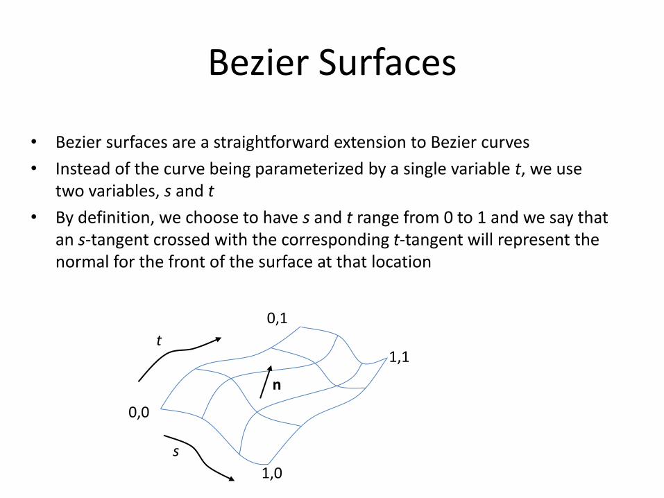
• Bezier surfaces are a straightforward extension to Bezier curves
• Instead of the curve being parameterized by a single variable t, we use two variables, s and t
• By definition, we choose to have s and t range from 0 to 1 and we say that an s-tangent crossed with the corresponding t-tangent will represent the normal for the front of the surface at that location
s
t
0,0
1,1
1,0
0,1
n
Control Mesh
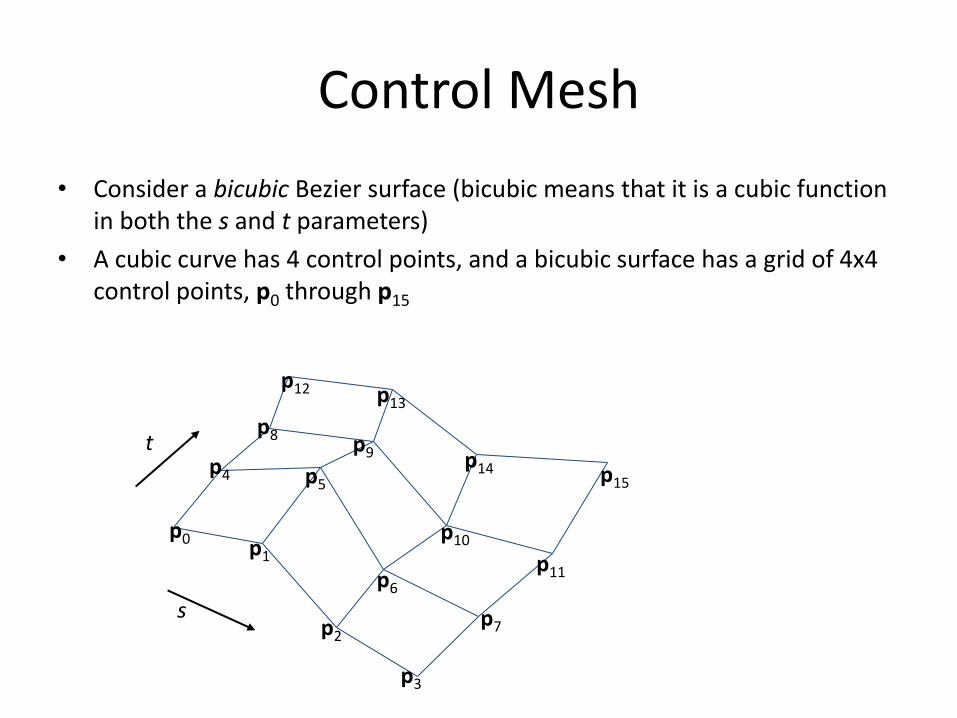
• Consider a bicubic Bezier surface (bicubic means that it is a cubic function in both the s and t parameters)
• A cubic curve has 4 control points, and a bicubic surface has a grid of 4x4 control points, p0 through p15
p0 p1
p2
p3
p4 p5
p6
p7
p8 p9
p10
p11
p12 p13
p14 p15
s
t
Surface Evaluation
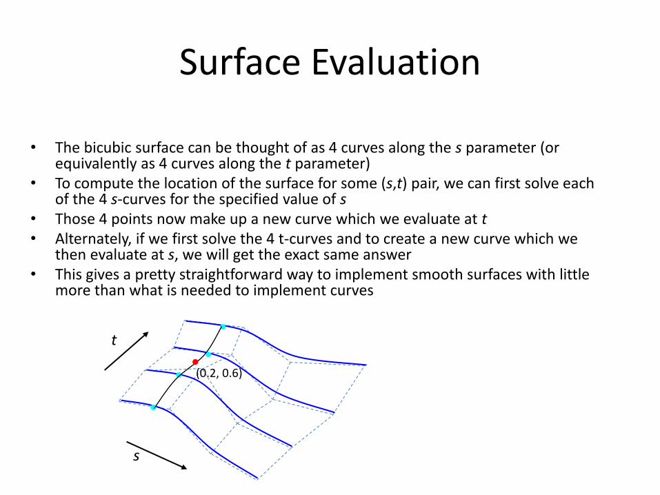
• The bicubic surface can be thought of as 4 curves along the s parameter (or equivalently as 4 curves along the t parameter)
• To compute the location of the surface for some (s,t) pair, we can first solve each of the 4 s-curves for the specified value of s
• Those 4 points now make up a new curve which we evaluate at t • Alternately, if we first solve the 4 t-curves and to create a new curve which we
then evaluate at s, we will get the exact same answer • This gives a pretty straightforward way to implement smooth surfaces with little
more than what is needed to implement curves
s
t
(0.2, 0.6)
Matrix Form
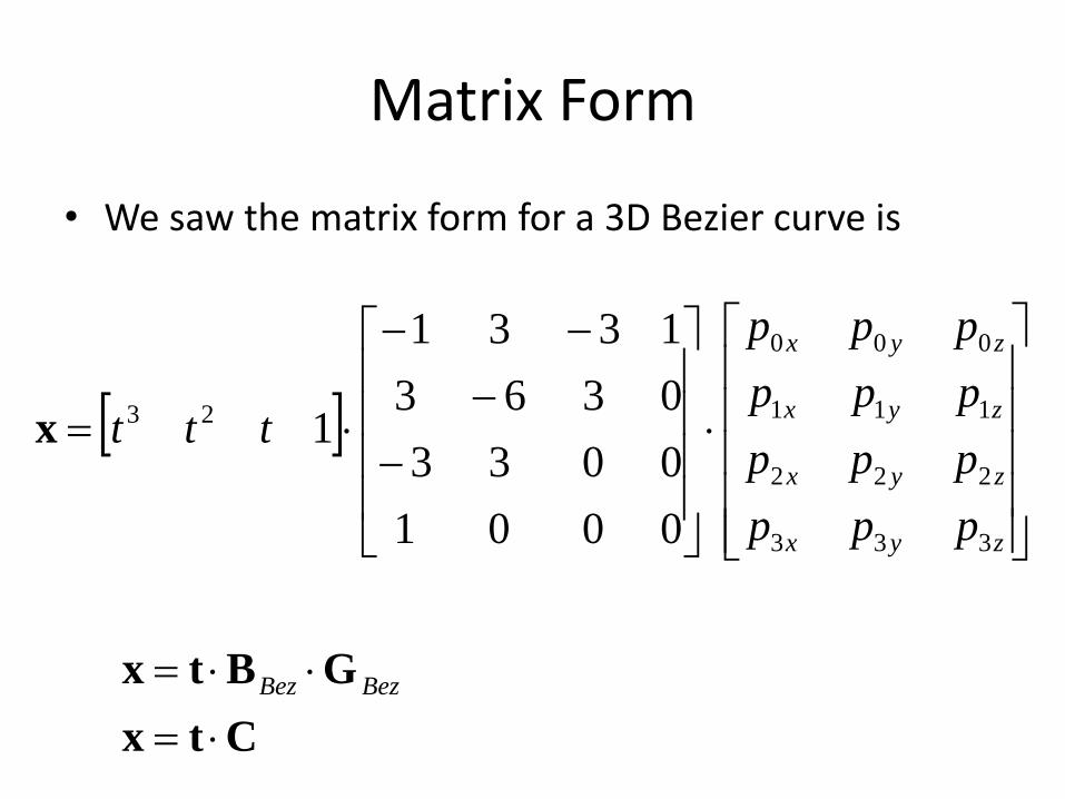
• We saw the matrix form for a 3D Bezier curve is
Ctx
GBtx
x
BezBez
zyx
zyx
zyx
zyx
ppp
ppp
ppp
ppp
ttt
333
222
111
000
23
0001
0033
0363
1331
1
Matrix Form
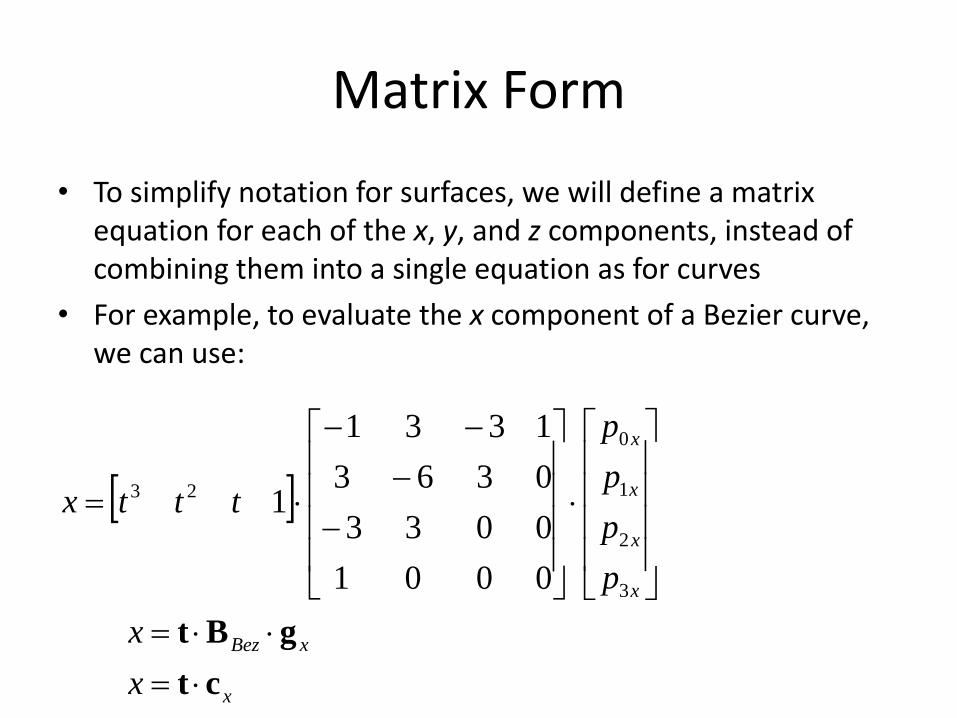
• To simplify notation for surfaces, we will define a matrix equation for each of the x, y, and z components, instead of combining them into a single equation as for curves
• For example, to evaluate the x component of a Bezier curve, we can use:
x
xBez
x
x
x
x
x
x
p
p
p
p
tttx
ct
gBt
3
2
1
0
23
0001
0033
0363
1331
1
Matrix Form
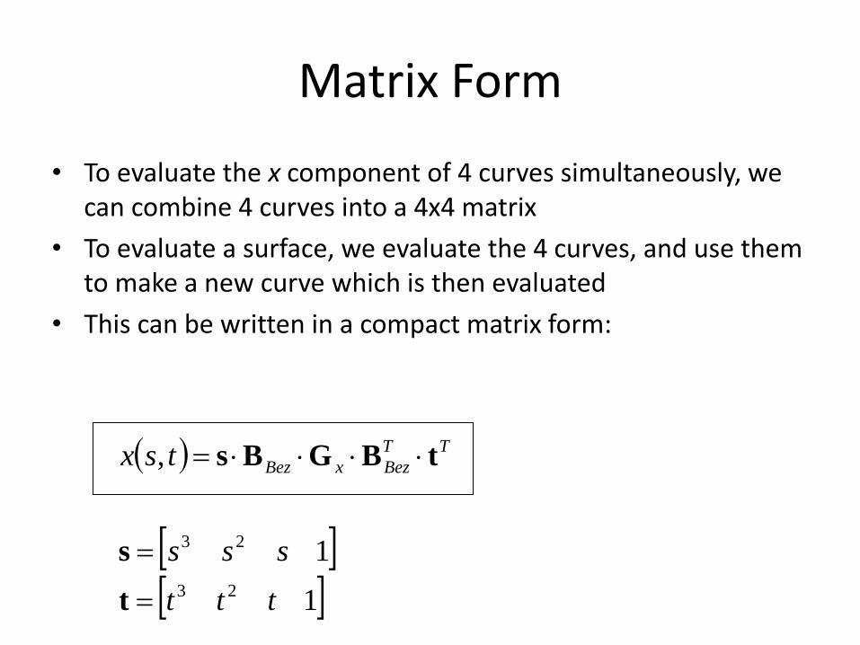
• To evaluate the x component of 4 curves simultaneously, we can combine 4 curves into a 4x4 matrix
• To evaluate a surface, we evaluate the 4 curves, and use them to make a new curve which is then evaluated
• This can be written in a compact matrix form:
1
1
,
23
23
ttt
sss
tsx TT
BezxBez
t
s
tBGBs
Matrix Form
1
1
,
23
23
ttt
sss
ts
T
BezxBezx
T
z
T
y
T
x
t
s
BGBC
tCs
tCs
tCs
x
xxxx
xxxx
xxxx
xxxx
x
T
BezBez
pppp
pppp
pppp
pppp
151173
141062
13951
12840
0001
0033
0363
1331
G
BB
Matrix Form
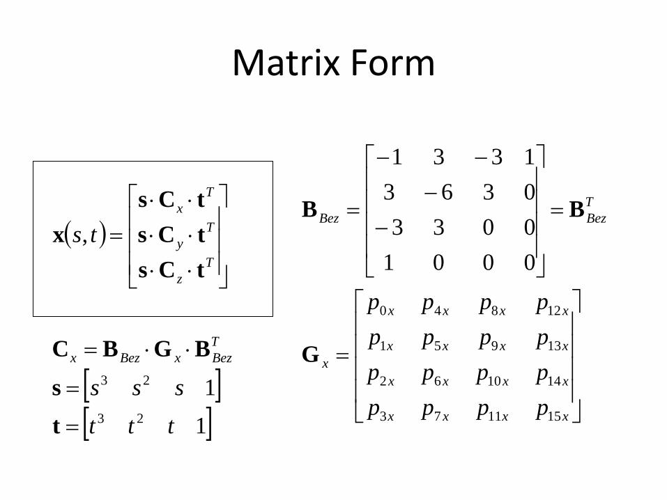
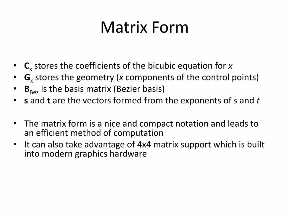
• Cx stores the coefficients of the bicubic equation for x • Gx stores the geometry (x components of the control points) • BBez is the basis matrix (Bezier basis) • s and t are the vectors formed from the exponents of s and t
• The matrix form is a nice and compact notation and leads to
an efficient method of computation • It can also take advantage of 4x4 matrix support which is built
into modern graphics hardware
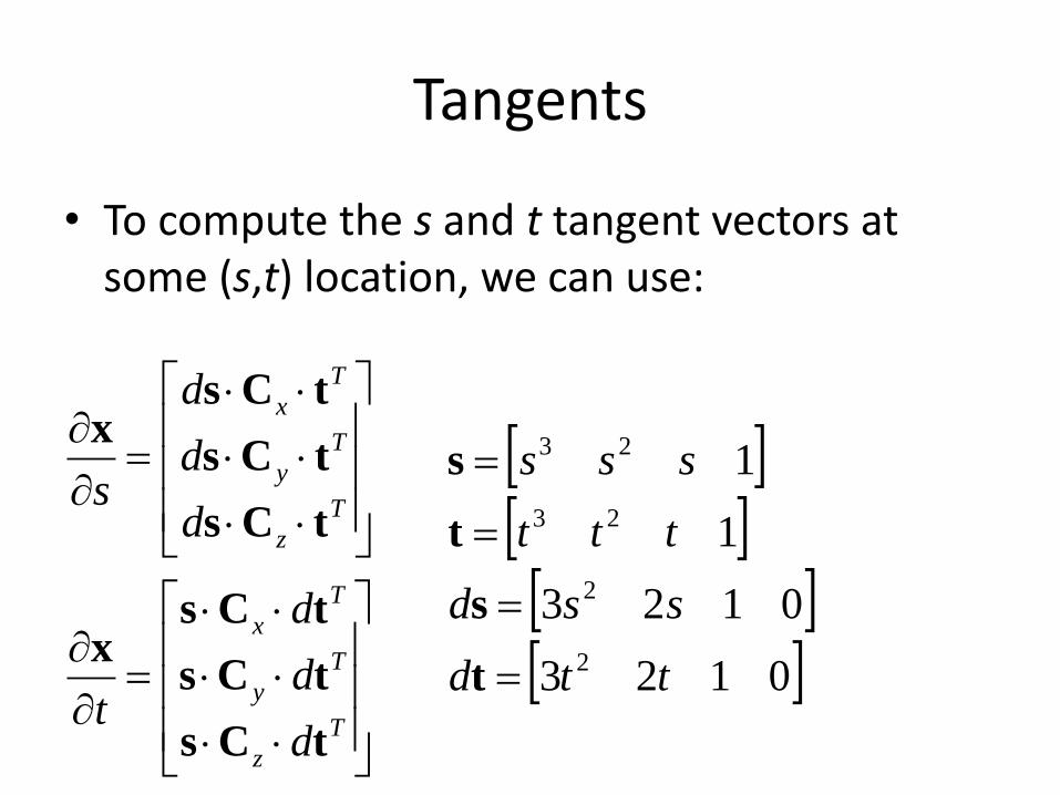
Tangents
• To compute the s and t tangent vectors at some (s,t) location, we can use:
T
z
T
y
T
x
T
z
T
y
T
x
d
d
d
t
d
d
d
s
tCs
tCs
tCsx
tCs
tCs
tCsx
0123
0123
1
1
2
2
23
23
ttd
ssd
ttt
sss
t
s
t
s
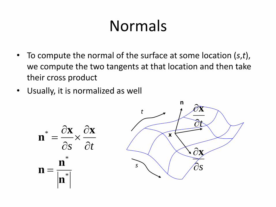
Normals
• To compute the normal of the surface at some location (s,t), we compute the two tangents at that location and then take their cross product
• Usually, it is normalized as well
*
*
*
n
nn
xxn
ts
s
t
n
x
s
x
t
x
Bezier Surface Properties
• Like Bezier curves, Bezier surfaces retain the convex hull property, so that any point on the actual surface will fall within the convex hull of the control points
• With Bezier curves, the curve will interpolate (pass through) the first and last control points, but will only approximate the other control points
• With Bezier surfaces, the 4 corners will interpolate, and the other 12 points in the control mesh are only approximated
• The 4 boundaries of the Bezier surface are just Bezier curves defined by the points on each edge of the surface
• By matching these points, two Bezier surfaces can be connected precisely
Tessellation
Tessellation
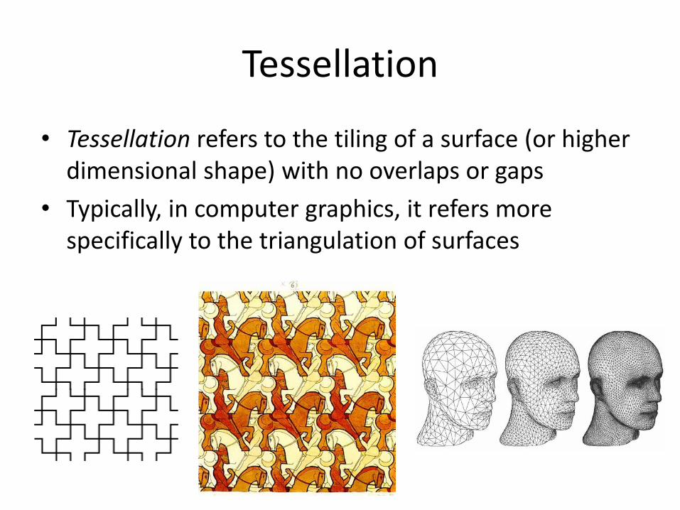
• Tessellation refers to the tiling of a surface (or higher dimensional shape) with no overlaps or gaps
• Typically, in computer graphics, it refers more specifically to the triangulation of surfaces
Tessellation
• For computer graphics purposes, tessellation is the process of triangulating a curved surface or other complex surface
• If we triangulate the surface before rendering, we can just insert those triangles into a spatial data structure and render as usual
• This is usually sufficient, as surfaces can be automatically tessellated to triangles that are the size of a single pixel or even smaller
Uniform Tessellation
• The most straightforward way to tessellate a parametric surface is uniform tessellation
• With this method, we simply choose some resolution in s and t and uniformly divide up the surface like a grid
• This method is very efficient to compute, as the cost of evaluating points on the surface is only slightly more costly than evaluating points on a curve
• However, as the generated mesh is uniform, it may have more triangles than it needs in flatter areas and fewer than it needs in highly curved areas
Adaptive Tessellation
• Very often, the goal of a tessellation is to provide the fewest triangles necessary to accurately represent the original surface
• For a curved surface, this means that we want more triangles in areas where the curvature is high, and fewer triangles in areas where the curvature is low
• We may also want more triangles in areas that are closer to the camera, and fewer farther away
• Adaptive tessellation schemes are designed to address these requirements
Recursive Tessellation
• Most adaptive tessellation approaches are recursive and use a top-down process
• We will first look at a recursive tessellation of a single curve, and then extend it to surfaces
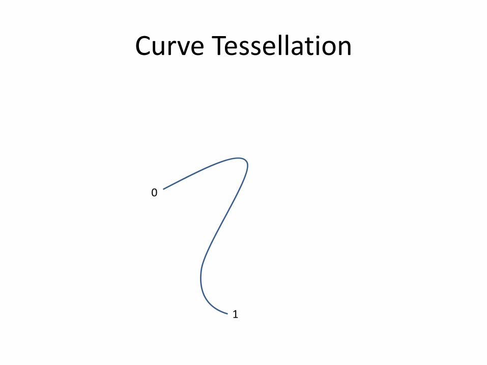
• We’ll assume that the curve is defined over the [0…1] domain in t • We start by examining the entire curve in that domain and consider
what would happen if we simply replaced it with a line segment • We then measure how well the line segment represents the
surface, and if we feel it is good enough, then we are done • Otherwise, the curve is subdivided into 2 curves and we repeat the
process recursively on each half
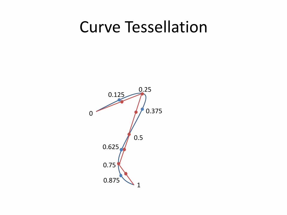
Recursive Tessellation
• How do we determine if a line segment is a good enough approximation to the curve?
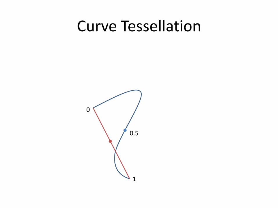
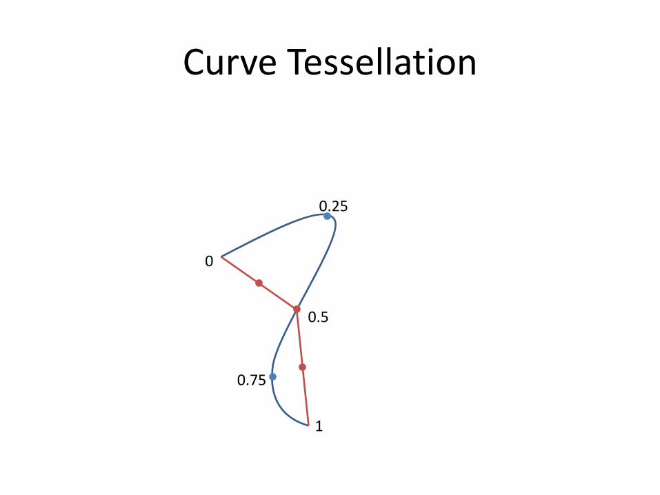
• There are many variations on this process, but a simple and common approach is to compare the midpoint of the line segment to the midpoint of the curve
• If they are within some specified distance, then we say it’s good enough
• Otherwise, we split
Curve Tessellation
0
1
Curve Tessellation
0
1
0.5
Curve Tessellation
0
1
0.5
0.25
0.75
Curve Tessellation
0
1
0.5
0.25
0.75
0.125
0.375
0.625
0.875
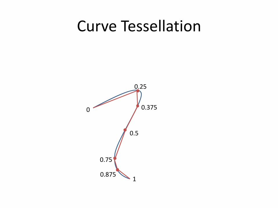
Curve Tessellation
0
1
0.5
0.25
0.75
0.375
0.875
Curve Tessellation Algorithm
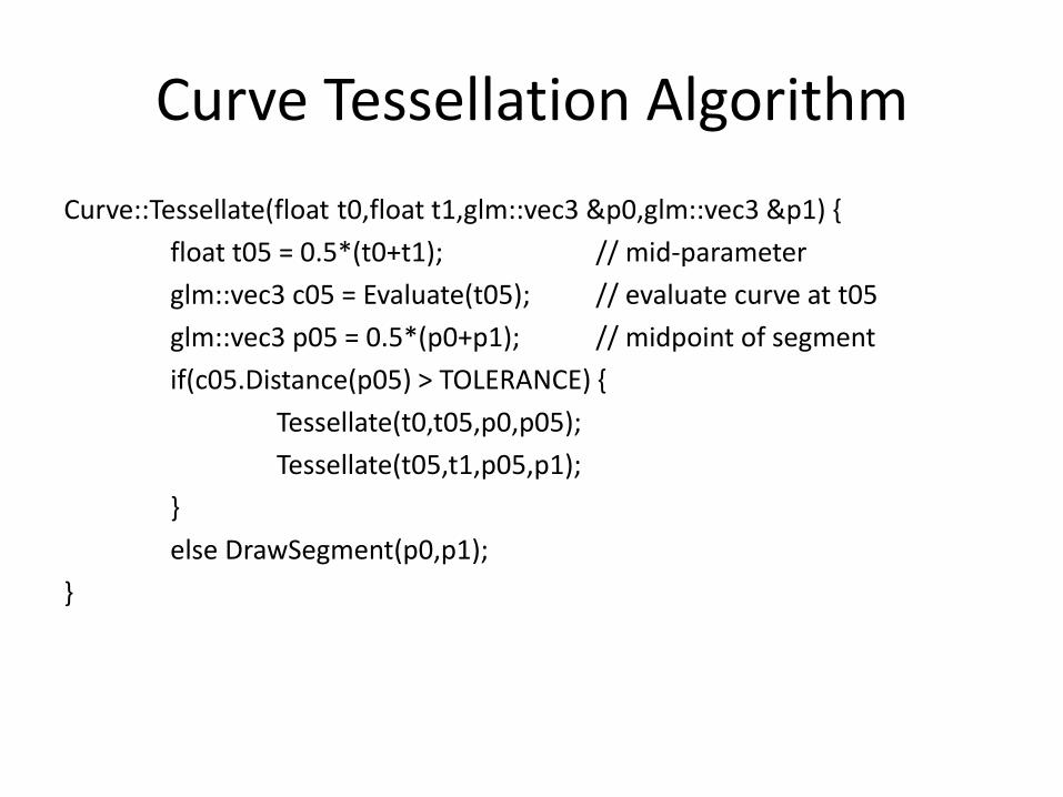
Curve::Tessellate(float t0,float t1,glm::vec3 &p0,glm::vec3 &p1) {
float t05 = 0.5*(t0+t1); // mid-parameter
glm::vec3 c05 = Evaluate(t05); // evaluate curve at t05
glm::vec3 p05 = 0.5*(p0+p1); // midpoint of segment
if(c05.Distance(p05) > TOLERANCE) {
Tessellate(t0,t05,p0,p05);
Tessellate(t05,t1,p05,p1);
}
else DrawSegment(p0,p1);
}

Subdivision Rules
• The previous example was based on comparing the distance of the midpoint of a curve to the midpoint of the approximating segment
• This process is generally pretty good and widely used, however there are a few potential problems and other issues
• For one thing, we could have a situation where the midpoint of the curve happens to hit the midpoint of the segment by chance, even though the two hardly match
• There are some practical ways to handle this
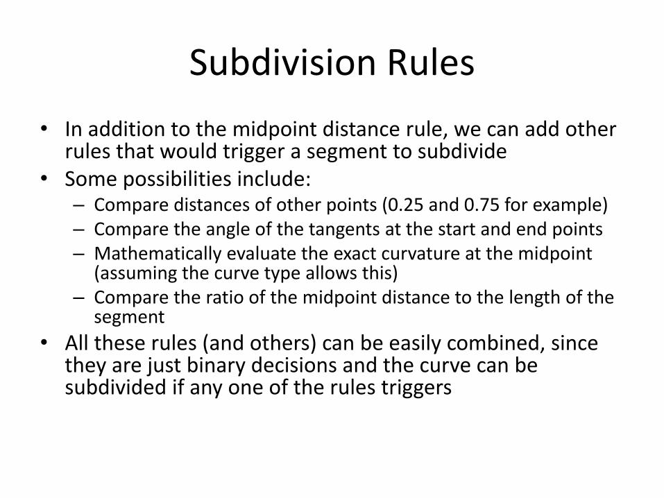
Subdivision Rules
• In addition to the midpoint distance rule, we can add other rules that would trigger a segment to subdivide
• Some possibilities include: – Compare distances of other points (0.25 and 0.75 for example) – Compare the angle of the tangents at the start and end points – Mathematically evaluate the exact curvature at the midpoint
(assuming the curve type allows this) – Compare the ratio of the midpoint distance to the length of the
segment
• All these rules (and others) can be easily combined, since they are just binary decisions and the curve can be subdivided if any one of the rules triggers
Pixel-Based Error
• One nice advantage of the midpoint distance approach is that it can be divided by the distance to the camera to provide a pixel based error measurement
• This provides a scheme for tessellating curves based on the error in pixels rather than the error in 3D distance
• This will cause curves closer to the camera to automatically adapt more than curves far away
Surface Tessellation
• Most adaptive tessellation approaches are recursive and use a top-down process
• We’ll assume that the surface is defined over the [0…1] domain in s and t
• We start by examining the entire surface in that domain and consider what would happen if we simply replaced it with two triangles
• We then measure how well the two triangles represent the surface, and if we feel it is good enough, then we are done
• Otherwise, the surface is subdivided (usually into 2 or 4 sub-surfaces) and we repeat the process recursively on each sub-surface
Surface Tessellation
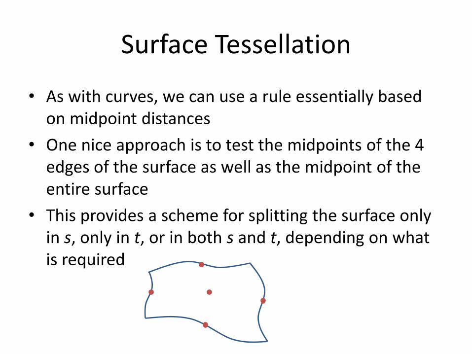
• As with curves, we can use a rule essentially based on midpoint distances
• One nice approach is to test the midpoints of the 4 edges of the surface as well as the midpoint of the entire surface
• This provides a scheme for splitting the surface only in s, only in t, or in both s and t, depending on what is required
`
Mixed Uniform/Adaptive Tessellation
• Some practical renderers use a mixed tessellation scheme • First, the original surface patch is adaptively subdivided into
several subpatches, each approximately the same size (say around 10 pixels on a side)
• Then, each of the subpatches (which is just a rectangular s,t range within the larger 0,1 rectangle) is uniformly tessellated to some resolution (say 10 x 10)
• The result is that the curved surface is tessellated into triangles roughly the size of a single pixel
• The bulk of the cost of the algorithm is in the uniform tessellation, which can be implemented in a very efficient way
Displacement Mapping
Displacement Mapping
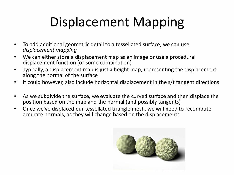
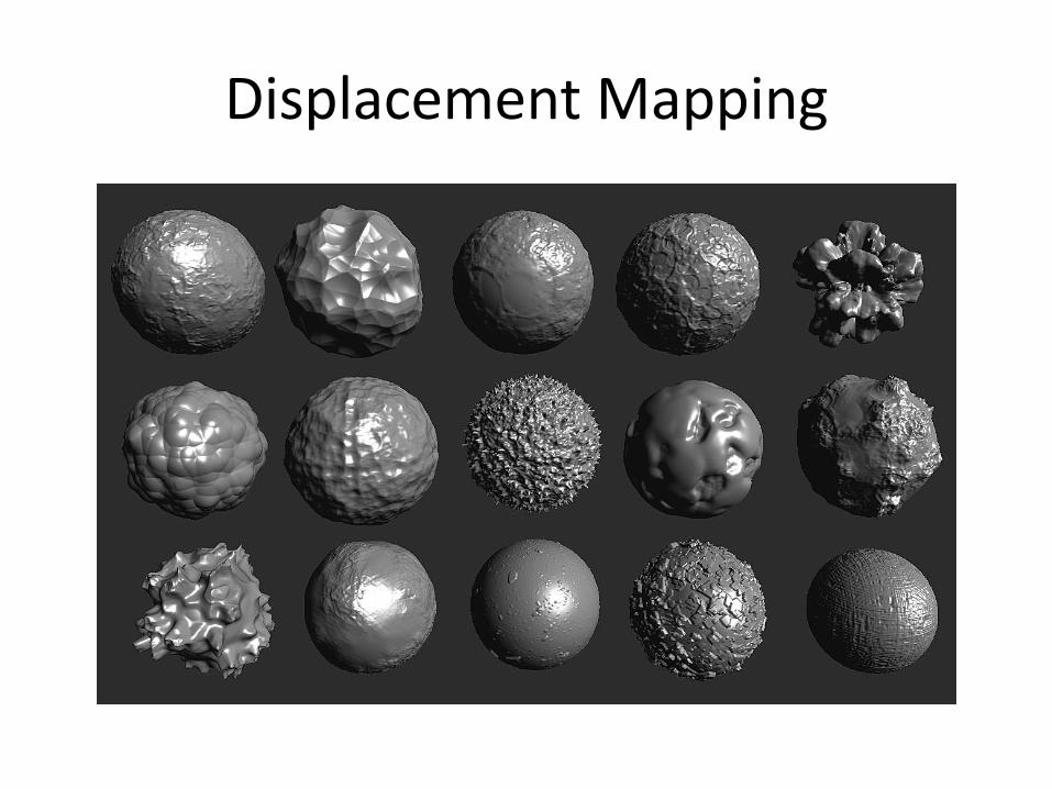
• To add additional geometric detail to a tessellated surface, we can use displacement mapping
• We can either store a displacement map as an image or use a procedural displacement function (or some combination)
• Typically, a displacement map is just a height map, representing the displacement along the normal of the surface
• It could however, also include horizontal displacement in the s/t tangent directions
• As we subdivide the surface, we evaluate the curved surface and then displace the position based on the map and the normal (and possibly tangents)
• Once we’ve displaced our tessellated triangle mesh, we will need to recompute accurate normals, as they will change based on the displacements
Displacement Mapping
Displacement Mapping
• The midpoint distance rule we discussed earlier is far less effective with displacement mapping
• The displacement map might have some localized area of high displacement that would be missed if we just looked at the midpoint
• Therefore, with displacement mapping, one typically has to subdivide the entire surface down to sub-pixel sized triangles to be certain to capture all the detail that might be in the map
• Alternately, one could do a lot of pre-processing on the map itself to identify areas of high displacement ahead of time, and drive the subdivision based on that (a min/max mipmap works well for this)
Ray Tracing Curved Surfaces
Ray Tracing Curved Surfaces
• There are several strategies for including curved surfaces into a ray tracer: – Pre-tessellation: before starting to render, we
tessellate the surface into a bunch of triangles and add them to a spatial data structure
– Lazy evaluation: tessellate and build a spatial data structure on the fly, as rays are tested against the surface
– Direct ray intersection: don’t tessellate at all. Every ray is intersected with the surface through a more direct means
Pre-Tessellation
• The pre-tessellation approach is the most common in practice due to its simplicity and high performance
• Curved surfaces can be pre-tessellated either based on 3D spatial properties and/or properties measured in pixel space
• One catch however, is with instanced objects
• We can’t really use pixel space metrics easily if we are using multiple copies of the geometry, each at different distances to the camera
Lazy Evaluation
• For the lazy evaluation approach, we start by only computing the bounding box of the entire surface
• When the bounding box is intersected by a ray, we then recursively subdivide the surface, computing bounding boxes of the sub-surfaces as we go
• We continue subdividing the boxes that the ray intersects until we generate triangles
• These are then kept in a box-tree-like data structure so they don’t need to be recomputed for the next ray that comes by
• This approach does essentially the same work as recursive subdivision combined with box-tree generation, but will have some performance overhead for the additional bookkeeping and complexity
• This approach might be useful if we didn’t expect rays to hit all of the surfaces, which might happen for simple renders, but wouldn’t be effective in a path tracer that bounces rays all over the place
• This approach can also be useful for extremely large scenes that don’t fit into memory. If combined with a system for deleting sections of the box-tree that haven’t been intersected for a while (or moving them to a slower, larger memory pool), we can create a system that fits within some fixed memory limit
Direct Intersection
• We can intersect rays directly with the surface if we want
• However, this is guaranteed to be much slower than pre-tessellated triangles, so it is only used in experimental cases or situations where memory is very limited
• Some surfaces can actually be mathematically intersected by solving the roots of a large polynomial
• Other surfaces are too complex and require a recursive subdivision, similar to the lazy evaluation, but without retention of the data structure for later use

Final Project
Final Project
• For the final project, you must add some features of your own choice to your renderer and render a final image
• Ideally, you could come up with a vision of what you want the final image to be and then implement the necessary features to achieve this, although you could also take the opposite approach and implement a bunch of features and then choose an idea that shows those off
• Also, it would be nice if it involved some different models than the standard test models
• This means you could search around online for some data and then write an appropriate importer, or even better- you could build something yourself in Blender, 3DStudio, or Maya and then import the data to your renderer
• The project should demonstrate at least one ‘complex’ feature and a few ‘simpler’ features (more details in the project description on the web page)
• You can also generate more than one image to show off different features, or you cold render an animation
• Provide an HTML page that shows the image and has a description of the features • Do a 5 minute live presentation during finals week
Final Project
• Some suggestions for ‘complex’ features: – Volumetric scattering – Procedural modeling – Displacement mapping – Dispersion – Caustics – Photon mapping – Translucency – Procedural texture – Curved surfaces, displacement mapping – Lens effects, convolution – Multi-frame animation with motion blur


