NOTICE: The author has granted a nonexclusive license allowing Library and Archives Canada to reproduce, publish, archive, preserve, conserve, communicate to the public by telecommunication or on the Internet, loan, distribute and sell theses worldwide, for commercial or noncommercial purposes, in microform, paper, electronic and/or any other formats.
AVIS: L'auteur a accorde une licence non exclusive permettant a la Bibliotheque et Archives Canada de reproduire, publier, archiver, sauvegarder, conserver, transmettre au public par telecommunication ou par Nntemet, preter, distribuer et vendre des theses partout dans le monde, a des fins commerciales ou autres, sur support microforme, papier, electronique et/ou autres formats.
The author retains copyright ownership and moral rights in this thesis. Neither the thesis nor substantial extracts from it may be printed or otherwise reproduced without the author's permission.
L'auteur conserve la propriete du droit d'auteur et des droits moraux qui protege cette these. Ni la these ni des extraits substantiels de celle-ci ne doivent etre imprimes ou autrement reproduits sans son autorisation.
In compliance with the Canadian Privacy Act some supporting forms may have been removed from this thesis.
While these forms may be included in the document page count, their removal does not represent any loss of content from the thesis.
Conformement a la loi canadienne sur la protection de la vie privee, quelques formulaires secondaires ont ete enleves de cette these.
Bien que ces formulaires aient inclus dans la pagination, il n'y aura aucun contenu manquant.
i*I
Canada Reproduced with permission of the copyright owner. Further reproduction prohibited without permission.
Abstract
As performance-based techniques become increasingly accepted in the design of
fire-safe buildings, the ability to predict the response of light-frame wood assemblies
exposed to realistic fire scenarios is needed. This work is part of a larger project at
Carleton University to develop a model to predict the risk from fire to occupants and
property in multi-storey non-residential buildings of light-frame wood construction.
A two-dimensional finite-element model called CUWoodFrame has been
developed to simulate the heat and mass transfer in both gypsum board and wood in
order to predict the thermal response of a wood-frame floor assembly exposed to fire.
The mass transfer analysis considers water vapour in gypsum board and both water
vapour and volatile pyrolysis products in wood. Calcination of gypsum board and
pyrolysis of wood are predicted using Arrhenius expressions. The evaporation of water
is modelled assuming the partial pressure of water vapour is equal to the equilibrium
vapour pressure.
Comparisons are made to tests conducted using the cone calorimeter, and
intermediate-scale and full-scale fire-resistance furnaces. Tests completed using the
cone entailed exposing a sample consisting of two layers of gypsum board protecting a
layer of wood to three different heat fluxes. The tests completed using the fire-
resistance furnaces were carried out using two different exposures. One test in each
furnace was conducted using the standard temperature-time curve, while the other was
subjected to an alternative exposure.
iii
Reproduced with permission of the copyright owner. Further reproduction prohibited without permission.
Comparisons between experiment and model predictions show good agreement
when comparing temperatures behind each layer of gypsum board. When modelling an
assembly, cavity temperatures are under-predicted resulting in an under-prediction of
the temperatures in the floor joist since the heat transfer to the joist is predominantly
from the cavity.
A sensitivity analysis has been conducted to study the variability in the
predictions of the model caused by uncertainties in the thermal and physical properties
of gypsum board and wood. Within the analysis, each parameter was varied based on
the variability reported in the literature. Results indicate the variability used in the
sensitivity analysis for thermal conductivity of gypsum board has the greatest impact on
the time until the wood begins to char.
IV
Reproduced with permission of the copyright owner. Further reproduction prohibited without permission.
Acknowledgements
I would like to express my appreciation to my thesis supervisors, Professor
George Hadjisophocleous and Professor Burkan Isgor. In particular, I would like to
thank Professor Hadjisophocleous for his optimistic support and commitment to both my
research and the Fire Safety Engineering Program at Carleton. I would like to thank
Professor Isgor for his many hours helping me through the development of the model and
modifying his own finite element program to meet the needs of this research. I would
especially like to thank Dr. Jim Mehaffey for his overwhelming support for this research
as well as my personal development as a research scientist.
I would also like to thank Mr. Les Richardson for his encouragement early on and
Richard Desjardins at FPInnovations - Forintek Division for his support and
understanding that allowed me to finish this thesis. I would like to thank Dr. Robert
White at the U.S. Forest Products Lab and John Latour at the National Research Council
for their assistance in carrying out the experiments. I would also like to acknowledge the
Natural Sciences and Engineering Research Council for the two post-graduate
scholarships I received; without this funding, this research would not have been possible.
Many thanks to my parents for their encouragement and guidance over the years.
Finally, I would like to thank my wife, Olivia, for her patience, endless encouragement
and loving support.
v
Reproduced with permission of the copyright owner. Further reproduction prohibited without permission.
Table of Contents
Abstract iii
Acknowledgements v
Table of Contents vi
List of Tables x
List of Figures xi
Nomenclature xviii
1. Introduction 1
1.1. Objective and Scope of Study 4
1.2. Contribution o f this Study 5
2. Literature Review 6
2.1. Standard Fire-Resistance Testing 6
2.1.1. Fire-resistance Floor Furnace and Test Assembly 7
2.1.2. Fire Exposure 8
2.1.3. Failure Criteria and Finish Rating 9
2.2. Previously Developed Thermal Models for Light-frame Construction 10
2.2.1. Thomas 10
2.2.2. Takeda and Mehaffey 11
2.2.3. Konig and Walleij 13
2.2.4. Clancy 14
2.2.5. Collier 15
2.2.6. Alfawakhiri 16
2.2.7. Hurst and Ahmed 16
2.2.8. Gammon 17
2.2.9. Manzello et al. 18
2.2.10. Fredlund 19
2.2.11. Sterner and Wickstrom 20
2.2.12. Summary of Available Models 21
2.3. Review of Material Properties 22
2.3.1. Gypsum Board 22
vi
Reproduced with permission of the copyright owner. Further reproduction prohibited without permission.
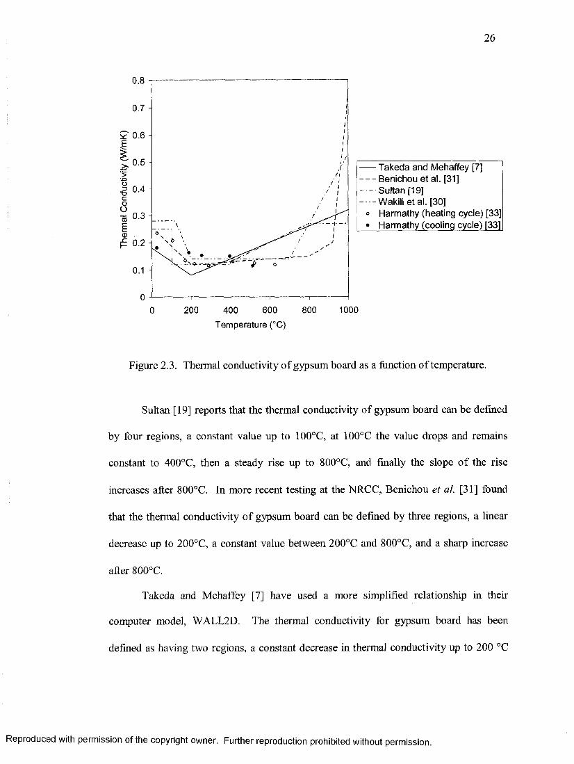
2.3.1.1. Gypsum Board Thermal Conductivity 25
2.3.1.2. Gypsum Board Apparent Specific Heat 28
2.3.1.3. Gypsum Board Density 30
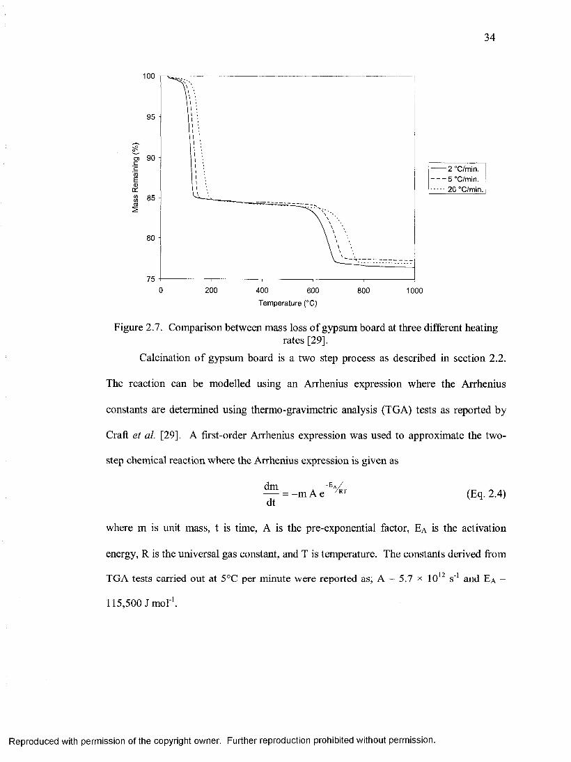
2.3.1.4. Calcination and Resulting Mass Loss of Gypsum 31
2.3.1.5. Gypsum Board Permeability 35
2.3.1.6. Gypsum Board Shrinkage 36
2.3.1.7. Gypsum Board Ablation 38
2.3.2. Wood 38
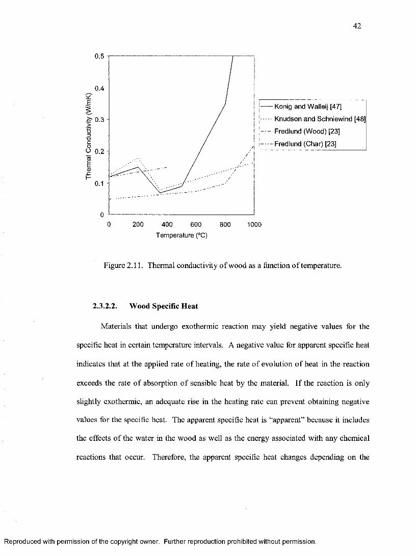
2.3.2.1. Wood Thermal Conductivity 40
2.3.2.2. Wood Specific Heat 42
2.3.2.3. Wood Density 45
2.3.2.4. Wood Porosity 45
2.3.2.5. Wood Permeability 46
2.3.2.6. Water in Wood 47
2.3.2.7. Volatile Pyrolysis Products 48
2.4. Review of Exposure Models and Measurements in Furnace 49
3. Model Description 53
3.1. Introduction 53
3.2. Heat Transfer Analysis 56
3.2.1. Governing Equations 56
3.2.1.1. Conduction T erms 61
3.2.1.2. Advection Terms 61
3.2.1.3. SourceTerms 64
3.2.1.4. Transient Term 64
3.3. Mass Transfer Analysis 66
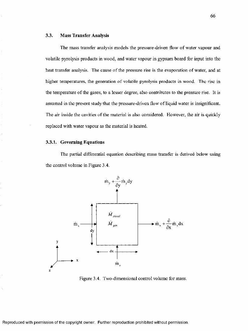
3.3.1. Governing Equations 66
3.3.2. Mass Flow Rates 73
3.4. Solution Methodology 73
4. Experimental Program 76
4.1. Cone Calorimeter Tests 76
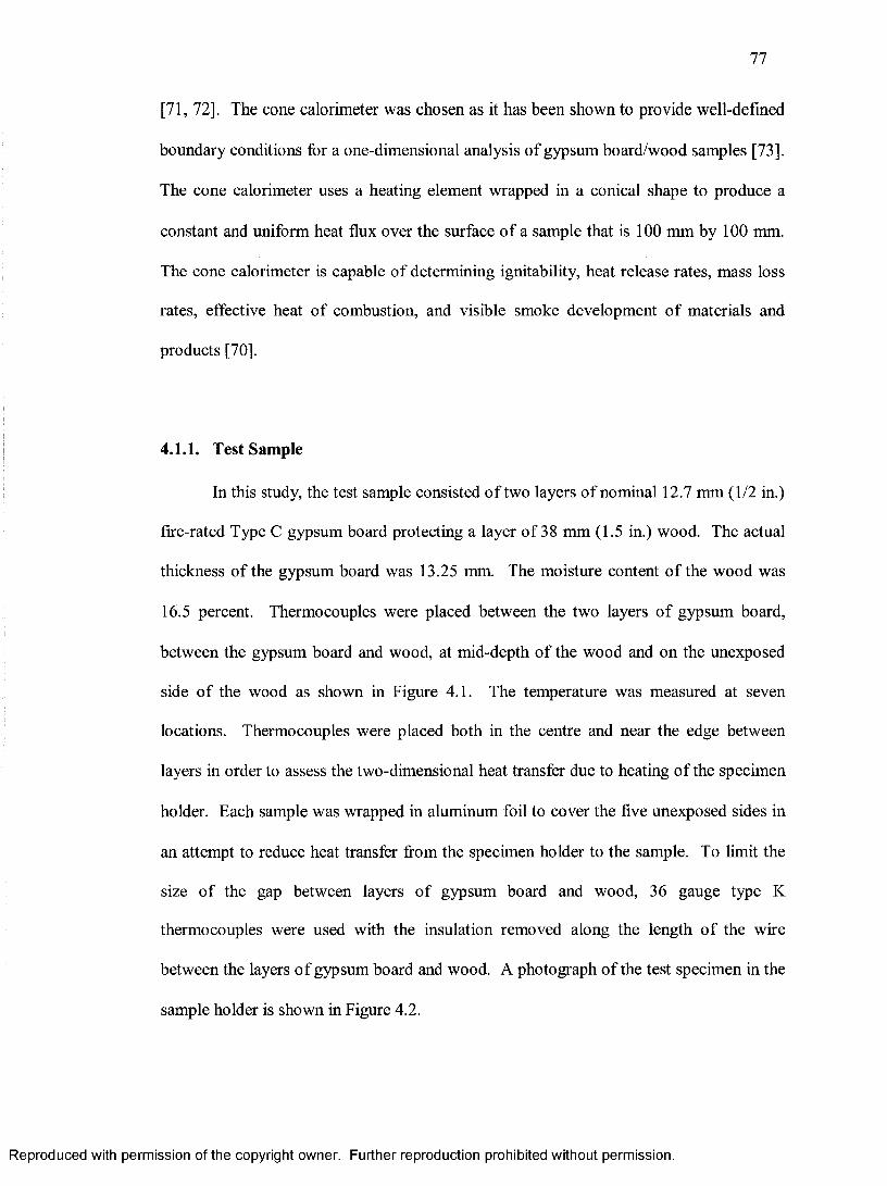
4.1.1. Test Sample 77
vii
Reproduced with permission of the copyright owner. Further reproduction prohibited without permission.
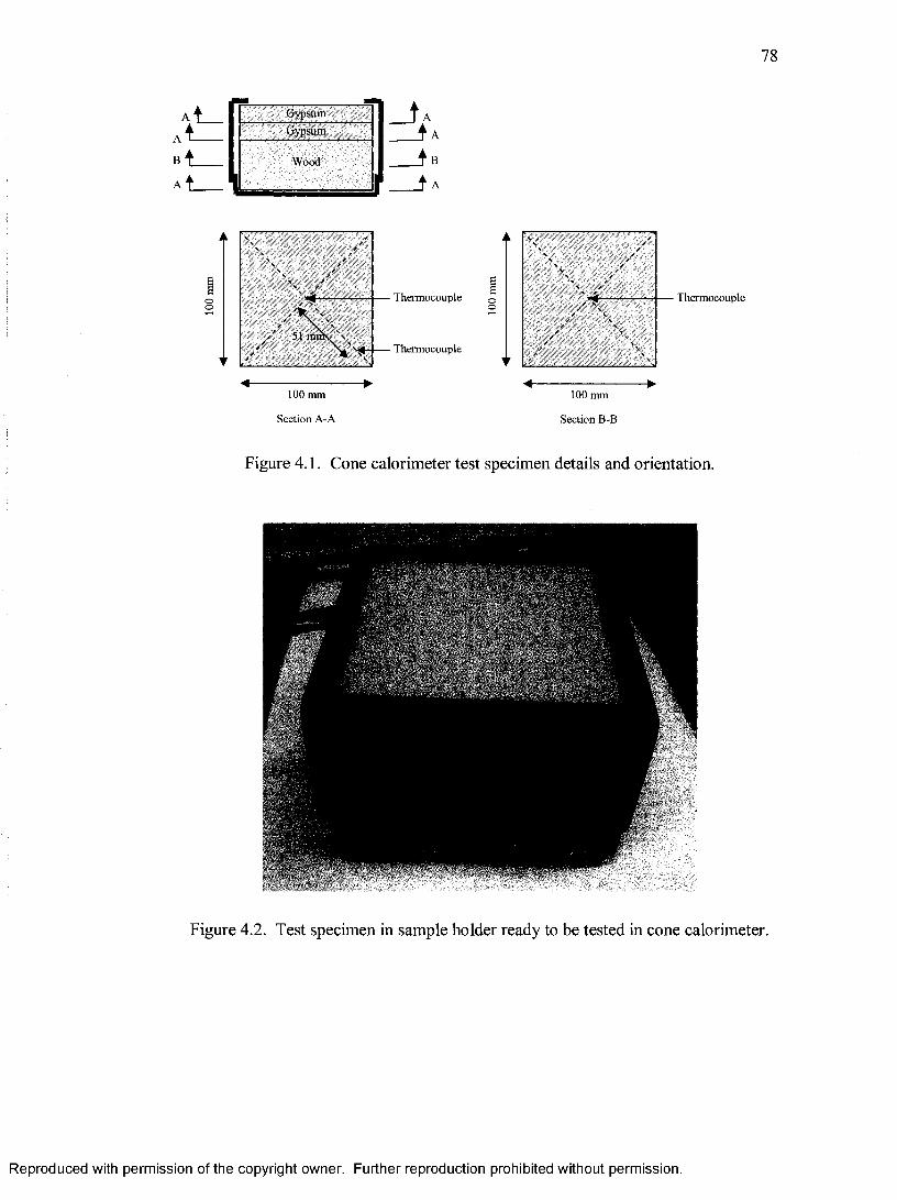
4.1.2. Sample Exposure 79
4.1.3. Test Results 79
4.2. Intermediate and Full-Scale Fire-Resistance Tests 85
4.2.1. Test Assembly 87
4.2.2. Intermediate-scale Fire Resistance Test 88
4.2.2.1. Intermediate- scale Test Assembly 89
4.2.2.2. Intermediate-scale Standard Exposure Test Results 93
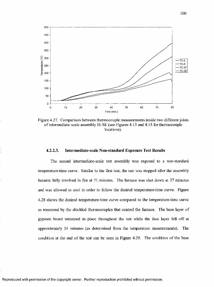
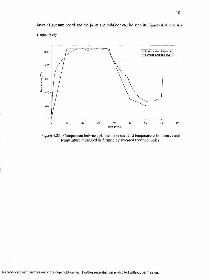
4.2.2.3. Intermediate-scale Non-standard Exposure Test Results 100
4.2.3. Full-scale Fire Resistance Test 109
4.2.3.1. Full-scale Test Assembly 110
4.2.3.2. Full-scale Standard Exposure Test Results 114
4.2.3.3. Full-scale Non-standard Exposure Test Results 121
4.2.4. Comparison between Intermediate and Full-scale Experiments 127
4.3. Summary of Experimental Program 131
5. Model Predictions and Discussion 133
5.1. Cone Calorimeter tests 135
5.2. Intermediate and Full-scale Tests 142
5.2.1. Heat Transfer Boundary Conditions 142
5.2.2. Mass Transfer Boundary Conditions 148
5.2.3. Comparison of Model Predictions to Standard Exposure Experiments.. 148
5.2.4. Comparison of Model Predictions to Full-scale Experiments with Non
standard Exposure 158
5.2.5. Comparison of Model Predictions to Intermediate-scale Experiments with
Non-standard Exposure 162
5.3. Results Summary 165
6. Sensitivity Analysis and Discussion 168
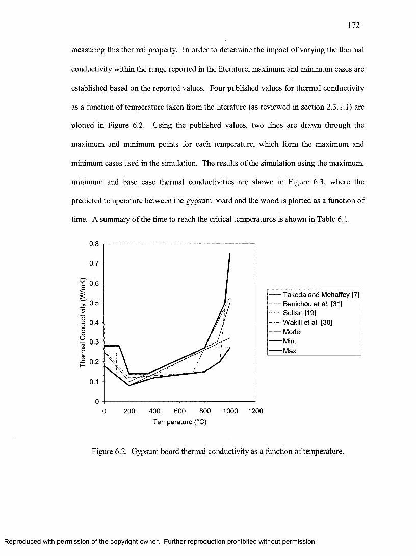
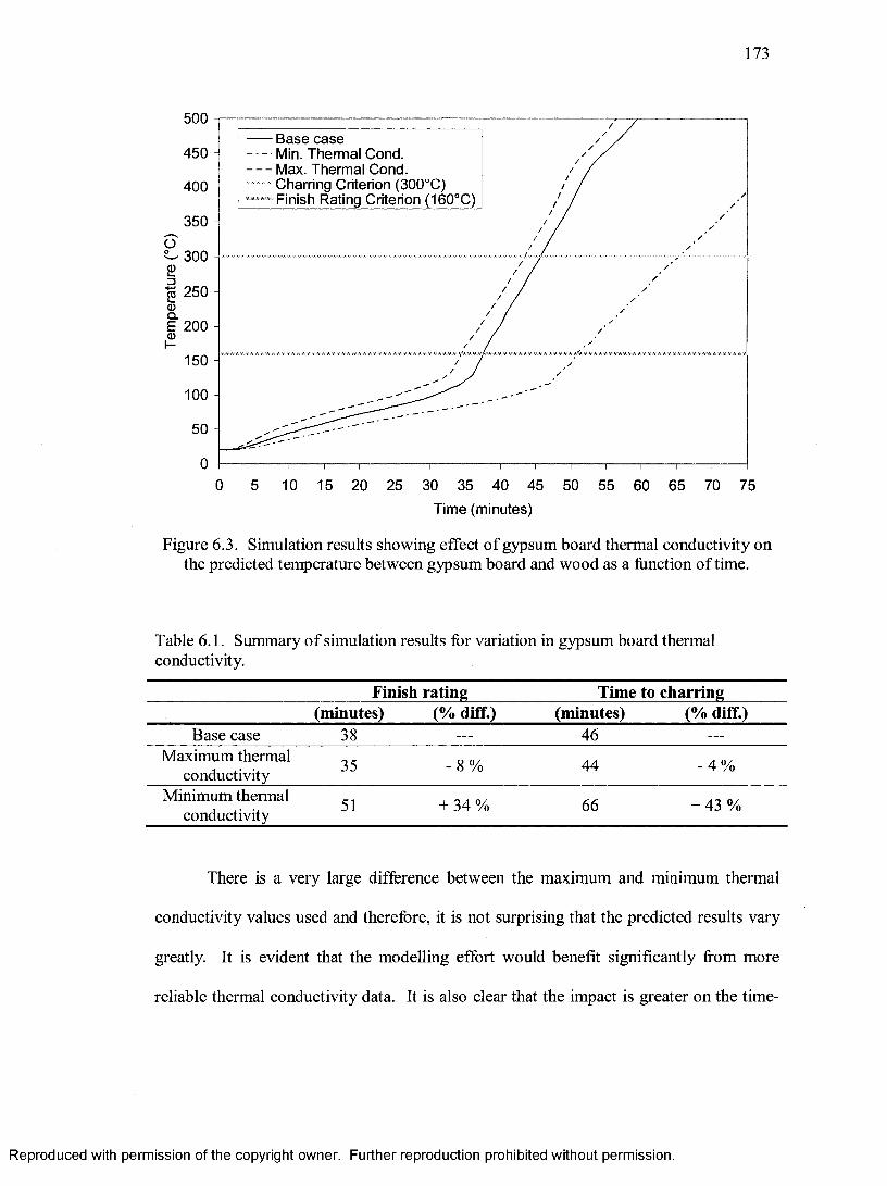
6.1. Impact of Gypsum Board Material Properties 171
6.1.1. Gypsum Board Thermal Conductivity 171
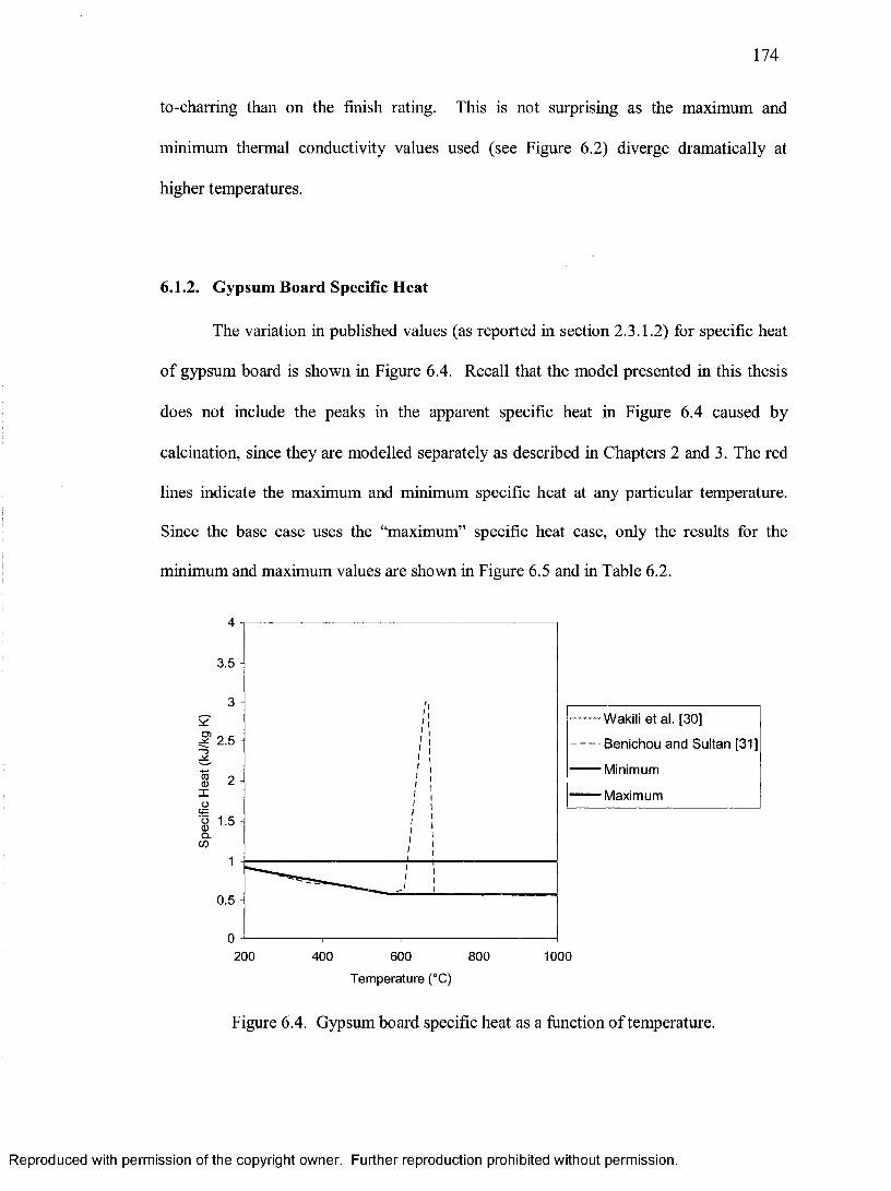
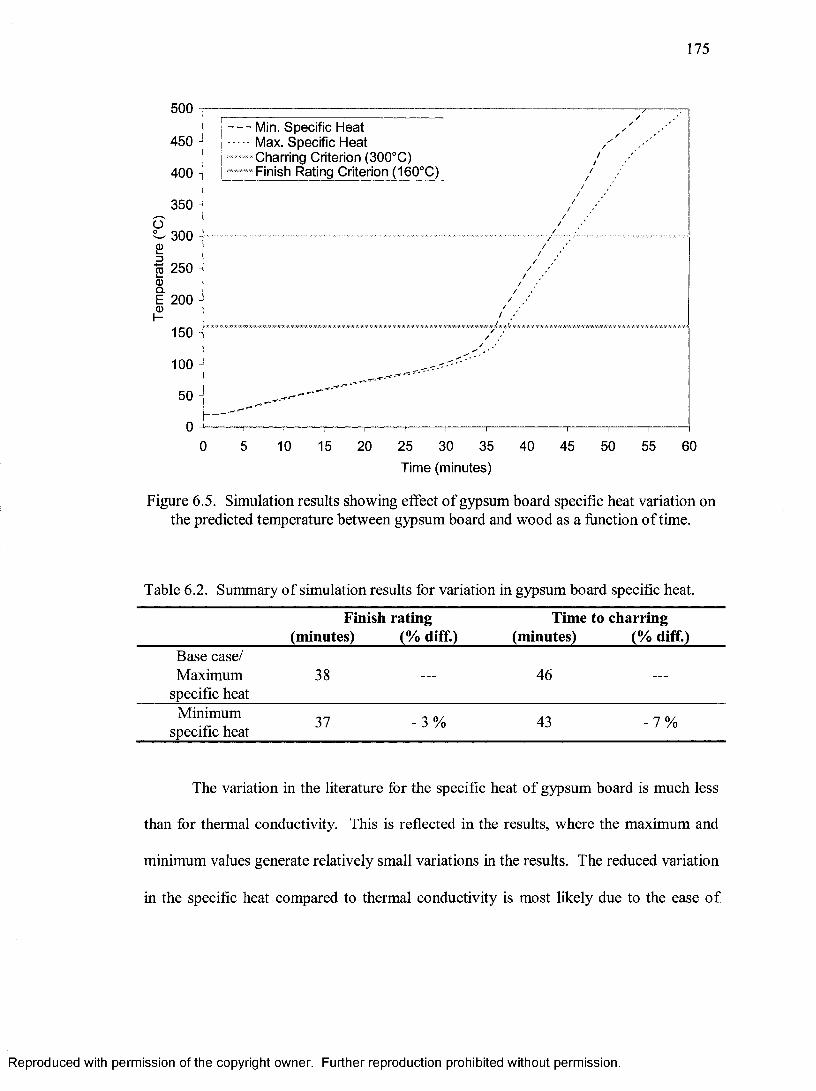
6.1.2. Gypsum Board Specific Heat 174
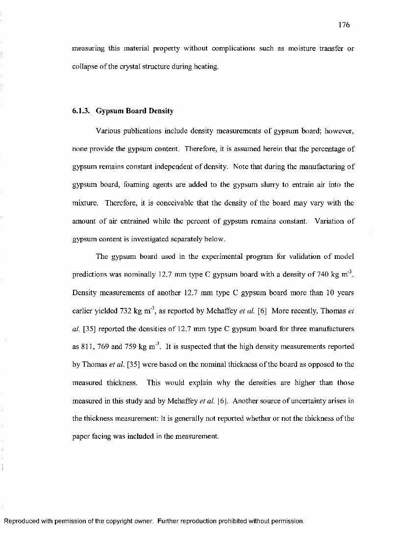
6.1.3. Gypsum Board Density 176
6.1.4. Gypsum Content of Gypsum Board 178
viii
Reproduced with permission of the copyright owner. Further reproduction prohibited without permission.
6.1.5. Gypsum Board Permeability 180
6.2. Impact of Wood Material Properties 182
6.2.1. Wood Thermal Conductivity 182
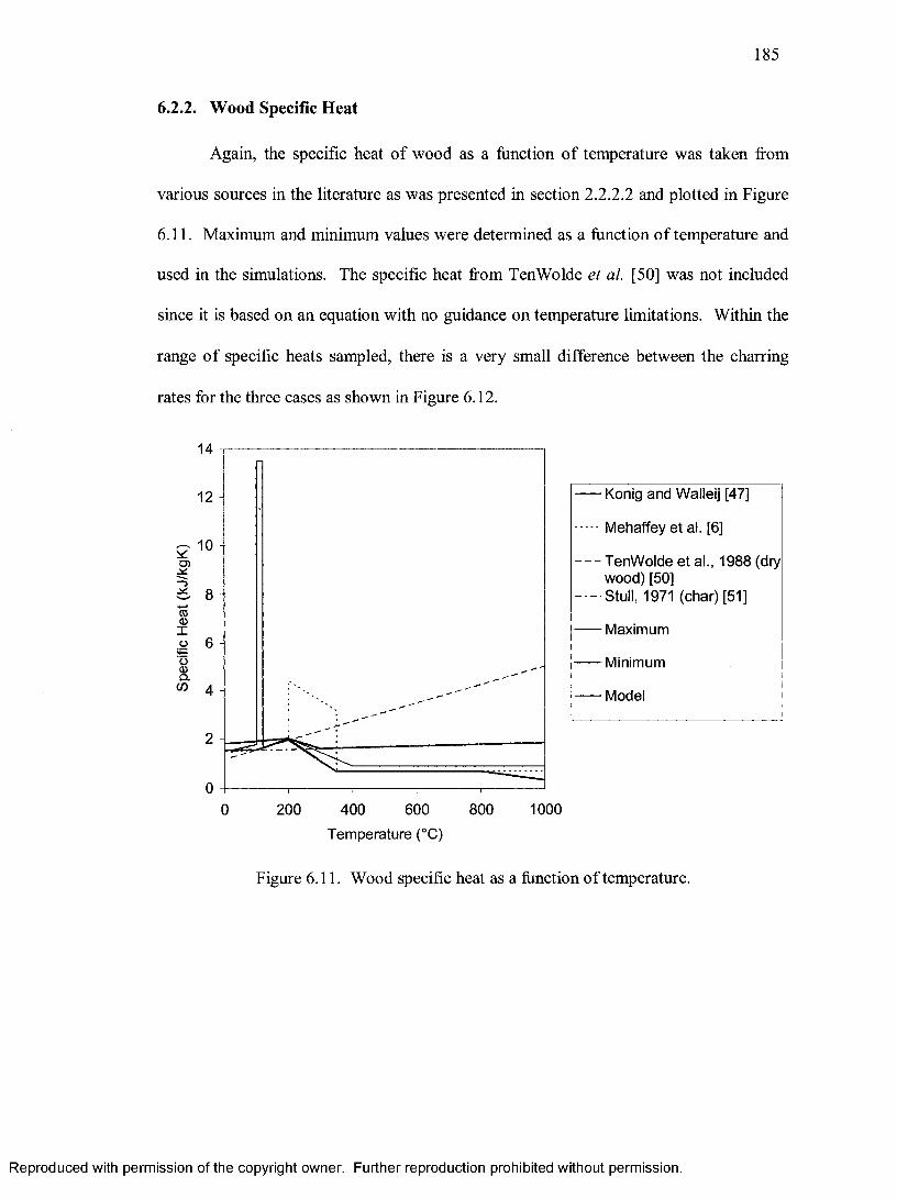
6.2.2. Wood Specific Heat 185
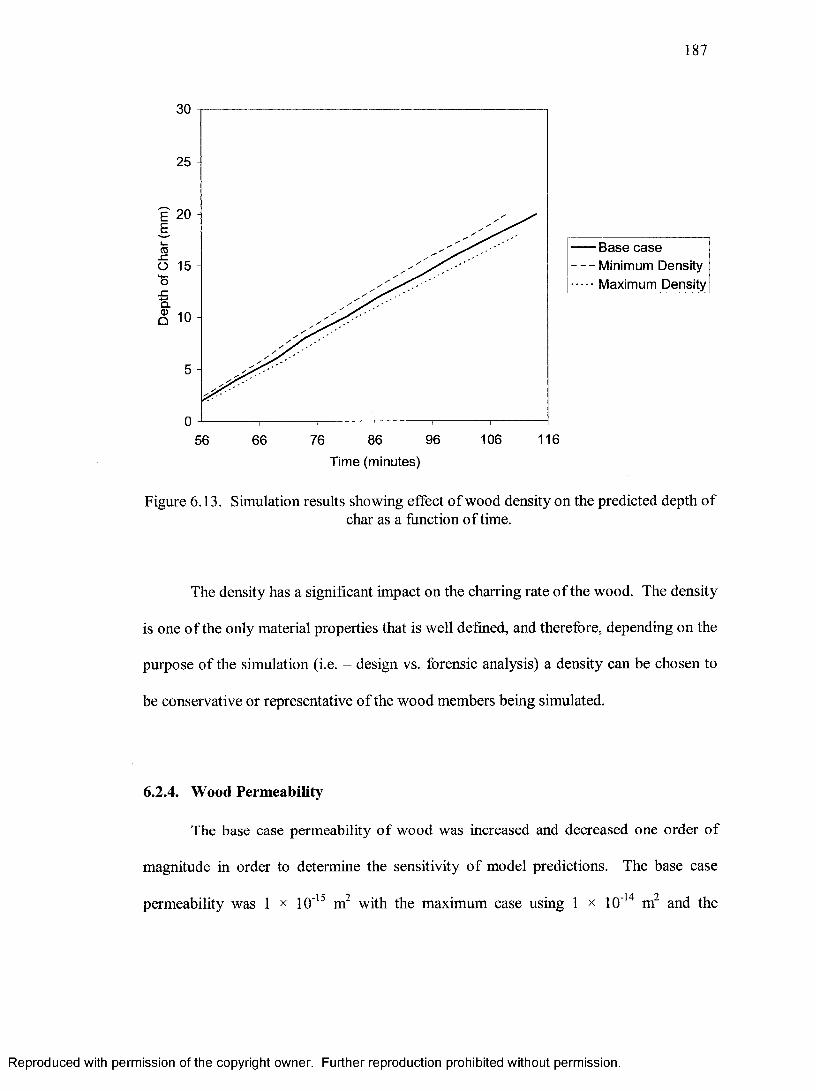
6.2.3. Wood Density 186
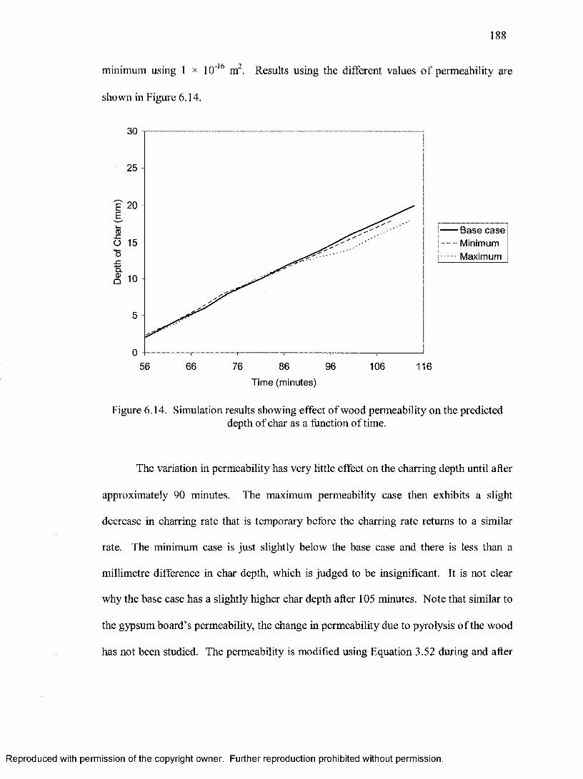
6.2.4. Wood Permeability 187
6.3. Sensitivity Analysis Summary 189
7. Conclusions and Recommendations 192
7.1. Summary 192
7.2. Main Conclusions 194
7.3. Limitations of Model 196
7.4. Contribution 197
7.5. Recommendations for Future Research 197
7.6. Final Remarks 200
References 202
ix
Reproduced with permission of the copyright owner. Further reproduction prohibited without permission.
List of Tables
Table 2.1. Reported gypsum board densities for Canadian fire-rated gypsum board
products 30
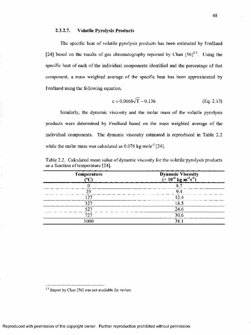
Table 2.2. Calculated mean value of dynamic viscosity for the volatile pyrolysis products
as a function of temperature 48
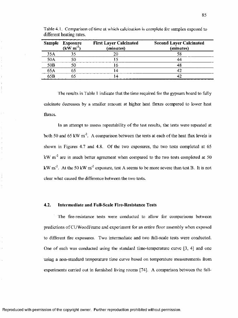
Table 4.1. Comparison of time at which calcination is complete for samples exposed to
different heating rates 85
Table 4.2. Summary of fire-resistance tests completed 87
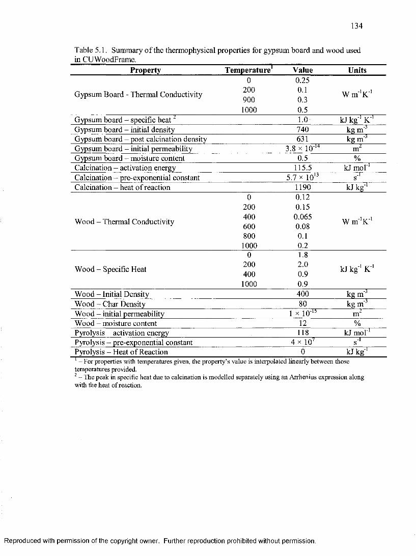
Table 5.1. Summary of the thermophysical properties for gypsum board and wood used
in CUWoodFrame 134
Table 6.1. Summary of simulation results for variation in gypsum board thermal
conductivity 173
Table 6.2. Summary of simulation results for variation in gypsum board specific heat.
175
Table 6.3. Summary of simulation results for variation in gypsum board density 178
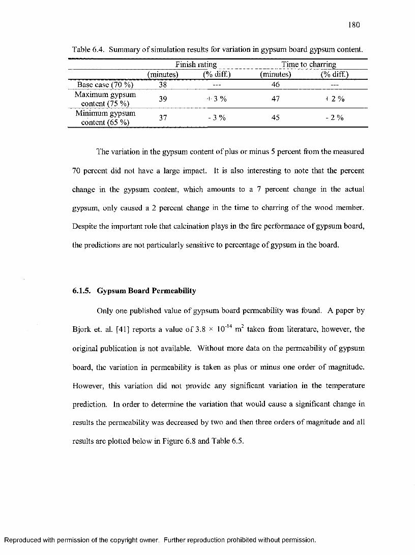
Table 6.4. Summary of simulation results for variation in gypsum board gypsum content.
180
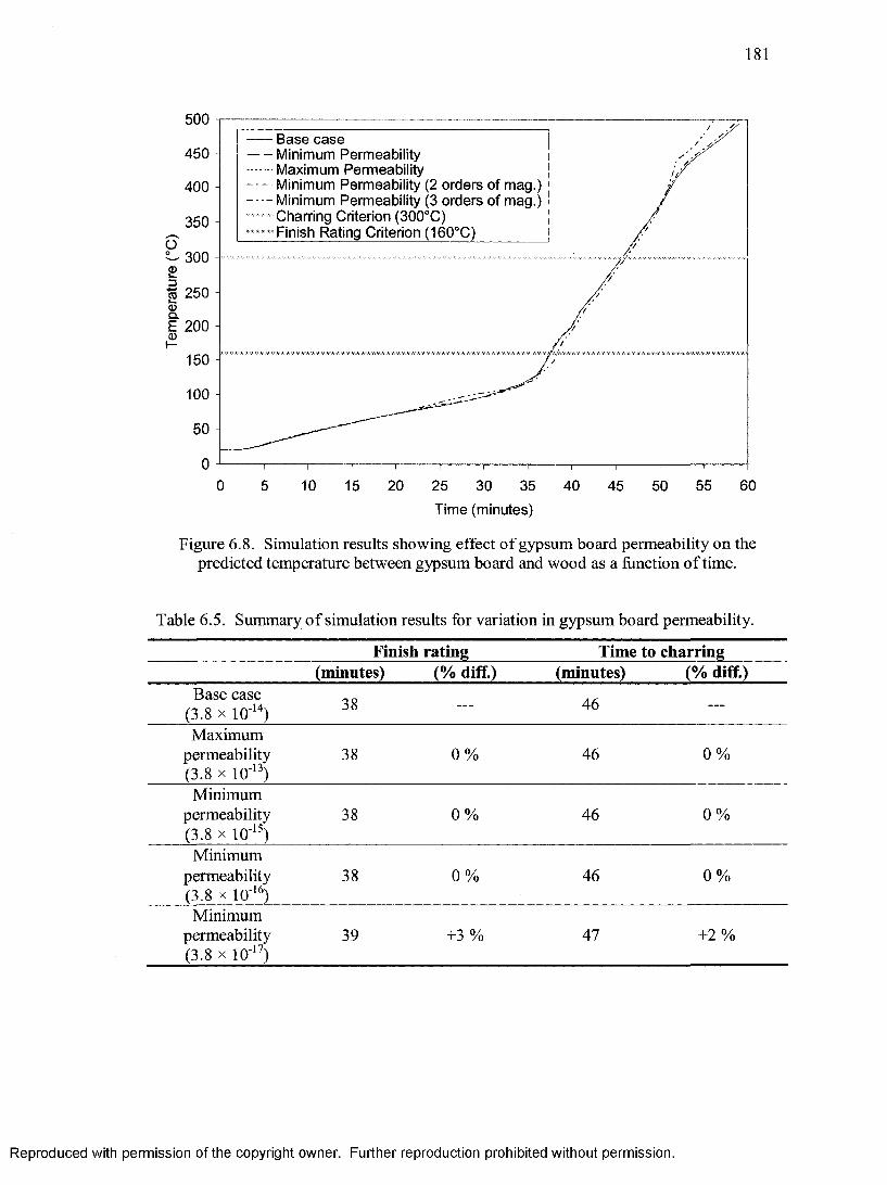
Table 6.5. Summary of simulation results for variation in gypsum board permeability.
181
Table 6.6. Summary of impact of each gypsum board parameter on the time to charring
of the protected wood 189
Table 6.7. Summary of impact of each wood parameter on char depth 189
x
Reproduced with permission of the copyright owner. Further reproduction prohibited without permission.
List of Figures
Figure 2.1. Typical floor furnace 7
Figure 2.2. Temperature exposure as a function of time in the standard fire-resistance
test, CAN/ULC S101 8
Figure 2.3. Thermal conductivity of gypsum board as a function of temperature 26
Figure 2.4. Specific heat of gypsum board as a function of temperature 29
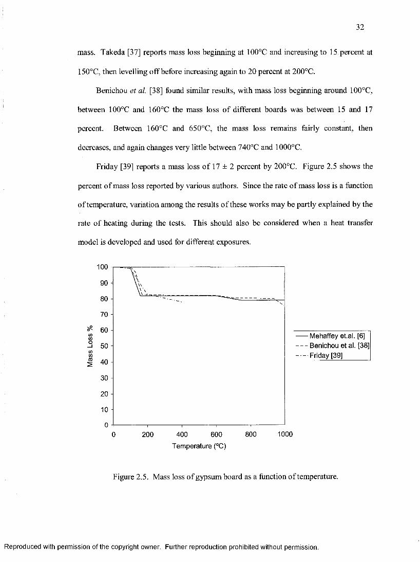
Figure 2.5. Mass loss of gypsum board as a function of temperature 32
Figure 2.6. Comparison of mass loss between four different gypsum board products.... 33
Figure 2.7. Comparison between mass loss of gypsum board at three different heating
rates 34
Figure 2.8. Shrinkage in gypsum board as a function of temperature up to 500 °C 37
Figure 2.9. Shrinkage in gypsum board as a function of temperature up to 1000°C 37
Figure 2.10. Degradation of wood by low-temperature and high-temperature pathways.
40
Figure 2.11. Thermal conductivity of wood as a function of temperature 42
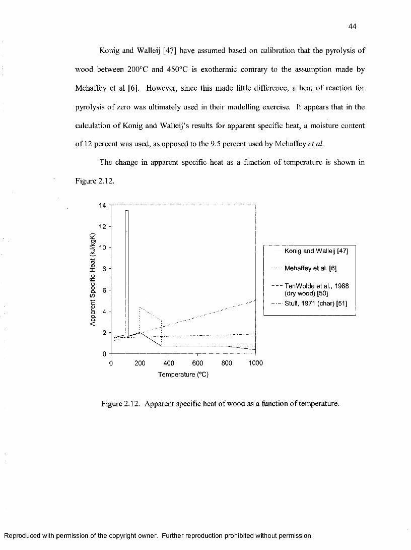
Figure 2.12. Apparent specific heat of wood as a function of temperature 44
Figure 3.1. Cross-section of floor assembly to be analyzed in the heat and mass transfer
model taking advantage of symmetry 53
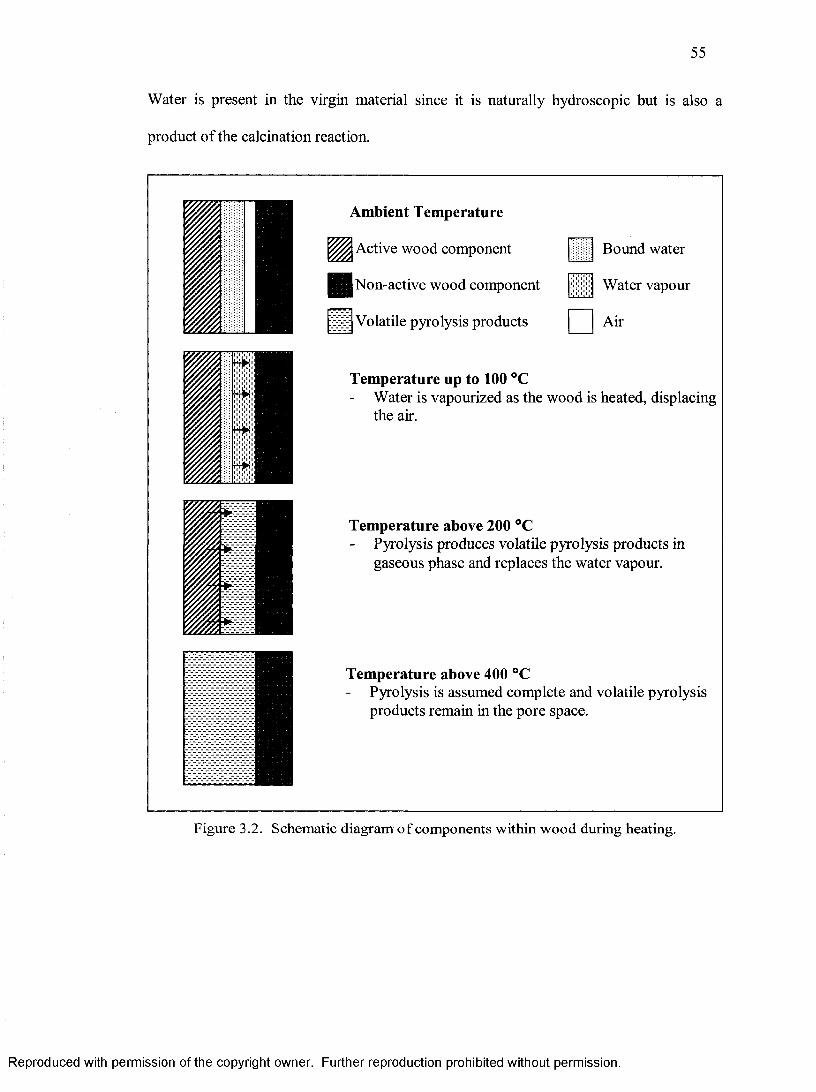
Figure 3.2. Schematic diagram of components within wood during heating 55
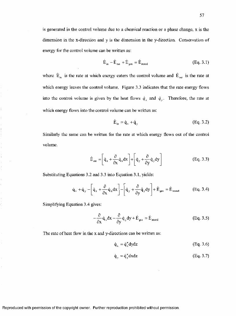
Figure 3.3. Two-dimensional control volume for heat transfer 56
Figure 3.4. Two-dimensional control volume for mass 66
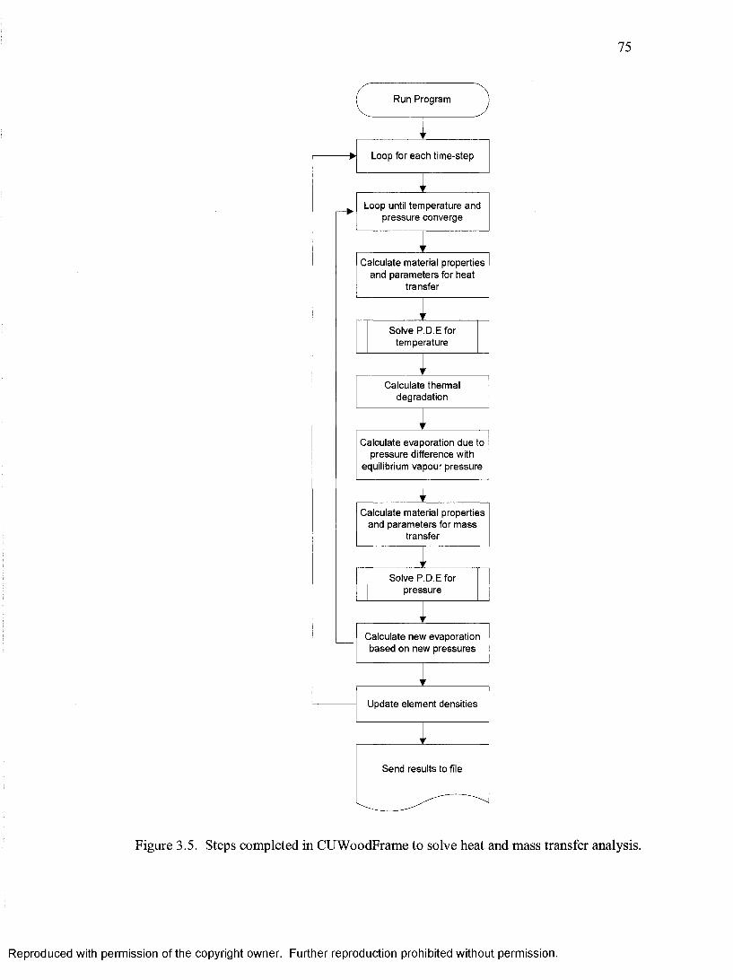
Figure 3.5. Steps completed in CUWoodFrame to solve heat and mass transfer analysis.
75
Figure 4.1. Cone calorimeter test specimen details and orientation 78
Figure 4.2. Test specimen in sample holder ready to be tested in cone calorimeter 78
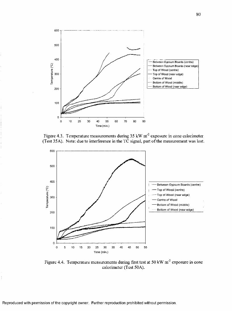
Figure 4.3. Temperature measurements during 35 kW m"2 exposure in cone calorimeter.
80
Figure 4.4. Temperature measurements during first test at 50 kW m"2 exposure in cone
calorimeter 80
XI
Reproduced with permission of the copyright owner. Further reproduction prohibited without permission.
Figure 4.5. Temperature measurements during second test at 50 kW m"2 exposure in cone
calorimeter 81
Figure 4.6. Temperature measurements during first test at 65 kW m"2 exposure in cone
calorimeter 81
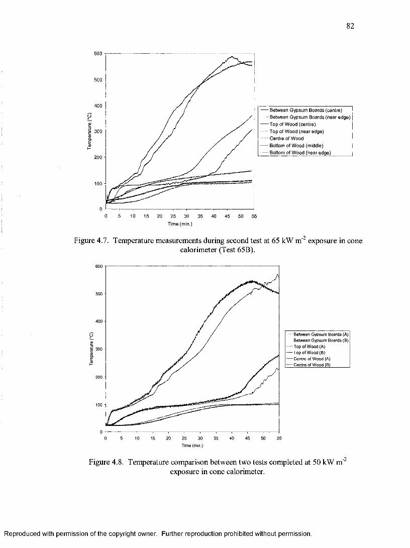
Figure 4.7. Temperature measurements during second test at 65 kW m"2 exposure in cone
calorimeter 82
Figure 4.8. Temperature comparison between two tests completed at 50 kW m"2
exposure in cone calorimeter 82
Figure 4.9. Temperature comparison between two tests completed at 65 kW m"2
exposure in cone calorimeter 83
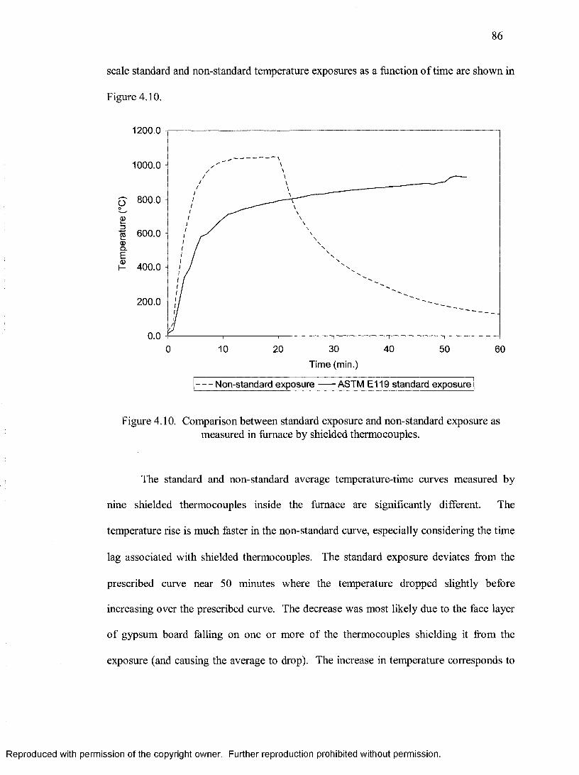
Figure 4.10. Comparison between standard exposure and non-standard exposure as
measured in furnace by shielded thermocouples 86
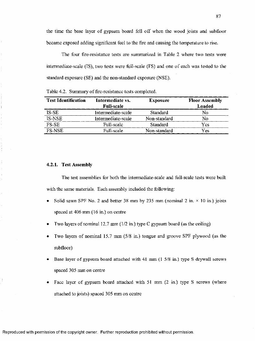
Figure 4.11. Assembly IS-SE placed on intermediate-scale furnace at beginning of test.
89
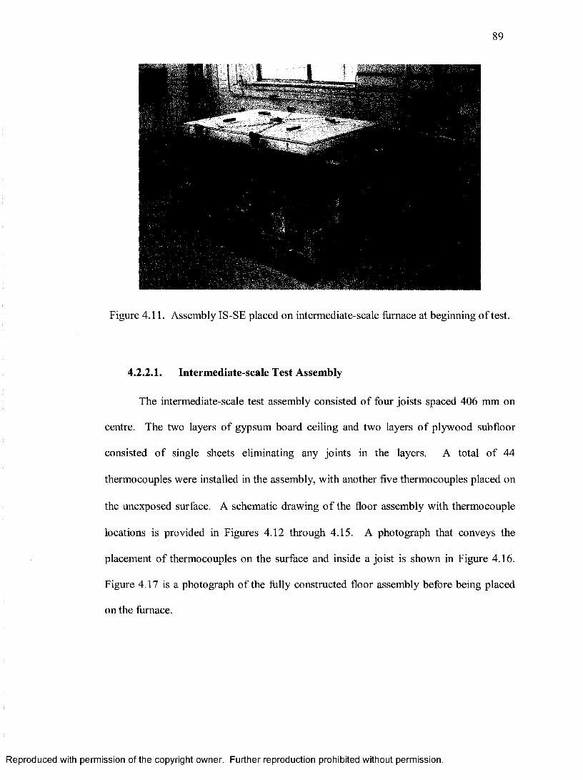
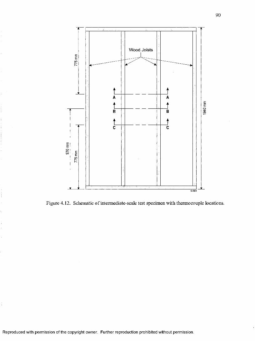
Figure 4.12. Schematic of intermediate-scale test specimen with thermocouple locations.
90
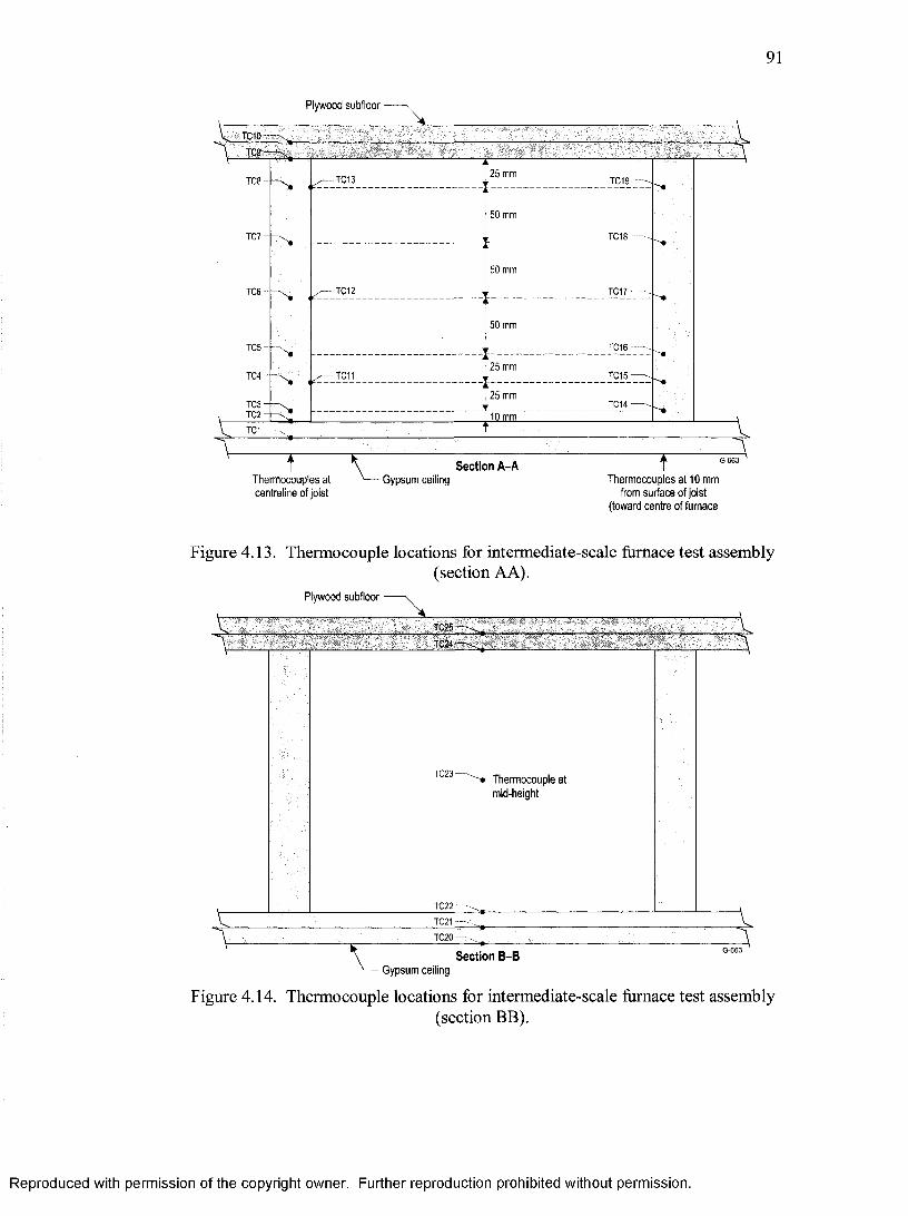
Figure 4.13. Thermocouple locations for intermediate-scale furnace test assembly
(section AA) 91
Figure 4.14. Thermocouple locations for intermediate-scale furnace test assembly
(section BB) 91
Figure 4.15. Thermocouple locations for intermediate-scale furnace test assembly
(section CC) 92
Figure 4.16. Thermocouples placed on surface and at mid-depth of joist in assembly
IS-SE 92
Figure 4.17. Assembly IS-SE ready to be tested (placed with ceiling facing up in
photograph) 93
Figure 4.18. Assembly IS-SE after test exposure and before being lifted off furnace 95
Figure 4.19. Exposed side of assembly IS-SE after test and extinguishment 95
Figure 4.20. Side view of assembly IS-SE after test and extinguishment 95
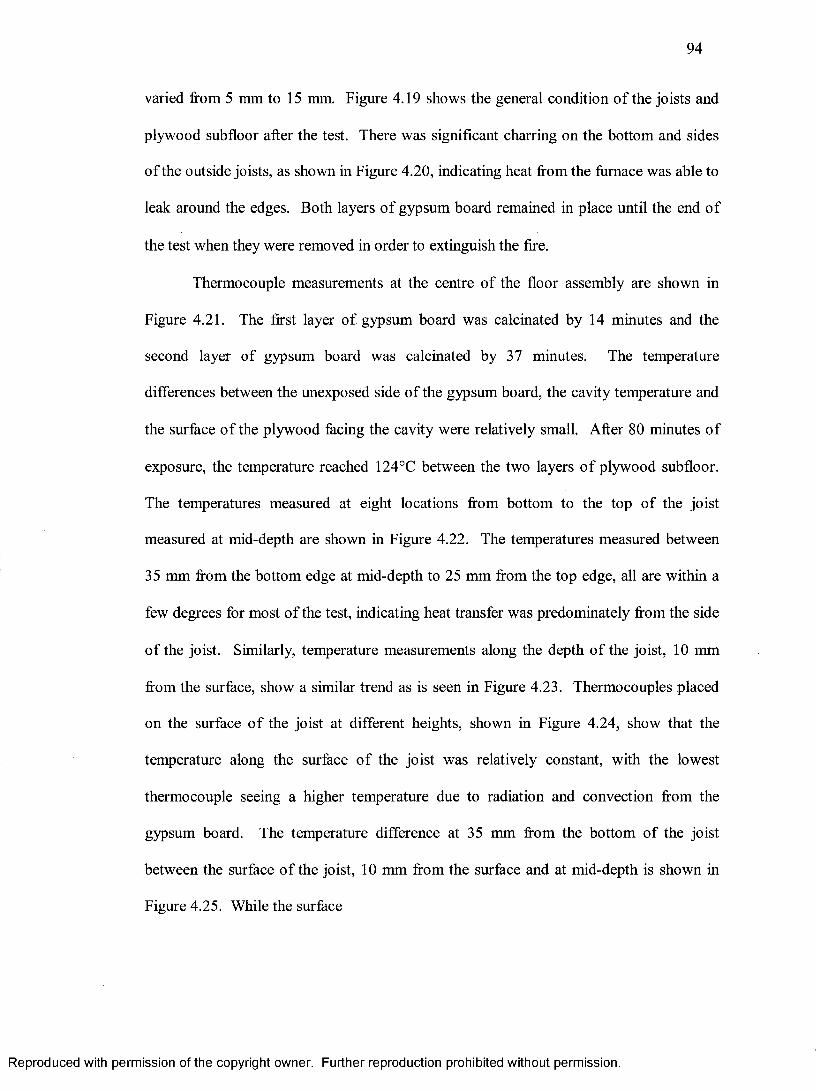
Figure 4.21. Thermocouple measurements at centre of intermediate-scale assembly
IS-SE 97
xii
Reproduced with permission of the copyright owner. Further reproduction prohibited without permission.
Figure 4.22. Thermocouple measurements at various depths inside mid-depth of joist of
intermediate-scale assembly IS-SE 97
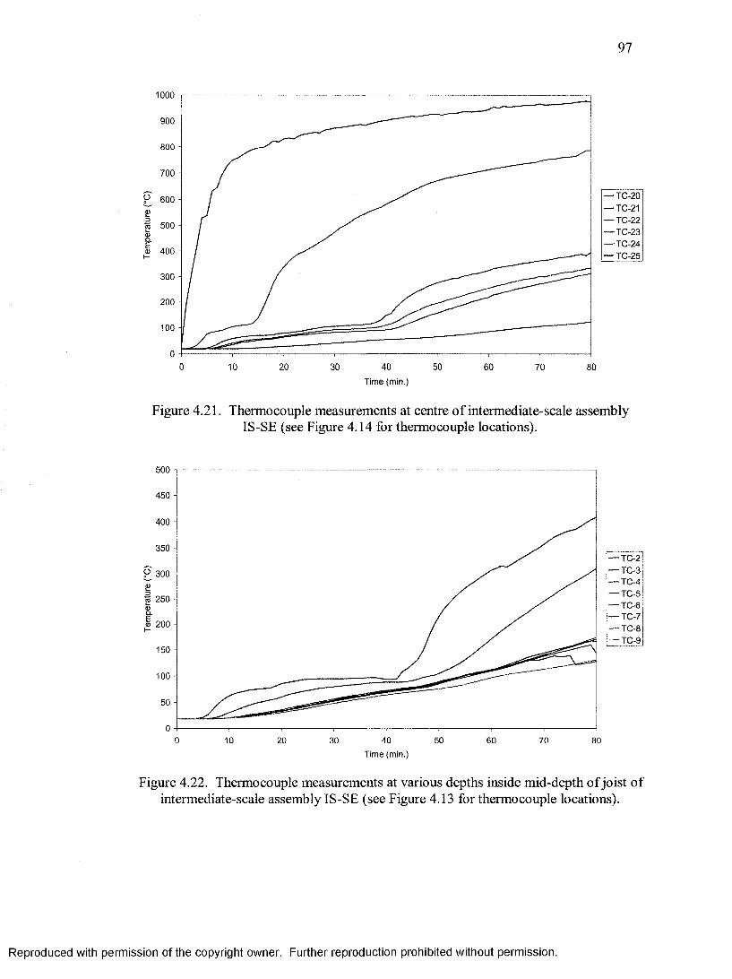
Figure 4.23. Thermocouple measurements at various depths inside joist 10 mm from
surface of intermediate-scale assembly IS-SE 98
Figure 4.24. Thermocouple measurements along surface of joist facing centre cavity of
intermediate-scale assembly IS-SE 98
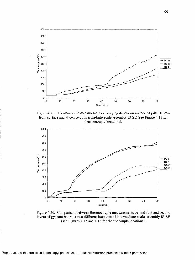
Figure 4.25. Thermocouple measurements at varying depths on surface of joist, 10 mm
from surface and at centre of intermediate-scale assembly IS-SE 99
Figure 4.26. Comparison between thermocouple measurements behind first and second
layers of gypsum board at two different locations of intermediate-scale assembly IS-
SE 99
Figure 4.27. Comparison between thermocouple measurements inside two different joists
of intermediate-scale assembly IS-SE 100
Figure 4.28. Comparison between planned non-standard temperature-time curve and
temperature measured in furnace by shielded thermocouples 101
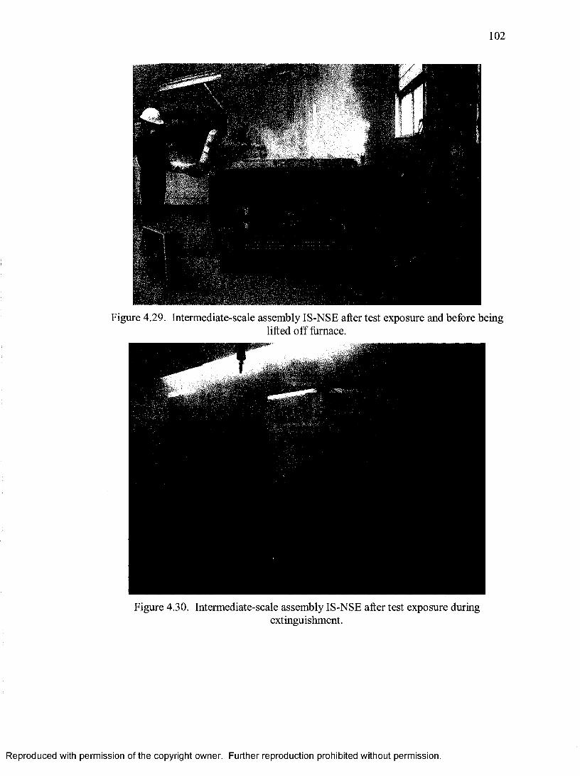
Figure 4.29. Intermediate-scale assembly IS-NSE after test exposure and before being
lifted off furnace 102
Figure 4.30. Intermediate-scale assembly IS-NSE after test exposure during
extinguishment 102
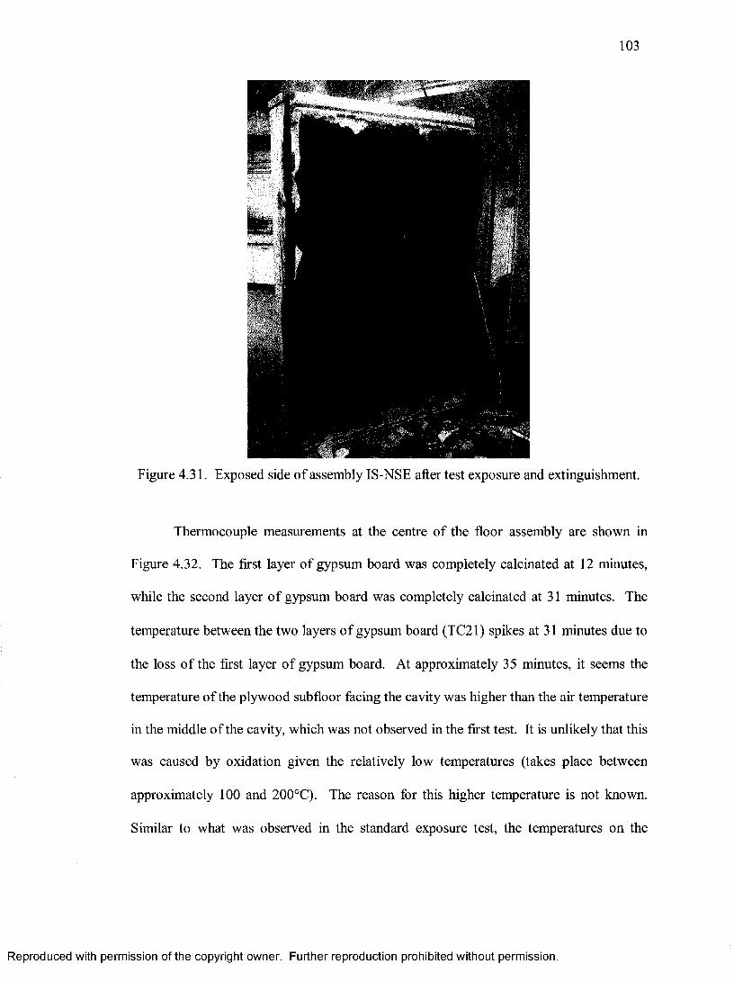
Figure 4.31. Exposed side of assembly IS-NSE after test exposure and extinguishment.
103
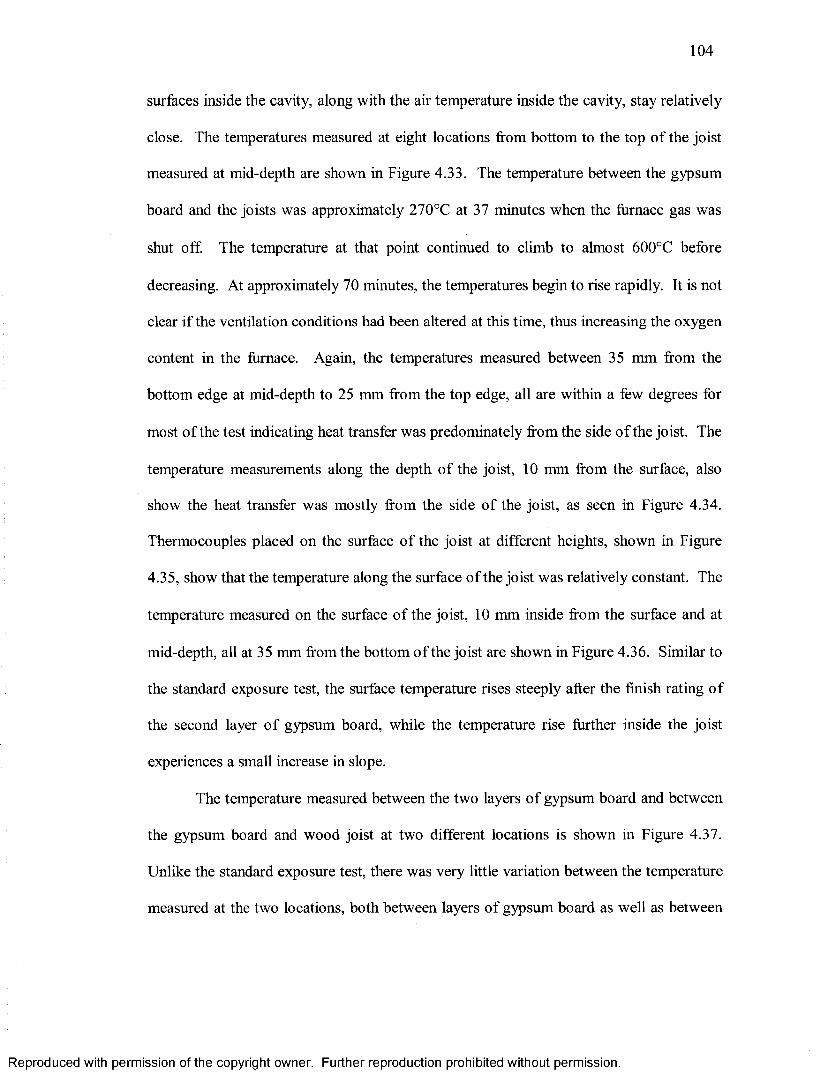
Figure 4.32. Thermocouple measurements at centre of intermediate-scale assembly IS-
NSE 105
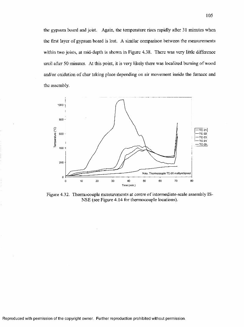
Figure 4.33. Thermocouple measurements at various depths inside mid-depth of joist of
intermediate-scale assembly IS-NSE 106
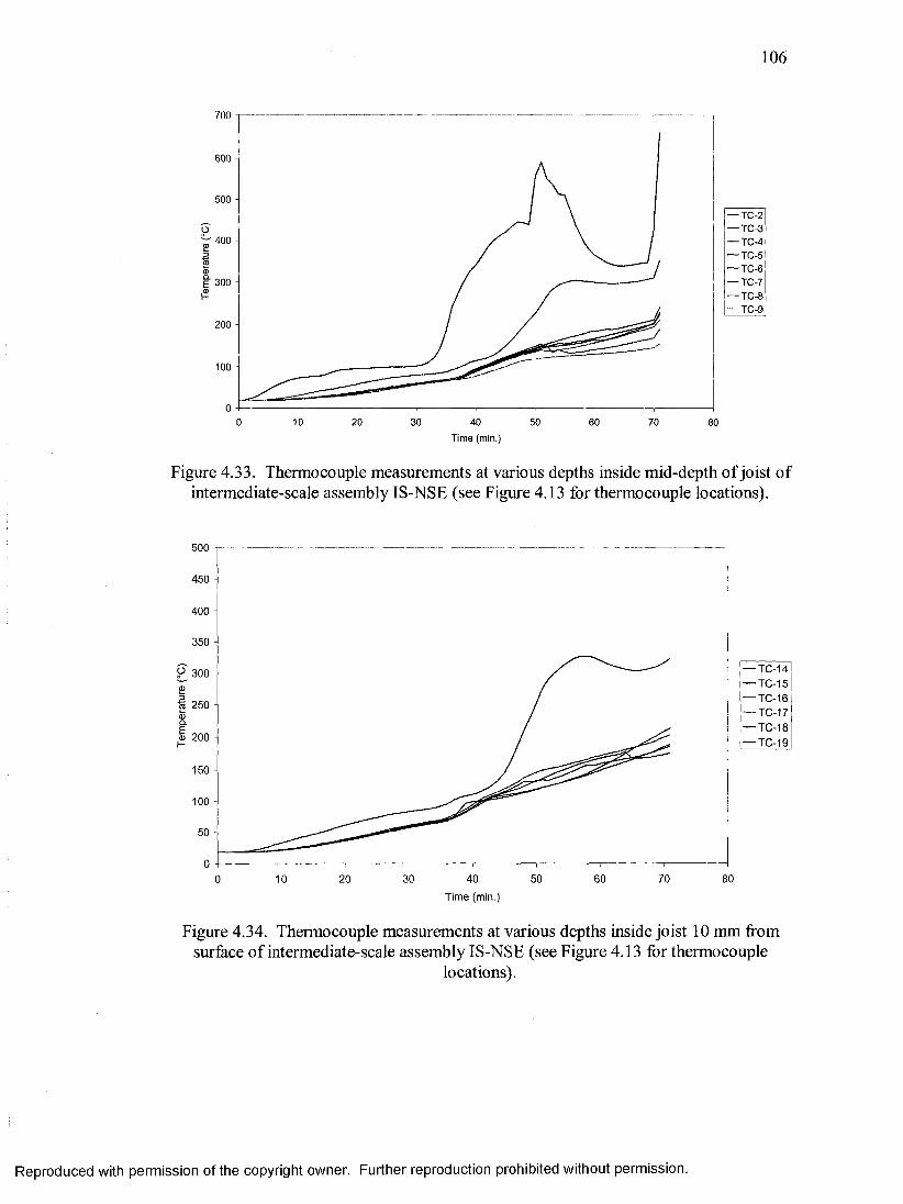
Figure 4.34. Thermocouple measurements at various depths inside joist 10 mm from
surface of intermediate-scale assembly IS-NSE 106
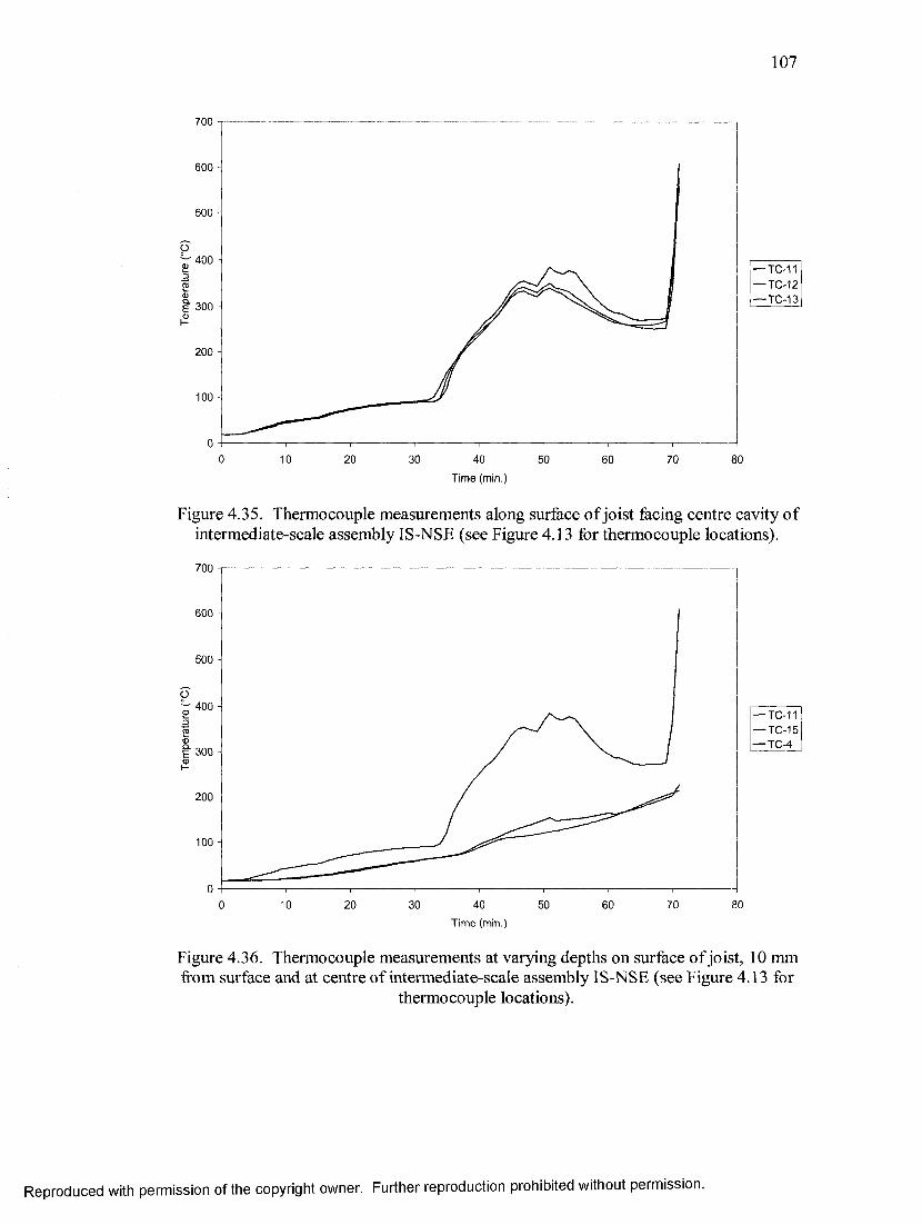
Figure 4.35. Thermocouple measurements along surface of joist facing centre cavity of
intermediate-scale assembly IS-NSE 107
Figure 4.36. Thermocouple measurements at varying depths on surface of joist, 10 mm
from surface and at centre of intermediate-scale assembly IS-NSE 107
xm
Reproduced with permission of the copyright owner. Further reproduction prohibited without permission.
Figure 4.37. Comparison between thermocouple measurements behind first and second
layers of gypsum board, at two different locations, in intermediate-scale assembly IS-
NSE 108
Figure 4.38. Comparison between thermocouple measurements inside two different joists
of intermediate-scale assembly IS-NSE 108
Figure 4.39. Full-scale fire-resistance floor furnace at the NRCC 109
Figure 4.40. Loading mechanism on the full-scale fire-resistance floor furnace at the
NRCC 109
Figure 4.41. Full-scale floor assembly during construction in test frame 110
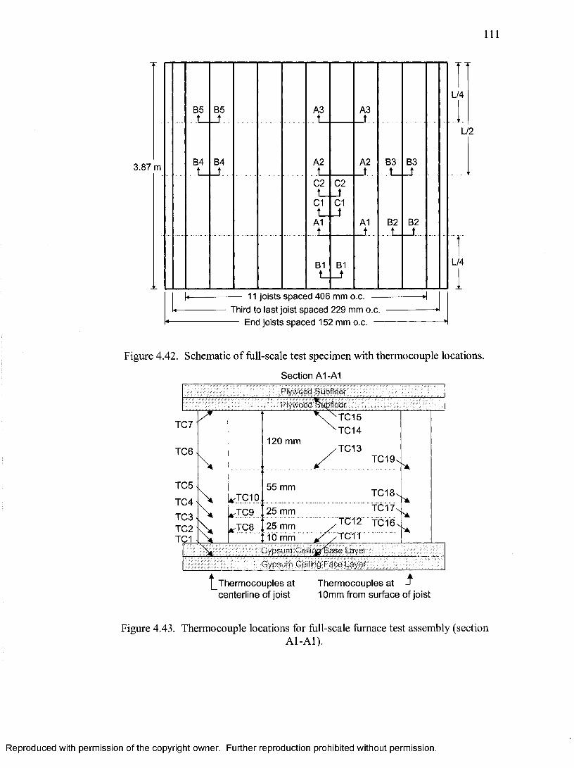
Figure 4.42. Schematic of full-scale test specimen with thermocouple locations Ill
Figure 4.43. Thermocouple locations for full-scale furnace test assembly (section
Al-Al) Ill
Figure 4.44. Thermocouple locations for full-scale furnace test assembly (section
A2-A2) 112
Figure 4.45. Thermocouple locations for full-scale furnace test assembly (section
A3-A3)
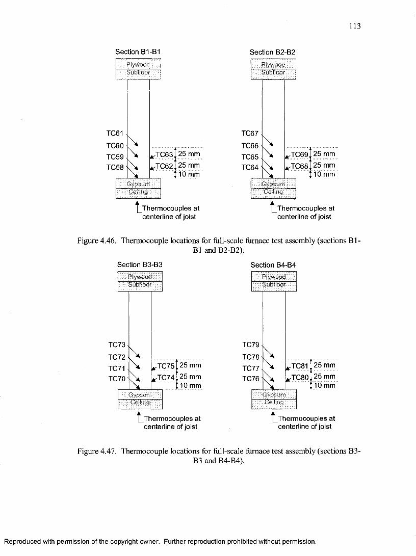
Figure 4.46. Thermocouple locations for full-scale furnace test assembly (sections B1
B1 and B2-B2)
112
113
Figure 4.47. Thermocouple locations for full-scale furnace test assembly (sections B3-
B3 and B4-B4) 113
Figure 4.48. Thermocouple locations for full-scale furnace test assembly (sections B5-
B5, Cl-Cl and C2-C2) 114
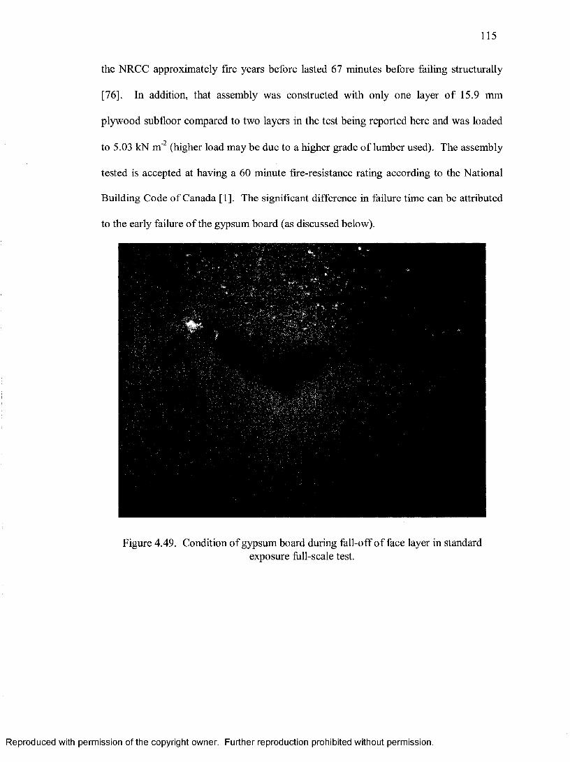
Figure 4.49. Condition of gypsum board during fall-off of face layer in standard
exposure full-scale test 115
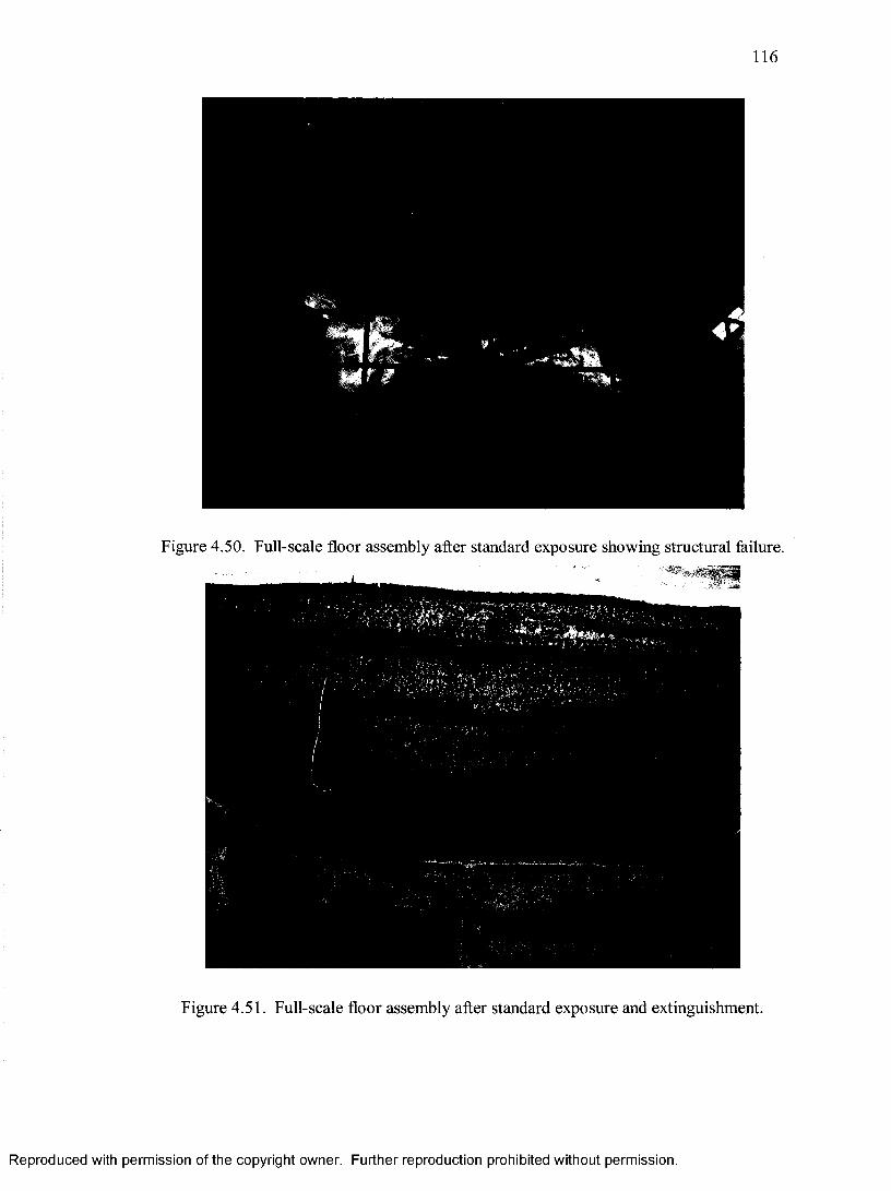
Figure 4.50. Full-scale floor assembly after standard exposure showing structural failure.
116
Figure 4.51. Full-scale floor assembly after standard exposure and extinguishment.... 116
Figure 4.52. Top view of full-scale floor assembly after standard exposure 117
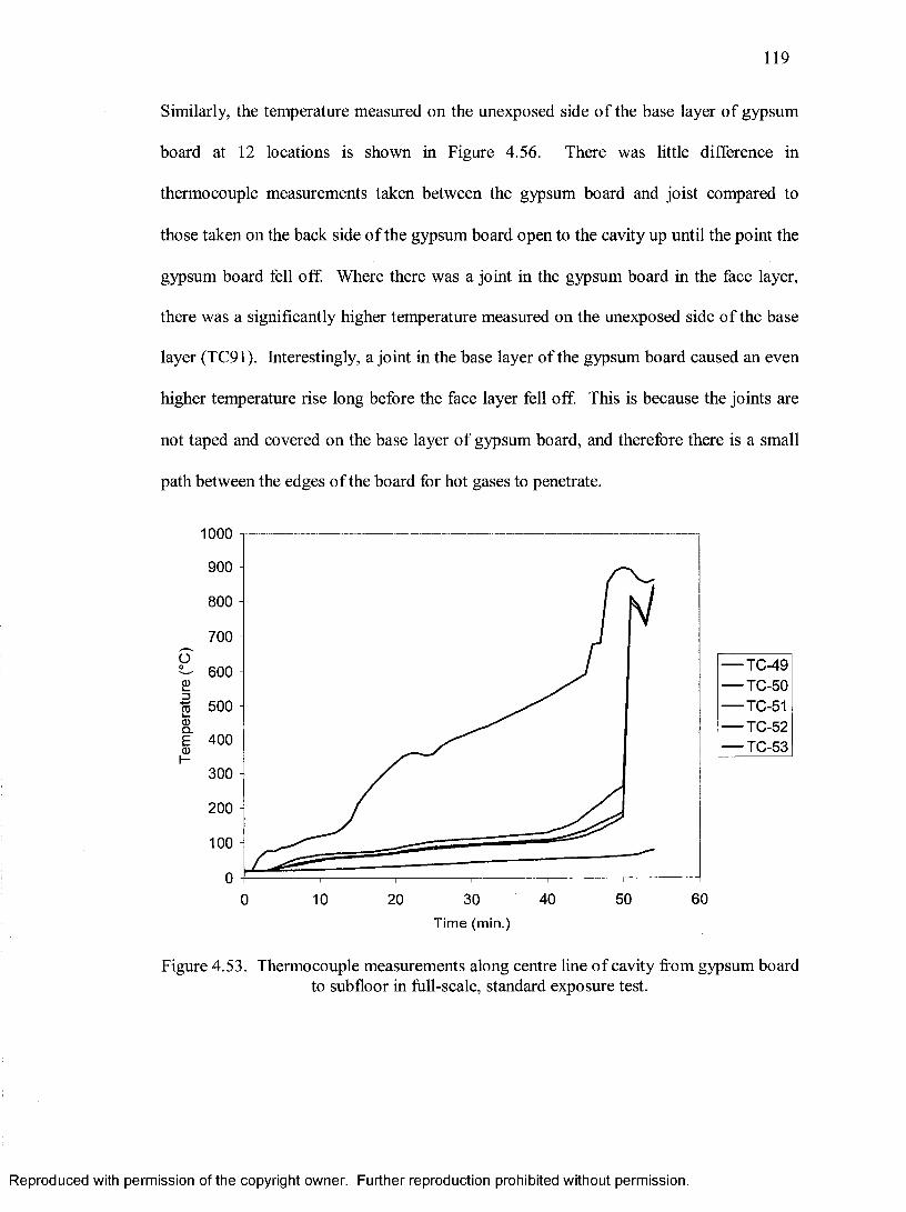
Figure 4.53. Thermocouple measurements along centre line of cavity from gypsum board
to subfloor in full-scale, standard exposure test 119
xiv
Reproduced with permission of the copyright owner. Further reproduction prohibited without permission.
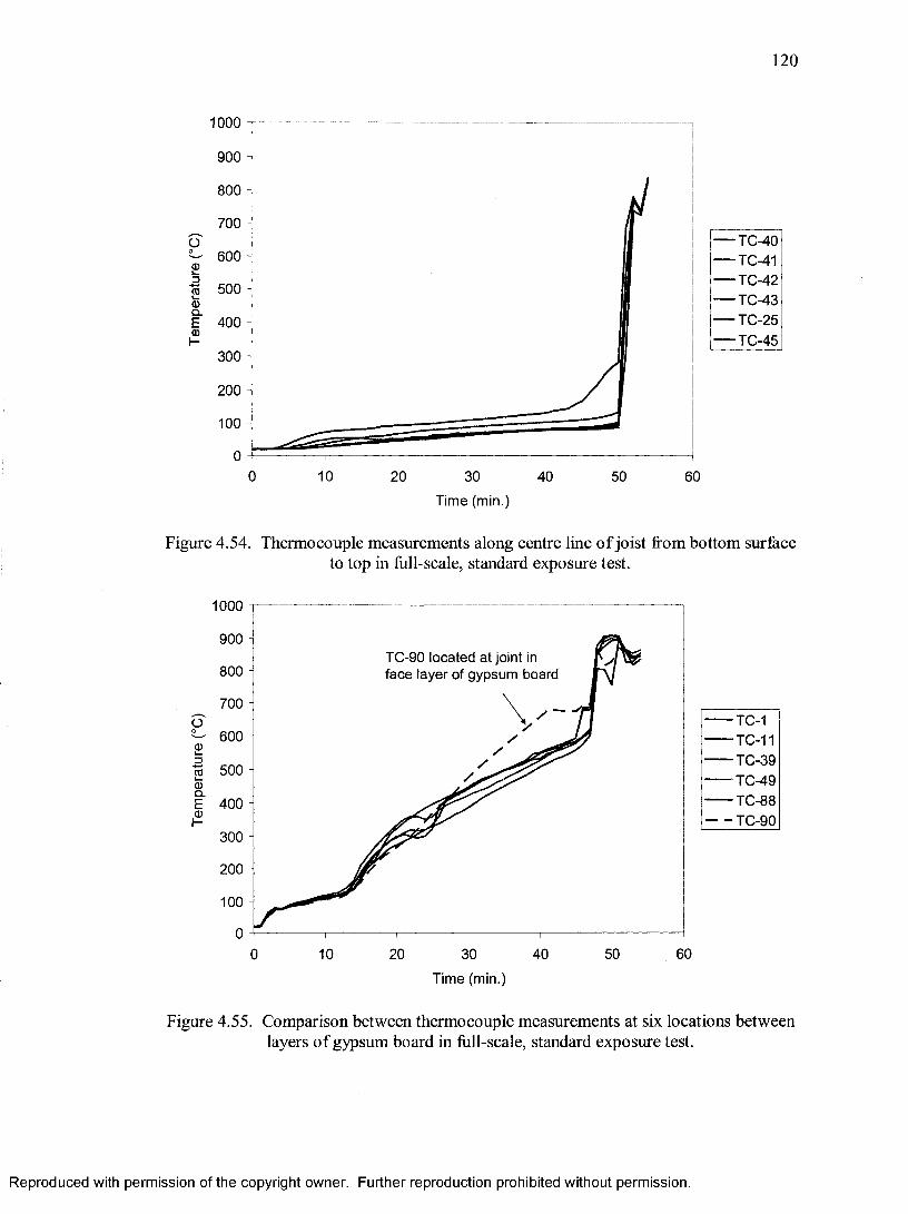
Figure 4.54. Thermocouple measurements along centre line of joist from bottom surface
to top in full-scale, standard exposure test 120
Figure 4.55. Comparison between thermocouple measurements at six locations between
layers of gypsum board in full-scale, standard exposure test 120
Figure 4.56. Comparison between thermocouple measurements at 12 locations on the
unexposed face of the base layer of gypsum board (both between joist and gypsum
board and facing cavity) in full-scale, standard exposure test 121
Figure 4.57. Full-scale floor assembly after non-standard exposure 122
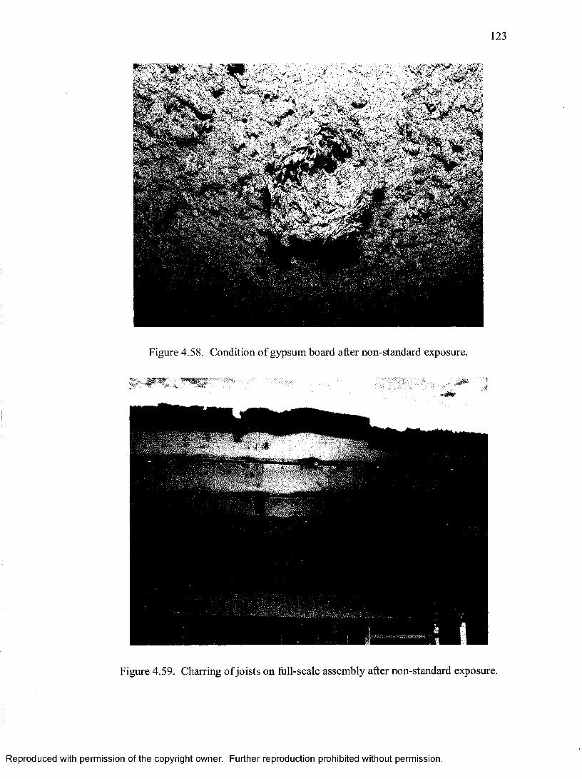
Figure 4.58. Condition of gypsum board after non-standard exposure 123
Figure 4.59. Charring of joists on full-scale assembly after non-standard exposure 123
Figure 4.60. Thermocouple measurements along centre line of cavity from gypsum board
to subfloor in full-scale, non-standard exposure test 125
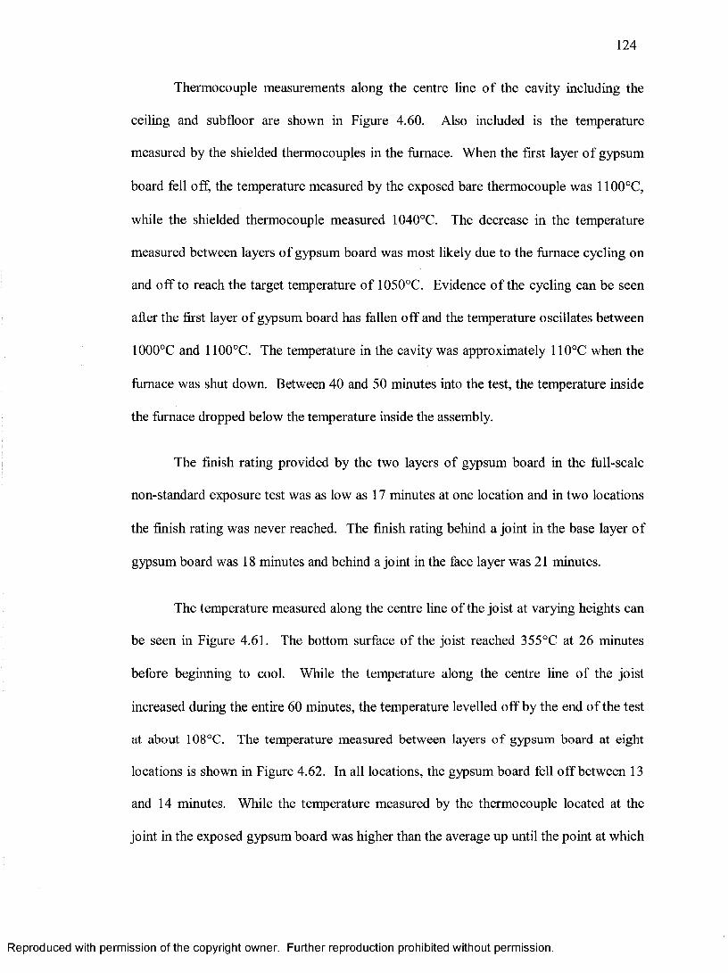
Figure 4.61. Thermocouple measurements along centre line of joist from bottom surface
to top in full-scale, non-standard exposure test 126
Figure 4.62. Comparison between thermocouple measurements at six locations between
layers of gypsum board in full-scale, non-standard exposure test 126
Figure 4.63. Comparison between thermocouple measurements at 12 locations on the
unexposed face of the base layer of gypsum board (both between joist and gypsum
board and facing cavity) in full-scale, non-standard exposure test 127
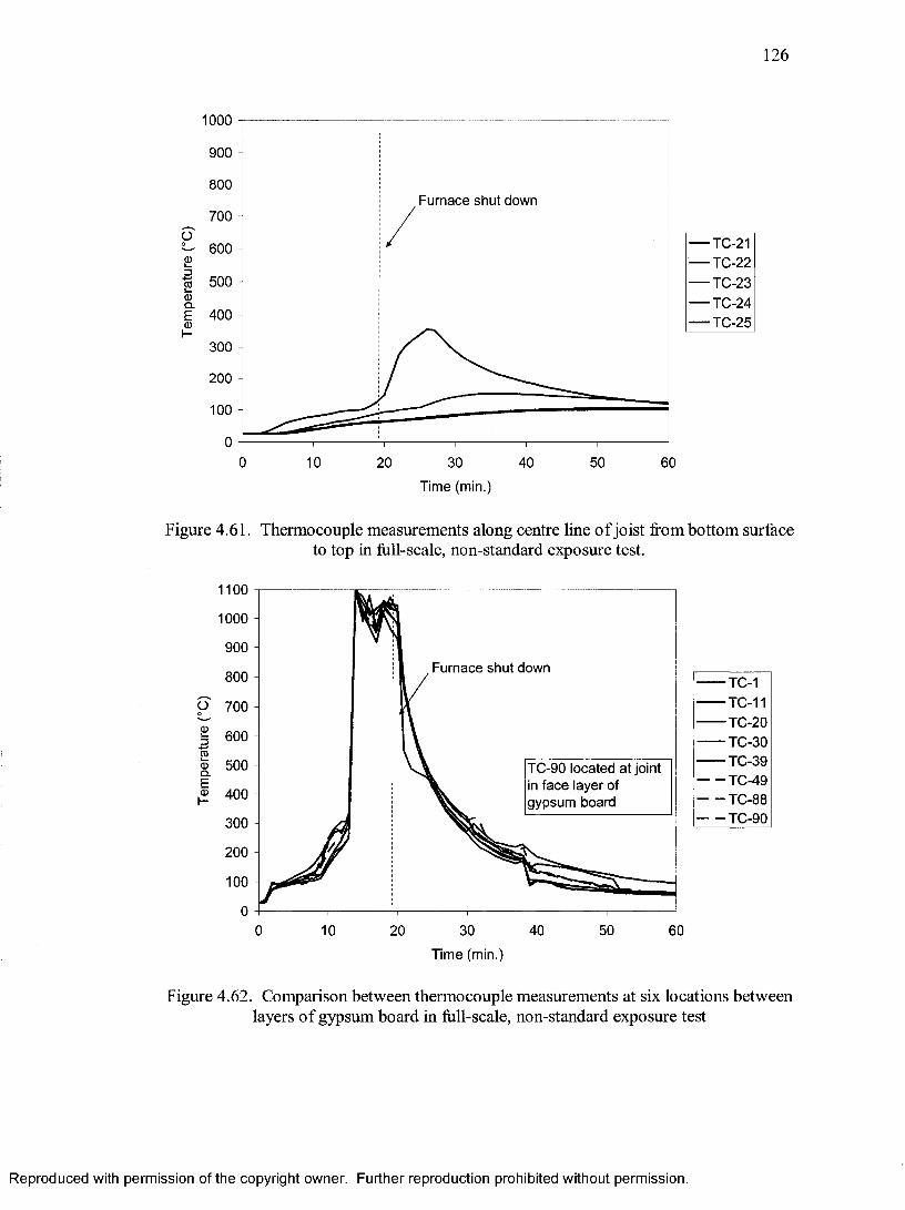
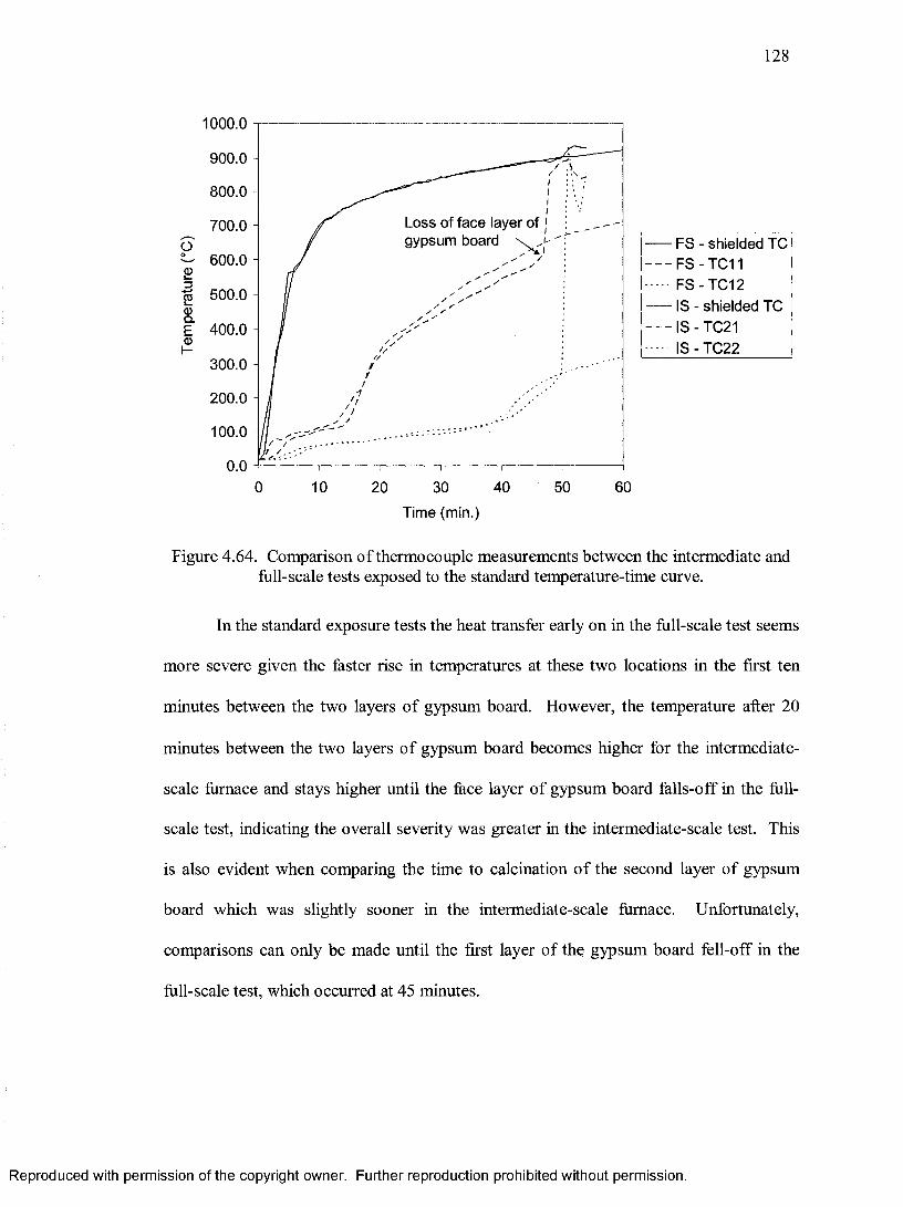
Figure 4.64. Comparison of thermocouple measurements between the intermediate and
full-scale tests exposed to the standard temperature-time curve 128
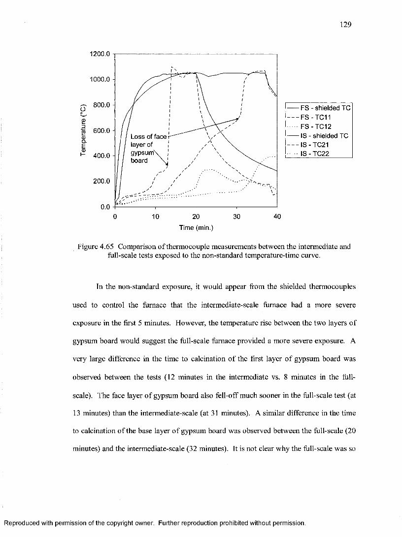
Figure 4.65 Comparison of thermocouple measurements between the intermediate and
full-scale tests exposed to the non-standard temperature-time curve 129
Figure 5.1. Finite element mesh used to model cone calorimeter experiments 136
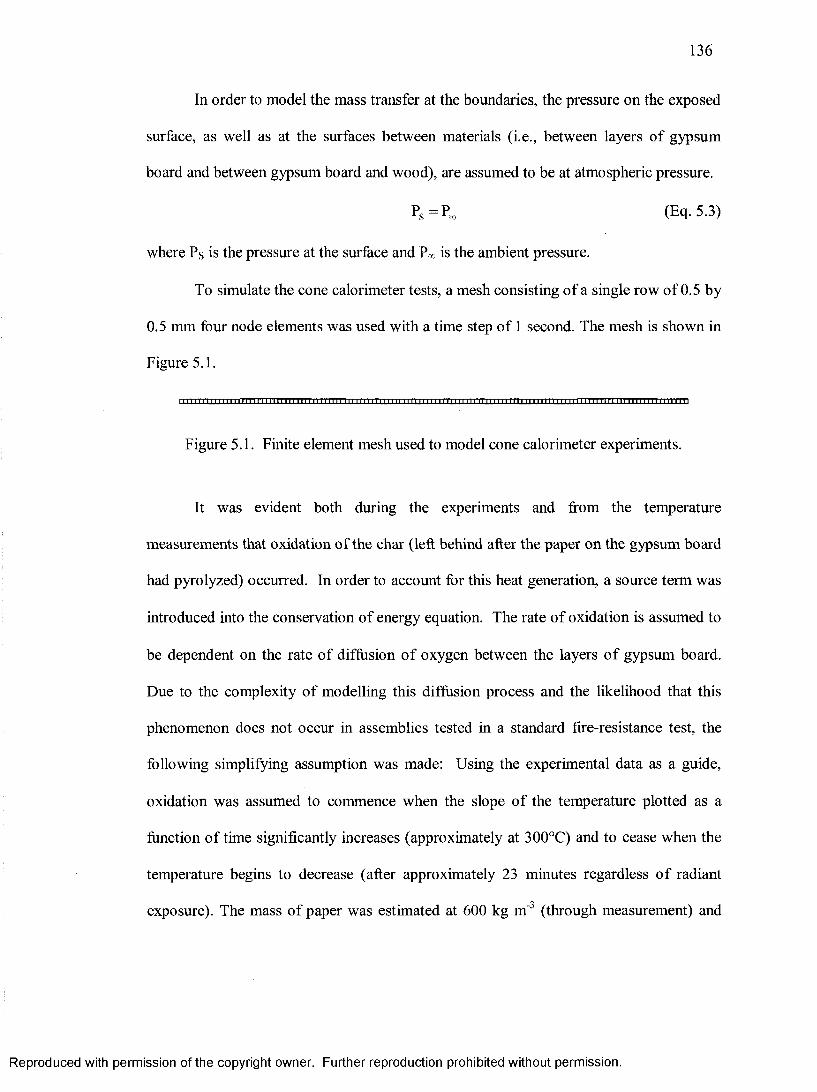
Figure 5.2. Comparison between experiment and model predictions of temperature for 35
kW m'2 exposure 138
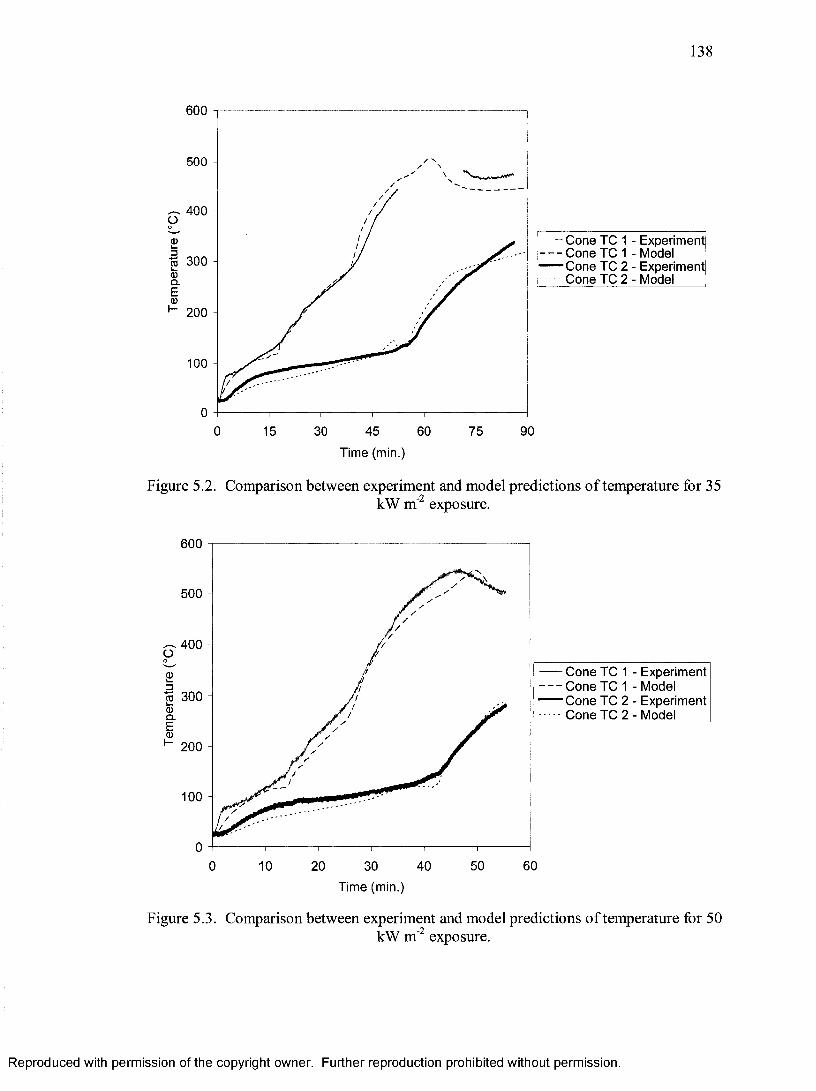
Figure 5.3. Comparison between experiment and model predictions of temperature for 50
kW m~2 exposure 138
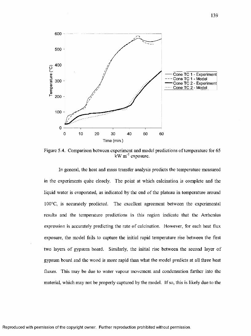
Figure 5.4. Comparison between experiment and model predictions of temperature for 65
kW m"2 exposure 139
xv
Reproduced with permission of the copyright owner. Further reproduction prohibited without permission.
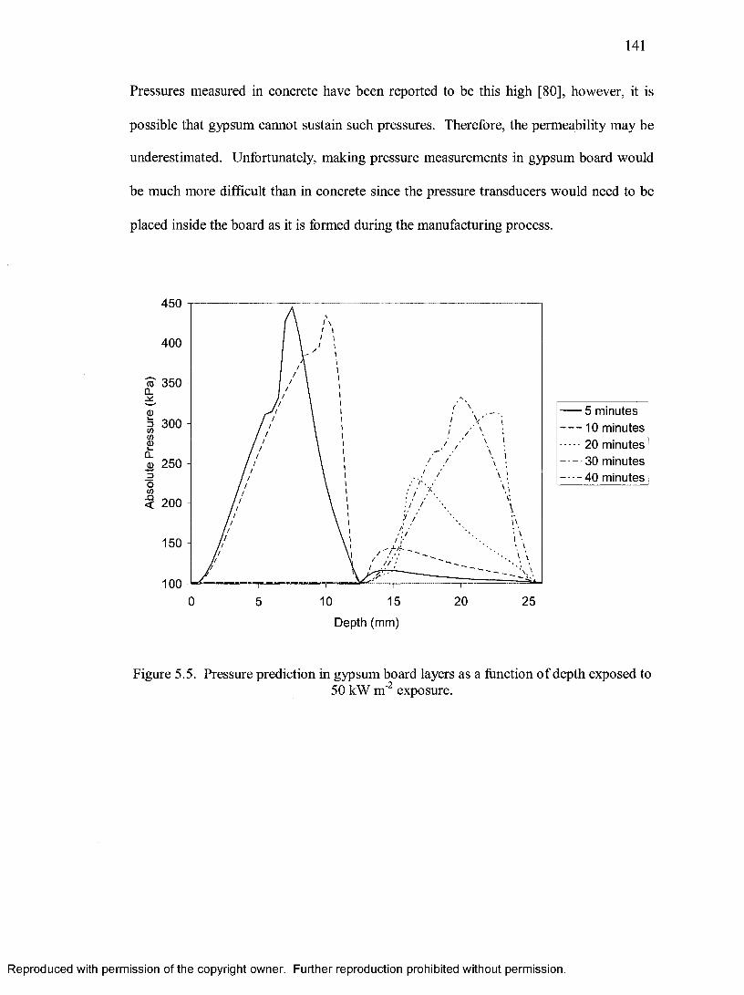
Figure 5.5. Pressure prediction in gypsum board layers as a function of depth exposed to
50 kW m"2 exposure 141
Figure 5.6. Mesh generated by ConFepv for modelling intermediate and full-scale
experiments 145
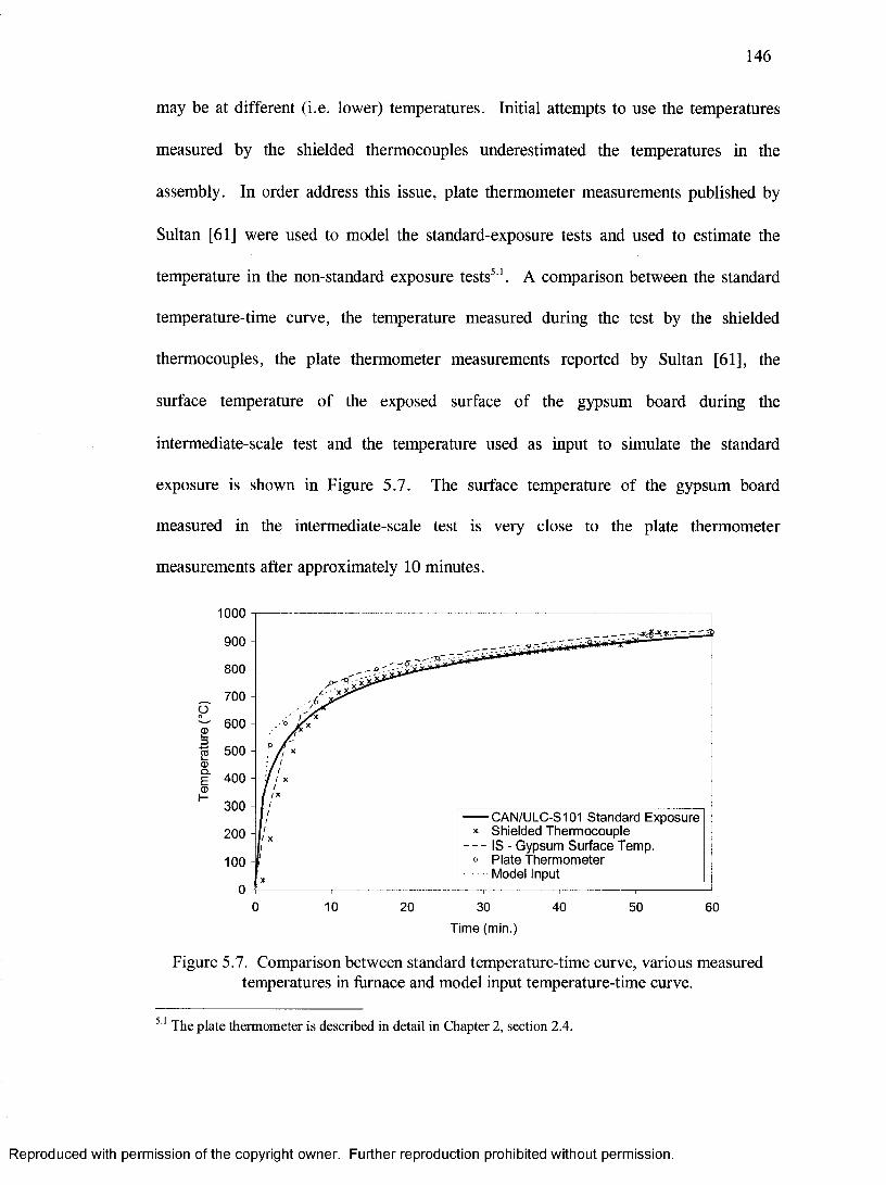
Figure 5.7. Comparison between standard temperature-time curve, various measured
temperatures in furnace and model input temperature-time curve 146
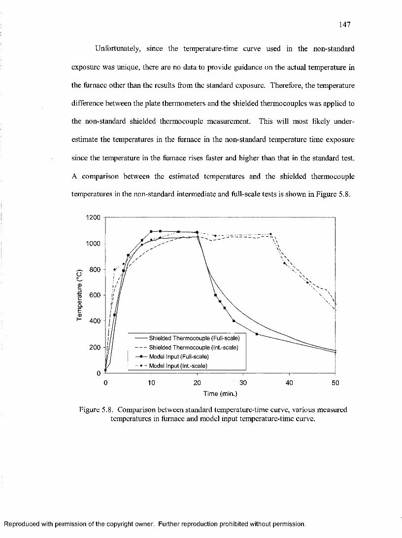
Figure 5.8. Comparison between standard temperature-time curve, various measured
temperatures in furnace and model input temperature-time curve 147
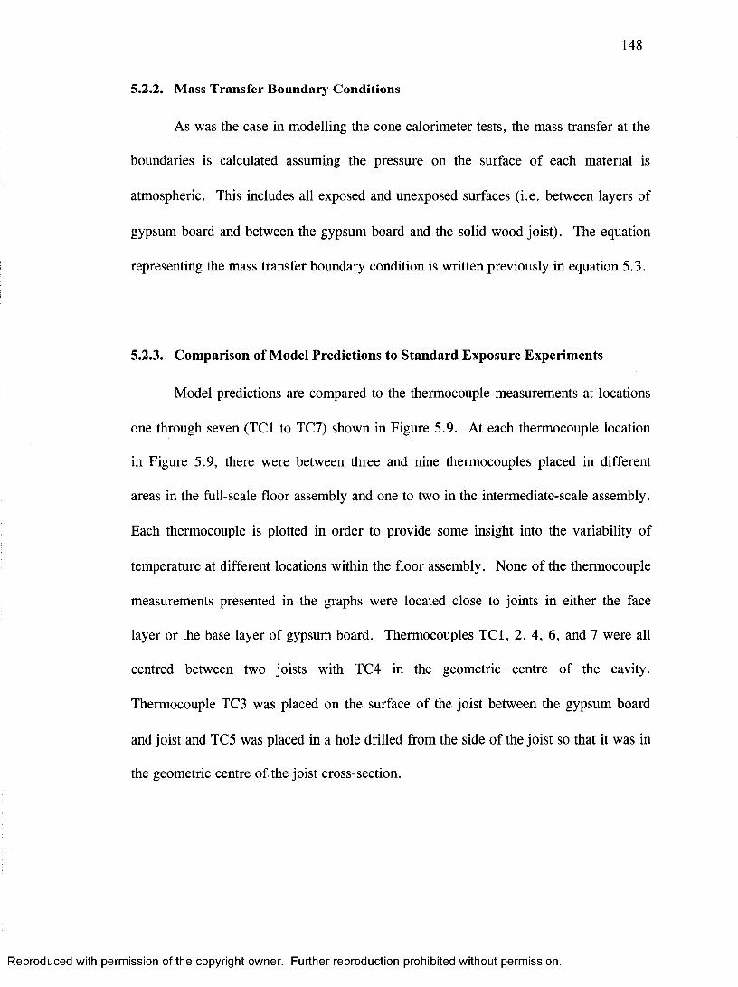
Figure 5.9. Thermocouple locations used in comparison between model predictions and
experiment 149
Figure 5.10. Comparison between temperatures measured at TCI and model predictions.
150
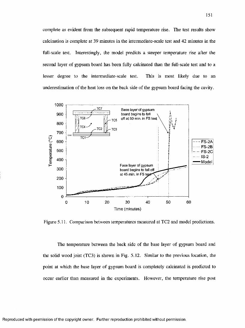
Figure 5.11. Comparison between temperatures measured at TC2 and model predictions.
151
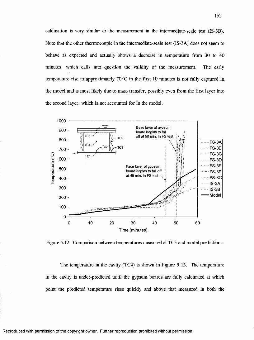
Figure 5.12. Comparison between temperatures measured at TC3 and model predictions.
152
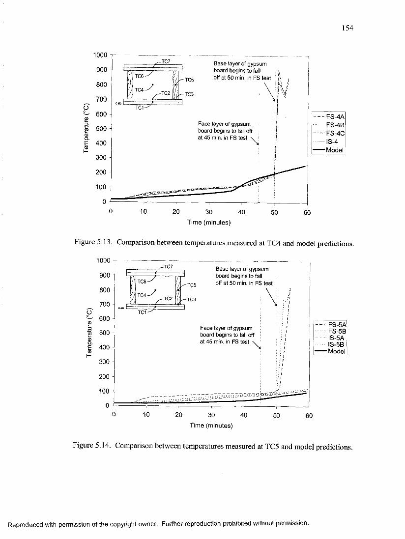
Figure 5.13. Comparison between temperatures measured at TC4 and model predictions.
154
Figure 5.14. Comparison between temperatures measured at TC5 and model predictions.
154
Figure 5.15. Comparison between temperatures measured at TC6 and model predictions.
155
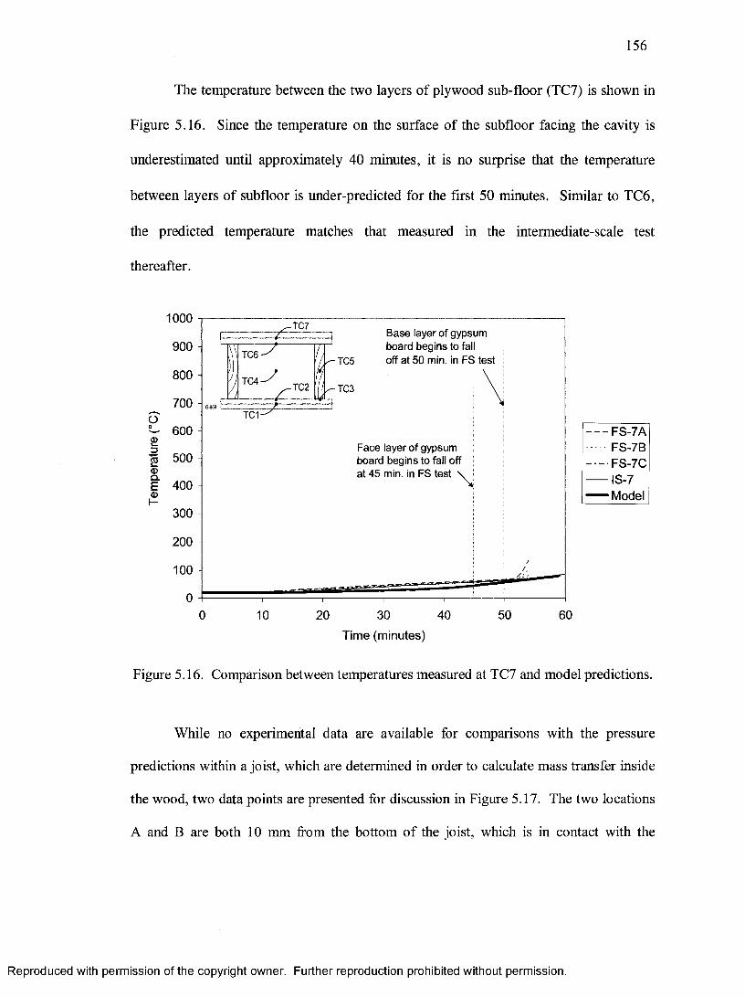
Figure 5.16. Comparison between temperatures measured at TC7 and model predictions.
156
Figure 5.17. Temperature and pressure predictions inside joist with standard exposure
compared to measured temperatures in full-scale test 158
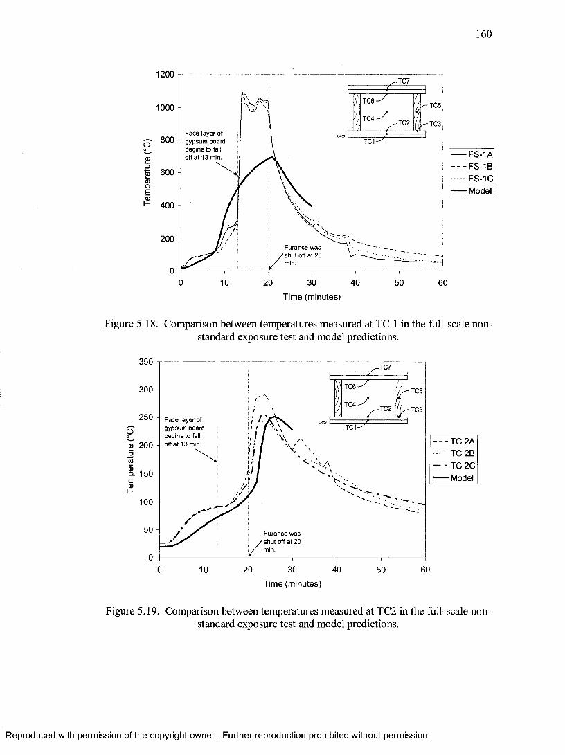
Figure 5.18. Comparison between temperatures measured at TC 1 in the full-scale non
standard exposure test and model predictions 160
Figure 5.19. Comparison between temperatures measured at TC2 in the full-scale non
standard exposure test and model predictions 160
xvi
Reproduced with permission of the copyright owner. Further reproduction prohibited without permission.
Figure 5.20. Temperature and pressure predictions inside joist in foil-scale, non-standard
exposure test 161
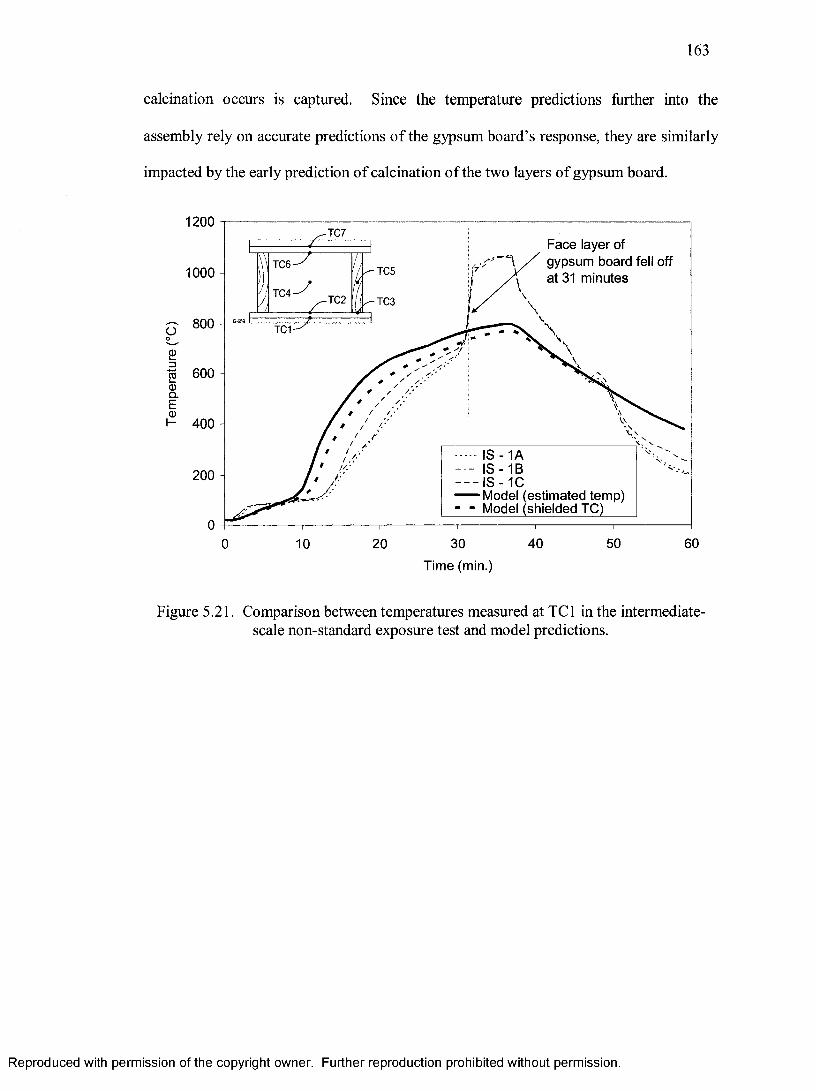
Figure 5.21. Comparison between temperatures measured at TCI in the intermediate-
scale non-standard exposure test and model predictions 163
Figure 5.22. Comparison between temperatures measured at TC3 in the intermediate-
scale non-standard exposure test and model predictions 164
Figure 6.1. Material orientation and finite element mesh used in the simulation 168
Figure 6.2. Gypsum board thermal conductivity as a function of temperature 172
Figure 6.3. Simulation results showing effect of gypsum board thermal conductivity on
the predicted temperature between gypsum board and wood as a function of time. 173
Figure 6.4. Gypsum board specific heat as a function of temperature 174
Figure 6.5. Simulation results showing effect of gypsum board specific heat variation on
the predicted temperature between gypsum board and wood as a function of time. 175
Figure 6.6. Simulation results showing effect of gypsum board density on the predicted
temperature between gypsum board and wood as a function of time 177
Figure 6.7. Simulation results showing effect of gypsum board gypsum content on the
predicted temperature between gypsum board and wood as a function of time 179
Figure 6.8. Simulation results showing effect of gypsum board permeability on the
predicted temperature between gypsum board and wood as a function of time 181
Figure 6.9. Wood thermal conductivity as a function of temperature 183
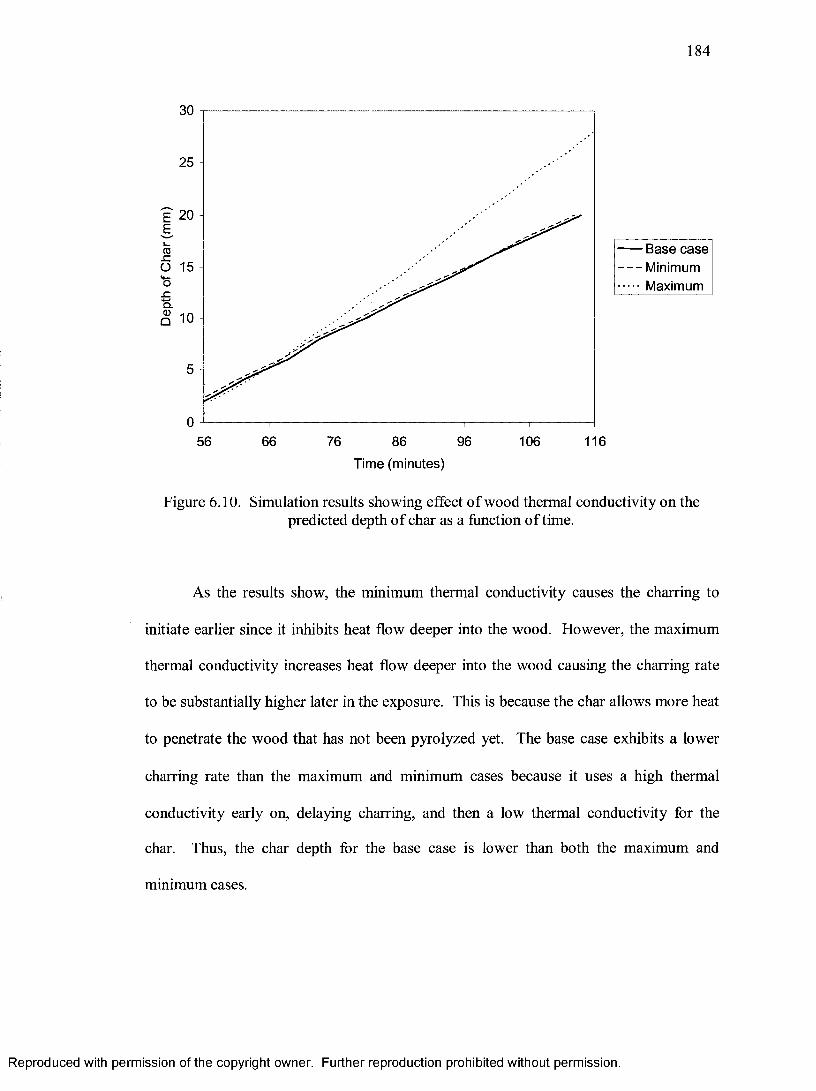
Figure 6.10. Simulation results showing effect of wood thermal conductivity on the
predicted depth of char as a function of time 184
Figure 6.11. Wood specific heat as a function of temperature 185
Figure 6.12. Simulation results showing effect of wood specific heat on the predicted
depth of char as a function of time 186
Figure 6.13. Simulation results showing effect of wood density on the predicted depth of
char as a function of time 187
Figure 6.14. Simulation results showing effect of wood permeability on the predicted
depth of char as a function of time 188
xvii
Reproduced with permission of the copyright owner. Further reproduction prohibited without permission.
Nomenclature
A - pre-exponential constant used in Arrhenius expression, s"1
As - surface area, m2
c - specific heat, J kg"1 K"1
cgas - specific heat of the gas (in cavity of floor assembly), J kg"1 K"1
c(Avg) " average specific heat from ambient temperature to the current temperature, J
kg1 K-1
cACT - specific heat of the active material, J kg-1 K"1
CN-ACT " specific heat of the non-active material, J kg"1 K"1
cACT(Avg) " average specific heat of the active material from ambient temperature to the
current temperature, J kg"1 K"1
c vpp - specific heat of the volatile pyrolysis products, J kg"1 K"1
c vpp(Avg) " average specific heat of volatile pyrolysis products from ambient
temperature to the current temperature, J kg"1 K"1
cw - specific heat of liquid water, J kg"1 K"1
cw(Avg) " average specific heat of liquid water from ambient temperature to the current
temperature, J kg"1 K"1
cwv - specific heat of water vapour, J kg"1 K"1
cwv(Avg) " average specific heat of water vapour from ambient temperature to the
current temperature, J kg"1 K"1
D - permeability, m2
xviii
Reproduced with permission of the copyright owner. Further reproduction prohibited without permission.
Dx - permeability in the x-direction, m2
Dy - permeability in the y-direction, m2
Ea - activation energy used in Arrhenius expression, J mol"1
Egen - rate of energy generated, W
Ejn - rate of energy flowing into the control volume, W
Eout - rate of energy flowing out of the control volume, W
^stored " rate °f change in energy stored, W
Fs2-s - configuration factor between radiating and emitting surfaces
h - specific enthalpy of gas, J kg"1
hAcr " specific enthalpy of the active material, J kg"1
hconv - convective heat transfer coefficient, W m"2 K"1
hVpp " specific enthalpy of volatile pyrolysis products, J kg"1
hw - specific enthalpy of liquid water, J kg"1
h wv - specific enthalpy of water vapour, J kg"1
k - thermal conductivity, W m'K"1
kx - thermal conductivity in the x-direction, W m 'K"1
ky - thermal conductivity in the y-direction, W m"'K"'
kDi - pre-exponential constant used in equation 2.5, m2
ko2 - exponential constant used in equation 2.5, (no units)
LR - heat of reaction, J kg"1
LY - latent heat of vaporization of water, J kg"1
M - moisture content of wood, %
xix
Reproduced with permission of the copyright owner. Further reproduction prohibited without permission.
Meff - effective molecular weight of the gas, kg mol"'
Mw - molecular weight of water, kg mol"1
m - mass, kg
Mgen - rate at which mass of water vapour or volatile pyrolysis products are
generated, kg s"1
Min - rate at which mass enters the control volume, kg s"1
Mout - rate at which mass leaves the control volume, kg s"1
Mstored - rate at which mass is stored in the control volume, kg s"1
mx - mass flow of gases in the x-direction, kg s"1
my - mass flow of gases in the y-direction, kg s"1
m" - mass flow per unit area, kg m"2 s"1
rh" - mass flow per unit area in the x-direction, kg m"2 s"1
m" - mass flow per unit area in the y-direction, kg m"2 s"1
ihypp - mass flow per unit area of volatile pyrolysis products, kg m"2 s"1
ih'^y - mass flow per unit area of water vapour, kg m"2 s"1
m"' - mass per unit volume, kg m"3
m'"tT - mass per unit volume of active material, kg m"3
mow - mass of dry wood per unit volume, kg m"3
m"'K, - mass of wood per unit volume at a specific moisture content, kg m"3
mN-ACT " mass Per unit volume of the non-active material, kg m"3
m"w - mass of solid wood (with no voids or pores) per unit volume, kg m"3
xx
Reproduced with permission of the copyright owner. Further reproduction prohibited without permission.
2 m'w - mass of liquid water per unit volume of material, kg m"
m'" - mass per unit volume at time t, kg m"
m'"pl< - mass per unit volume of volatile pyrolysis products, kg m"3
m* v - mass per unit volume of water vapour, kg m"3
m'" - original mass per unit volume, kg trf
3 1 rn"'( T - rate of change mass of active material per unit volume, kg m" s"
™gen " rate °f at which mass of gases are generated per unit volume, kg rrf3 s"1
iii™ - rate of change mass of liquid water per unit volume, kg m"3 s"1
n - number of moles of gas
P - pressure, Pa
PEVP - equilibrium vapour pressure, Pa
Pwv - partial pressure of water vapour, Pa
Ps - pressure at surface of material, Pa
Pr - ambient pressure, Pa
qx - heat flow in the x-direction, W
qy - heat flow in the y-direction, W
q" - heat flux, W m"2
^cone " ^at flux produce by cone calorimeter, W m"
q" - heat flux in the x-direction, W m"2
q" - heat flux in the y-direction, W m"2
q"omi - heat flux due to conduction, W m"2
xxi
Reproduced with permission of the copyright owner. Further reproduction prohibited without permission.
q"onv - heat flux due to advection, W m"2
q'g'vAp - rate of heat generation per unit volume due to evaporation of water, W m"3
q™n - ra te o f hea t genera t ion per un i t vo lume, W m" 3
q,"R - rate of heat generation per unit volume due to chemical reactions, W m"3
R - gas constant, 8.314 J K"1 mol-1
S - specific gravity
t - time, s
ts - time-step duration, s
T - temperature, K
Tgas - gas (in cavity of floor assembly) temperature, K
TF - effective furnace temperature, K
Ts - temperature at surface, K
To - initial temperature, K
Tro - ambient temperature of surroundings, K
V - Volume, m3
x - dimension in the x-direction, m
y - dimension in the y-direction, m
z - dimension in the z-direction, m
Greek Letters
s - emissivity
seff - effective emissivity
2 1 v - kinematic viscosity, m s"
xxii
Reproduced with permission of the copyright owner. Further reproduction prohibited without permission.
Pgas - gas (in cavity of floor assembly) density, kg m"3
pw - density of liquid water, kg m"3
(p - porosity, m3 m"3
a - Stefan-Boltzmann constant, 5.67 x 10"8 W m"2 K"4
Note: Symbols in bold indicate vectors.
xxiii
Reproduced with permission of the copyright owner. Further reproduction prohibited without permission.
1
1. Introduction
The fire safe design of buildings in Canada has traditionally been met by
following a prescriptive building code. With the introduction of an objective-based
Canadian code in 2005 [1], it is now possible to construct a building that deviates from
the prescriptive code but meets its objectives, provided that the alternative design is as
safe as the prescriptive solution. It is necessary to be able to determine the risk to life and
property of prescriptive and alternative designs in order to make the comparison. In
order to achieve this, a risk assessment model called CURisk has been developed at
Carleton University [2] for four-storey, wood-frame buildings. A number of submodels
are needed to calculate the overall risk due to fire. For example, submodels are used to
characterize fire growth, smoke movement and occupant response and movement.
Another important submodel needed characterizes the response of building assemblies to
fire, which is the focus of this study. This submodel will provide input to the risk model
that may affect fire spread between compartments as well as smoke movement and,
potentially, occupant movement.
Building regulations require that key building assemblies exhibit sufficient fire
resistance to allow time for occupants to escape and minimize property losses. The intent
is to compartmentalize the structure to prevent the spread of fire and smoke, and to
ensure structural adequacy to prevent or delay collapse. The fire resistance of building
assemblies has traditionally been assessed by subjecting a replicate of the assembly to the
standard fire-resistance test, (CAN/ULC S101 in Canada [3], ASTM El 19 in the U.S.A
[4] and ISO 834 in many other countries [5]).
Reproduced with permission of the copyright owner. Further reproduction prohibited without permission.
2
Unfortunately, the standard fire-resistance test used to evaluate assemblies for
code compliance does not provide the necessary information to predict the response of an
assembly subjected to alternative fire exposures resulting from different fire scenarios.
While alternative testing could provide the information needed, the expense and number
of tests required cause it to be uneconomical. Therefore, the only practical solution is
computer modelling.
In order to reduce the need for full-scale testing and to gain a better understanding
of the parameters affecting the fire-resistance of light-frame wood assemblies, a number
of computer models have been developed in recent years [6-9]. The main challenge in
predicting the response of assemblies exposed to fire is modelling the response of
individual materials. There continues to be a paucity of robust material property data for
common building materials at elevated temperatures. Therefore, modelling efforts
continue to make simplifications for the behaviour of materials at elevated temperatures.
An example of one of these simplifications is treating pyrolysis of wood and calcination
of gypsum board as occurring over fixed temperature ranges. This is accomplished by
adding the energy associated with the reactions to the apparent specific heat of the
materials within the temperature range the reactions are assumed to occur. Another
simplification is the calibration of material properties, specifically thermal conductivity,
in order to account for the contribution of mass transfer of water vapour and pyrolysis
products to heat transfer in a material. These simplifications work well in the standard
fire-resistance test where the exposure temperature increases monotonically at a specified
rate. However, when the rate of heating differs from that in a standard test, the
temperature range in which these reactions occur also changes. The fire exposure in
Reproduced with permission of the copyright owner. Further reproduction prohibited without permission.
3
different fire scenarios can differ appreciably from the standard fire-resistance test in the
rate of temperature rise, the peak temperature reached, and the occurrence of a decay
phase after the fuel has been consumed.
Wood buildings up to four storeys in height are permitted to be built in Canada.
Wood buildings can be built using either dimensioned lumber which is referred to as
light-frame construction or using large timber sections which is referred to as heavy
timber construction. Light-frame wood assemblies that require a fire-resistance rating are
typically comprised of one or more layers of gypsum board fastened to the structural
wood members to protect them from the risk of fire exposure. Heavy timber assemblies
often are able to meet the fire-resistance requirements with no additional protection since
the large timbers slowly and predictably loose structural capacity when subjected to fire.
This study is focused on light-frame wood floor assemblies protected by fire-rated
gypsum board. A number of gypsum board products exist including regular gypsum
board, fire-rated type X gypsum board which meets a minimum level of performance in a
standard fire-resistance test, and fire-rated type C gypsum board which is strictly a
proprietary product and is utilized through product listings. Gypsum board's excellent
fire resistance derives from the fact that the core of the board is primarily gypsum, which
contains 21 percent by mass chemically bound water [6], and a vast amount of energy is
required to release and evaporate this chemically bound water. When an engineer or
architect is designing a light-frame wood assembly that requires a fire-resistance rating,
the designer can specify a wall or floor assembly's details based on a proprietary listing
that meets the required fire-resistance rating, or choose an assembly from the National
Building Code (NBC) using one of two methods available based on the building type. If
Reproduced with permission of the copyright owner. Further reproduction prohibited without permission.
4
the building fits within the definition of "housing and small buildings", then the designer
can choose an assembly from the generic tables provided. If the building is larger or
contains an occupancy that does not allow the use of the generic tables, then an assembly
can be designed using the component additive method (CAM) where each component of
the assembly is assigned a contribution to the fire-resistance of the overall assembly. The
design objective for all of these methods is to calculate the fire-resistance rating which
would otherwise be obtained from a standard fire-resistance test. However, these design
methods do not provide guidance on predicting the performance when assemblies are
subjected to design (realistic) fires.
1.1. Objective and Scope of Study
The objective of this study is to develop a model to simulate the thermal response
of a light-frame wood assembly protected by gypsum board regardless of the heating rate
and initial conditions (such as moisture content of the wood). The model is intended to
simulate the heat and mass transfer within the gypsum board and wood when an assembly
is subjected to any fire condition. In order to evaluate the accuracy of the model, a series
of experiments have been conducted to generate empirical data, which are then compared
with model predictions. The scope of this study has been limited to wood-frame floor
assemblies constructed with solid-sawn wood joists.
Reproduced with permission of the copyright owner. Further reproduction prohibited without permission.
5
1.2. Contribution of this Study
The coupled heat and mass transfer model that has been developed and
implemented to predict the temperature rise throughout the floor assembly when exposed
to fire is the first to include mass transfer in both gypsum board and wood in two-
dimensions. The model more closely simulates the response of both gypsum board and
wood to fire, increasing the accuracy of predictions for a wide range of different fire
exposures that would be expected from different fire scenarios. Improved models for
calcination of gypsum board and pyrolysis of wood more accurately predict the
temperatures at which the reactions take place regardless of the rate of heating. The
information generated on the response of a light-frame wood assembly to fire is needed
for both performance-based design of assemblies to any particular fire and as an input to
CURisk, allowing the risk to life and property for wood buildings to be determined for
optimization of designs by including the response of the structure to fire.
Reproduced with permission of the copyright owner. Further reproduction prohibited without permission.
6
2. Literature Review
In this chapter, the results of a literature review are presented to summarise what
has been accomplished by past researchers in the area of modelling light-frame wood
assemblies exposed to fire. The standard fire-resistance test is reviewed in the following
section. Next, the models that have been developed in the past to predict the response of
light-frame wood assemblies exposed to fire are reviewed. Subsequently, the data
necessary to develop a model to predict the response of gypsum board and wood exposed
to fire are reviewed and summarized. Finally, a review of papers that have investigated
the conditions inside the fire-resistance furnace necessary for modelling the heat transfer
to the specimen is undertaken.
2.1. Standard Fire-Resistance Testing
The standard fire-resistance test is the test method used to evaluate the fire
performance of structural members and assemblies as well as assemblies or components
of assemblies used to limit the spread of fire and smoke. The standard fire-resistance test
used in Canada is CAN/ULC-S101 [3], the United States uses ASTM El 19 [4] and many
other countries adopt directly, or with some modification, the international standard ISO
834 [5], In all three standards, a structural member or assembly is tested by subjecting it
to a standard temperature-time exposure. In the case of a wall assembly, the assembly
forms one wall of the furnace while in the case of a floor assembly, the assembly forms
the top of the furnace. Floor assemblies are then loaded and the temperature inside the
furnace is increased at a prescribed rate. The floor furnace, temperature exposure and
failure criteria are explained below.
Reproduced with permission of the copyright owner. Further reproduction prohibited without permission.
7
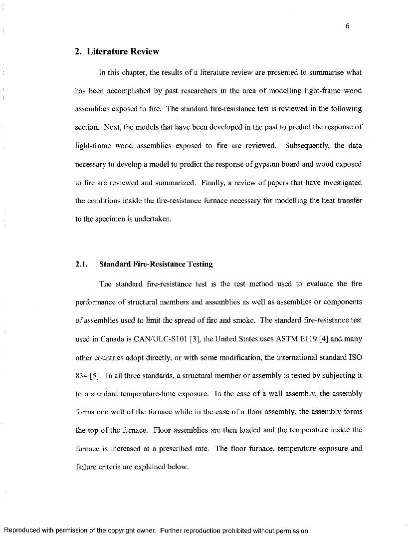
2.1.1. Fire-resistance Floor Furnace and Test Assembly
The floor furnace is made up of a floor and four sides with the top left open in
order to accept the floor/ceiling assembly to be tested as shown in Figure 2.1. A typical
furnace accepts a floor assembly approximately four meters wide by five meters long
which is built within a test frame that can be lowered onto the furnace. The floor furnace
at the National Research Council Canada (NRCC) has a loading frame that connects to
the test frame. This frame applies a load (typically the design load for the assembly)
using a series of hydraulic pistons and pads to distribute the load evenly over the floor
surface. A series of gas burners provide the fuel and air necessary to create the
temperature-time exposure inside the furnace. The temperature is measured using the
average of nine shielded thermocouples.
0!
c
F
SPECIMEN-FLUE
THERMOCOUPLE TUBES
PORTS
GAS BURNERS
Figure 2.1. Typical floor furnace (reproduced from [3]).
Reproduced with permission of the copyright owner. Further reproduction prohibited without permission.
8
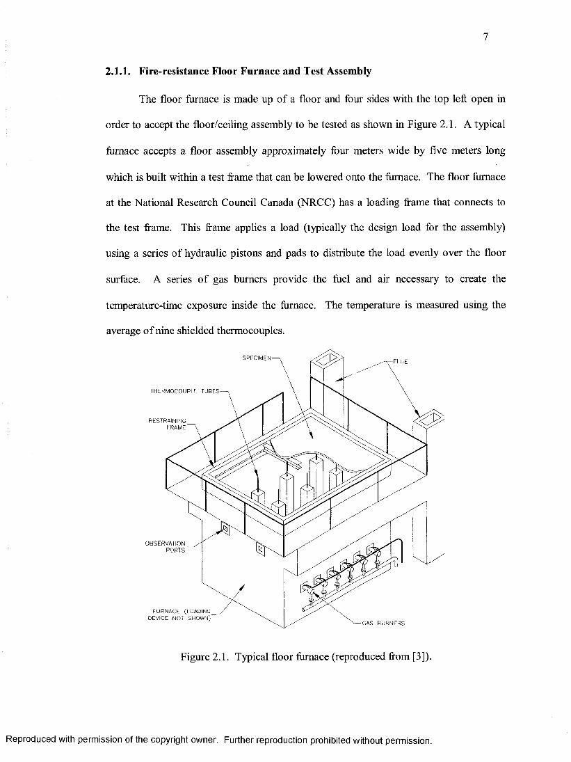
2.1.2. Fire Exposure
The standard temperature-time curve specified in CAN/ULC-S101 [3] is
reproduced in Figure 2.2. The temperature rises very quickly in the beginning reaching
785°C after 20 minutes. The temperature then somewhat levels out reaching 924°C after
one hour and 1007°C after two hours. The temperature inside the furnace is controlled
using shielded thermocouples where the thermocouples are placed inside near the top of
steel pipes, both in order to protect the thermocouple as well as make the furnace easier
to control. The shielded thermocouples prevent the temperature readings from rapidly
changing when the burners in the furnace turn on and off in order to have the furnace
temperature follow the standard temperature-time curve.
1200
1000
800 O o
3 600 2
2L E q; I- 400
200
100 120 80 40 60 20 0
Time (minutes)
Figure 2.2. Temperature exposure as a function of time in the standard fire-resistance test, CAN/ULC SI01 [3].
Reproduced with permission of the copyright owner. Further reproduction prohibited without permission.
9
2.1.3. Failure Criteria and Finish Rating
In the case of light-frame wood floor assemblies, there are three possible failure
criteria that determine the end of the test and the corresponding fire-resistance rating.
Failure has occurred if any of the three criteria are met. First, the floor assembly
experiences structural failure if it can no longer support the applied load. Second, if the
average temperature rise on the unexposed surface of the assembly reaches 140°C above
its initial temperature or if at any location the temperature rise exceeds 180°C, the
assembly is deemed to have experienced insulation failure. Third, the floor assembly is
judged to have experienced integrity failure if the assembly allows the passage of hot
gases or flames hot enough to ignite a cotton pad. The time from the start of the test until
failure is the fire-resistance rating of the assembly rounded to the nearest minute.
The finish rating of the assembly is the time at which a thermocouple placed
between the gypsum board protection and the wood joist reaches the same criterion as for
thermal failure of the assembly (an average temperature rise of 140°C or an individual
temperature rise of 180°C) [10].
Reproduced with permission of the copyright owner. Further reproduction prohibited without permission.
10
2.2. Previously Developed Thermal Models for Light-frame Construction
A number of researchers have investigated heat transfer through light-frame
assemblies (protected by gypsum board) when exposed to fire. Thomas [9] has modelled
the heat transfer from fire through floors using a commercially available finite element
program. Heat transfer through walls exposed to fire has been modelled by Thomas [9],
Takeda and Mehaffey [6, 7, 11], Konig and Walleij [12], Clancy [8, 13-16], Collier [17],
Alfawakhiri [18, 19], Hurst and Ahmed [20], and Gammon [21], Manzello et al. [22]
developed a model to predict one-dimensional heat and mass transfer through a gypsum
board protected wall assembly neglecting the contribution of the studs. Fredlund [23, 24]
has developed a model to determine one-dimensional heat and mass transfer through
wood. A finite element model developed by Sterner and Wickstrom [25] models the
thermal response of structural members exposed to fire. A summary of the work by each
of these authors is given below.
2.2.1. Thomas [9]
Thomas at the University of Canterbury, New Zealand modelled both walls and
floors exposed to the standard fire-resistance temperature-time curve using the finite
element program TASEF [25]. Floors were also modelled using ABAQUS, since TASEF
was not suitable for modelling radiation around re-entrant corners. All material
properties used in the simulations were taken from the literature. The material properties
were assumed correct and the convective heat transfer coefficients were modified in order
to obtain good agreement with experimental results. The mass transfer of moisture was
not modelled, however, in an effort to compensate for this omission, the thermal
Reproduced with permission of the copyright owner. Further reproduction prohibited without permission.
conductivity of wood was doubled between 60°C and 110°C. The model produced
temperature predictions that were closer to the experimental measurements when using
the increased thermal conductivity. The author claimed that the net effect of moisture
movement is insignificant when temperatures surpass 120°C. The geometry was set up
to allow a gap to form between the gypsum and the studs/joists as the author believed the
gap formed due to shrinkage of the wood and subsequent char. The gap was assumed to
be constant at 1 mm for the entire test, since this gave good agreement with the
experiments.
The predictions of the wall model were in good agreement with experimental
data, however, the model was found to overestimate temperatures for fast, hot fires. The
model was also found to under-predict temperatures in the stud when the lining material
was thin. The time to onset of charring was under-predicted in all cases, while insulation
failure was not consistently conservative (i.e. underestimated).
The floor models were found to give good agreement with the experiment. When
the TASEF and ABAQUS models were compared for the solid wood joists configuration,
the results were almost identical. This was expected since the material property data and
boundary conditions used in the simulations were identical.
2.2.2. Takeda and Mehaffey [6, 7,11]
A model called WALL2D (and more recently WALL2DN) has been developed at
FPInnovations - Forintek Division (formerly Forintek Canada Corp). WALL2D is a
two-dimensional computer model which predicts heat transfer through non-insulated
wood-stud walls protected by gypsum board. The model solves the governing equation
Reproduced with permission of the copyright owner. Further reproduction prohibited without permission.
using explicit finite-difference techniques. Material property data have been taken from
tests performed on Canadian gypsum board and wood at the NRCC. In order to ensure
that the large peak in specific heat due to calcination of gypsum board was captured, an
enthalpy formulation was used for heat transfer. The newest additions to the model
WALL2DN include the modelling of four different insulation types in the wall cavity and
modelling shrinkage of gypsum board in order to simulate the opening of joints between
boards. The modelling of insulation includes shrinkage away from the fire exposed
gypsum board at elevated temperatures as well as changes in thermal conductivity with
temperature. The shrinkage of gypsum board was modelled using the temperature of the
unexposed surface of the gypsum board. Once the joints begin to open, the model allows
for convection but not radiation on the exposed stud and the exposed ends of the gypsum
boards. Gypsum board pull-off from the wall assembly was assumed to occur when the
shrinkage of the gypsum board results in the edge fasteners no longer holding the gypsum
board. Once the criteria are met for gypsum board fall-off, the cavity temperatures are
set to the furnace temperature. The grid size used varies from 1.59 mm (1/16 in.) on the
surface of the wood and gypsum to 3.18 mm (1/8 in.) for the interior of the materials.
The time-step used in the analysis was 1 second.
Model predictions for heat transfer through the gypsum board, across the cavity
(with and without insulation), and through the gypsum board on the ambient side were in
good agreement with experimental data. The accuracy in modelling heat transfer through
the wood studs was less satisfactory. The temperature was overestimated on the fire side
of the stud and on the unexposed side of the stud the temperature was underestimated
compared to experimental data. This was most likely due to moisture movement within
Reproduced with permission of the copyright owner. Further reproduction prohibited without permission.
the wood stud, which was not taken into account in either version of WALL2D. The
model was written in such a way that it is not easy to make modifications to geometry
and the model was not capable of modelling the decay phase of a fire.
2.2.3. Konig and Walleij [12]
A two-dimensional finite element thermal model called TEMPCALC has been
developed at the Swedish Institute for Wood Technology Research. The purpose of the
model was to determine the progress of the char-line and the temperature field in an
assembly. The model has been used for wood-stud walls, however there seems to be no
reason it could not be used for floors with some simple modification. The effect of mass
transfer was not accounted for. The model was built in stages, with testing after each
stage before adding another component to the assembly. The lining on the ambient side
of the assembly was neglected in the model, however, no details were provided on the
boundary condition used on the unexposed surface. Material properties were taken from
the literature with some modification through calibration of the model results to
measurements of the temperature taken in standard fire-resistance tests. Unfortunately,
detailed information on the model, including verification of the model predictions, was
not described in this report. Comparisons between model predictions and experiment
results are made only for the char depth as a function of time. The calculated values
seem very close to the test results in some cases and less so for others.
Reproduced with permission of the copyright owner. Further reproduction prohibited without permission.
14
2.2.4. Clancy [8,13-16]
A thermal model called ADIDRAS was developed at the Victoria University of
Technology, Australia, for modelling heat transfer in walls. The model is a two-
dimensional numerical algorithm that uses an alternating direction implicit finite
difference method of analysis. The methodology used in the model is similar to previous
heat transfer models such as that produced by Takeda and Mehaffey [7]. In this model,
material property data have been taken from the literature. Advances to the modelling of
heat transfer within the wall include a method to predict the radiative heat transfer in
cavities which have re-entrant corners. The model also accounted for suspected
shrinkage gaps that develop between the wood and gypsum as the wood dries and
shrinks. This causes a decrease in the heat transfer to the stud after shrinkage has taken
place, resulting in lower temperatures on the exposed side of the stud. By using a 1 mm
gap between the stud and gypsum board, better agreement with experimental
temperatures were found between the exposed gypsum board and the stud. Clancy also
tried to account for increased heat transfer due to moisture movement by increasing the
thermal conductivity by a factor of 10 for wood and gypsum board, for temperatures less
than or equal to the vaporization temperatures. Fall-off of the gypsum board was
assumed to occur when the temperature on the unexposed side of the gypsum board
reached the approximate melting point of the glass fibres in the board (approx. 700°C).
This method seemed to over-estimate the temperature rise on the edge of the stud
closest to the fire, while underestimating the rise in temperature on the edge of the stud
furthest from the fire. Overall, however, good agreement with experimental values was
found. By taking into account moisture movement, which was considered through
Reproduced with permission of the copyright owner. Further reproduction prohibited without permission.
15
increased thermal conductivity, and the shrinkage gap between the stud and the gypsum,
better agreement with experimental values was obtained for the examples given. Clancy
concludes that in areas within solids where the temperature is below 100°C, moisture
transfer greatly increased heat transfer rates and in areas where the temperature is
between 100°C and 150°C, moisture transfer reduced heat transfer rates. Above 150°C,
moisture was believed not to affect the heat transfer.
2.2.5. Collier [17]
A one-dimensional finite difference model was developed at BRANZ, New
Zealand, which predicts the temperature rises across the cavity section of a structural wall
exposed to both standard and non-standard (realistic) fires.
The model used thermal properties from the literature. Thermal exposure to the
wall was modelled using exposure conditions measured during experiments. Attempts to
account for ablation of the gypsum board and combustion of the wood studs and paper
products within the model were not entirely successful and no attempt was made to
model or account for the energy movement associated with mass transfer.
Verification of the model was completed by comparing the predictions to the
results of four small-scale fire tests. The time to onset of charring was underestimated for
all tests and the decay phase was not well predicted. The model did not provide
sufficient information to model the structural response since the temperatures calculated
are in one dimension.
Reproduced with permission of the copyright owner. Further reproduction prohibited without permission.
16
2.2.6. Alfawakhiri [18,19]
A computer model called TRACE was developed at Carleton University, Canada,
to predict the heat transfer through an insulated light-frame steel assembly. Heat transfer
was determined using a one-dimensional finite difference analysis. The model
considered radiation and convection heat transfer to the exposed gypsum board surface,
conduction through the gypsum board, conduction through the insulation, conduction
through the gypsum board on the unexposed side, and radiation and convection from the
unexposed gypsum board surface to the ambient surroundings. The model ignored the
heat transfer through the metal studs, as well as moisture movement in the gypsum board
and the opening of joints due to gypsum board shrinkage. Material properties were
calibrated using full-scale test data. The model predictions compared well with the
experimental data. Predictions of the cavity temperatures, however, were not as accurate.
2.2.7. Hurst and Ahmed [20]
A computer model developed by the Portland Cement Association was used to
analyze the thermal response of wood-framed gypsum board assemblies subjected to the
ASTM El 19 standard fire exposure. The model predicts the coupled heat and mass
transfer through gypsum board by considering the dehydration process and the effect it
has on pore size and the mass transport mechanism. The material property data used in
the analysis were not reported in the paper. The solution of the equations for
conservation of mass, momentum, and energy were obtained using a fully implicit finite
difference scheme.
Reproduced with permission of the copyright owner. Further reproduction prohibited without permission.
17
The predictions of the model were found to be in good agreement with previous
experimental tests, however, the model did not consider the effects of wall studs, and
therefore provided no insight into temperature within a stud. The authors proposed that
hot gases being forced through cracks and/or open joints under positive pressure have a
significant effect on the fire performance.
2.2.8. Gammon [21]
A finite element model called FIRES-T3 developed at the University of
California, Berkeley, was used to model the heat transfer and structural response of light-
frame wood-stud walls. The finite element method was chosen for the analysis due to the
ease in changing the geometry when using this method. The heat transfer analysis
neglected the effects of moisture movement and the convection heat transfer in the wall
cavities. Insulation in wall cavities was not modelled. The material properties were
taken from the literature. The author discussed a method to carry out a probability and
reliability analysis, but cites lack of data for not being able to complete the analysis.
The results of the simulations were, for the most part, in agreement with the
results of published ASTM E-l 19 wall tests. Changes in the thickness of the wall linings
did not always lead to changes in endurance time that were of the same magnitude as
those reported in the literature. Simulations of a wood slab exposed to fire on one side
were performed to predict the rate of char advance through wood with excellent
agreement with published data. The model included the reduction in thickness of the
gypsum board due to ablation, which is the slow erosion of the exposed surface at high
temperatures. The model predictions were found to be very sensitive to the temperature
Reproduced with permission of the copyright owner. Further reproduction prohibited without permission.
used for the onset of ablation and there was some uncertainty as to what temperature
should be used.
2.2.9. Manzello et al. [22]
A two-dimensional model was developed at the National Institute of Standards
and Technology in the United States to predict the response of gypsum board to real fires.
The governing equations used in the model consist of gas-phase conservation equations,
liquid-phase conservation equations, momentum conservation (according to Darcy's
Law) and the energy conservation equation. The cavity of the wall was modelled using a
lumped thermal capacity approach. The analysis was limited to the gypsum board layers
and the space between the layers with no consideration for the studs. The paper does not
give any insight into the material properties used in the simulation. Comparisons were
made between experiments that were completed on non-load bearing steel stud walls
exposed to a real fire, which was intended to represent an office occupancy. The model
accurately predicted the point at which calcination is complete. Following calcination,
the temperature increased rapidly on the backside of the gypsum board, and the model
was found to under-predict this temperature rise. It was proposed that the under-
prediction was due to physical changes in the gypsum board (cracks and opening of
joints), which allowed heat into the assembly earlier than predicted by the thermal model.
Reproduced with permission of the copyright owner. Further reproduction prohibited without permission.
19
2.2.10. Fredlund [23,24]
A computer model called WOOD1 was developed at Lund University, Sweden, to
predict one-dimensional heat and mass transfer in wood exposed to fire. The model
accounted for the thickness, density, and moisture content of the wood. The model
predicted the temperature profile, density distribution, and moisture profile in the wood.
Heat transfer is assumed to occur by conduction as well as by advection due to the
flow of volatile pyrolysis products and water vapour through the pore system of the
wood. The equations of heat and mass transfer are solved using the finite element
method. Mass transfer is assumed to be affected primarily by pressure-driven flow, and
therefore, diffusion is ignored. The model alters the geometry of the structure as the
surface of the material is oxidized. All material property data used was taken from the
literature.
Fredlund found that the distribution of temperature in the experiments were
predicted very well for both moist and dry material. The model produced satisfactory
predictions of mean pressure in the pores, but it was found to be difficult to measure
pressure near the char due to cracks that form in the char layer.
WOOD1 models only one dimensional heat and mass transfer in wood. In order
to model heat and mass transfer in an assembly, a two dimensional model would be
needed along with consideration for the other components of a floor assembly. In order
for the model to capture the steep pressure gradients, it was found that short time-step
increments and small elements (e.g. 1 sec., 1 mm) were needed.
Reproduced with permission of the copyright owner. Further reproduction prohibited without permission.
20
2.2.11. Sterner and Wickstrom [25]
A model called TASEF was developed at the Swedish National Testing Institute.
TASEF is a two-dimensional finite element model developed to calculate the temperature
in structures exposed to fire. The model includes an input data generator in order to
formulate the input file for the model.
TASEF employs an explicit forward difference time integration scheme. The
time-step is constantly determined based on a percentage of the maximum time step
calculated. The thermal conductivities of materials are specified at a number of
temperature levels and are assumed to vary linearly between points. The heat capacity is
indirectly input by the specific volumetric enthalpy. The radiation within voids of the
structure is calculated using view factors calculated using Hottel's crossed-string method.
The model is limited to materials which are isotropic in the two orthogonal directions
considered in the analysis.
Reports give examples where TASEF has been applied; however, all examples
given are for concrete and/or steel. The authors report good results have been found for
predicting the temperature in steel and to a lesser extent concrete when exposed to fire.
The less robust material property data for concrete, compared to steel, and the fact that
the model fails to account for mass transfer are cited as possible reasons for the
difference in accuracy between steel and concrete. The effects due to water vapour
migration and degradation of material cannot be modelled with TASEF. Therefore, this
model cannot account for either ablation of the gypsum board or the moisture transfer in
either the wood joists or gypsum.
Reproduced with permission of the copyright owner. Further reproduction prohibited without permission.
21
2.2.12. Summary of Available Models
The literature review uncovered nine computer models developed to predict the
response of light-frame assemblies protected by gypsum board exposed to fire and one to
predict the behaviour of wood exposed directly to fire. In summary, the following
observations have been made:
> Mass transfer has not been included explicitly in modelling light-frame wood
assemblies.
> Two papers have modelled the heat and mass transfer in gypsum board alone to
predict the response of assemblies with steel studs.
> Commercially available finite element models are unable to model mass transfer
and chemical reactions such as pyrolysis of wood or calcination of gypsum board.
None of the specially developed computer programs have been made available to
the public.
> Most authors have relied on material property data that has been published in the
literature even though there is a significant variation in reported values,
particularly for gypsum board.
> Most models are unable to model the decay phase of a fire since the material
properties are defined as a function of temperature and, therefore, chemical and
physical changes to the material are reversed as the material cools.
Reproduced with permission of the copyright owner. Further reproduction prohibited without permission.
22
2.3. Review of Material Properties
This section reviews the literature on the response of gypsum board and wood to
elevated temperatures associated with fire and the material properties needed in order to
model the heat and mass transfer in both materials.
2.3.1. Gypsum Board
Gypsum board is the generic name for a group of panel products consisting of a
non-combustible core and a paper surface on each face. The core consists primarily of
gypsum. Gypsum rock is mined or quarried, crushed, ground into a fine powder and then
• 9 1 •
heated to 175°C, driving off three quarters of the chemically combined water. This
leaves calcium sulphate hemihydrate in powder form. This powder (plaster of Paris) is
then mixed with water, soap foam and additives to form a slurry, which is fed between
continuous layers of paper on a board machine. As the board moves down a conveyer
line, the calcium sulphate rehydrates and the gypsum crystals re-form into their original
rock state (calcium sulphate dihydrate). The paper subsequently becomes chemically and
mechanically bonded to the gypsum core. The board is then cut to length and conveyed
through dryers to reduce the free moisture content. It should be noted, however, that a
small amount of free water, approximately 0.5 percent [26], will remain over time in the
board as a result of normal levels of humidity in the air.
21 Gypsum board manufactures are increasingly relying on "synthetic" gypsum as an alternative to natural gypsum. "Synthetic" gypsum is a by-product of manufacturing processes, primarily the manufacturing of titanium dioxide used in paint and desulphurization of flue gases in fossil-fuelled power plants using calcium carbonate. "Synthetic" and natural gypsum have identical chemical compositions. In the USA "synthetic" gypsum currently makes up approximately seven percent of the industry's total calcined gypsum. Traditionally, most plants that incorporated "synthetic" gypsum into their board products relied on a mixture of synthetic and natural core, however, modern plants can manufacture gypsum board without using any natural gypsum.
Reproduced with permission of the copyright owner. Further reproduction prohibited without permission.
23
There are three types of gypsum board available in Canada with respect to fire
performance: regular board, type X board and type C board. Regular gypsum board is
most commonly used in low-rise residential construction (e.g. single-family houses)
where there are no requirements to exhibit a minimum level of structural fire
performance. The board contains no reinforcing other than the external paper. The fire
performance of type X board is specified in ASTM C1396-06a [27], which states that
type X gypsum wallboard "provides not less than 1 hour fire-resistance rating for boards
5/8 in. (15.9 mm) thick or % hour fire-resistance rating for boards lA in. (12.7 mm) thick,
applied parallel with and on each side of load bearing 2x4 wood studs spaced 16 in.
(406 mm) on centre" and tested in accordance with Test Method E 119 [4] (similar to
CAN/ULC-S101 [3]). Fire-rated gypsum board is reinforced with glass fibres in order to
reduce cracking due to shrinkage and contains vermiculite or other materials that expand
when heated to offset the shrinkage of gypsum at high temperatures. Type C board is a
proprietary product that typically exceeds the requirements of type X and its performance
is documented through product listings with organizations such as Underwriters
Laboratories of Canada.
The excellent fire resistance of gypsum board derives from the fact that the core
of the board is primarily gypsum, which is a crystalline mineral that contains
approximately 21 percent by mass chemically bound water. The release of this water is a
two step-process called calcination. The first reaction converts the calcium sulphate
dihydrate (gypsum) to calcium sulphate hemihydrate (plaster of Paris):
CaSQ4 • 2H20 heat >CaS04 iH20 + |H20 (Eq. 2.1)
Reproduced with permission of the copyright owner. Further reproduction prohibited without permission.
24
The second step is the conversion of calcium sulphate hemihydrate to calcium sulphate
anhydrate:
CaS04 -^H20 heat >CaS04 +|h20 (Eq. 2.2)
Both reactions are endothermic and produce liquid water. In addition to the energy
required in this two-step process, a large amount of additional energy is required to
evaporate the water.
A change in the molecular structure of calcium sulphate from a soluble crystal to
an insoluble one was found to occur just above 400°C in Differential Scanning
Calorimetery (DSC) tests [28], where the reaction is slightly exothermic.
Another reaction takes place at temperatures above 600°C, as indicated by
significant mass loss shown in thermal gravimetric analyses (TGA) [29] and DSC tests
[30]. This reaction is the decarbonation of calcium carbonate and produces calcium
oxide (quicklime) and carbon dioxide.
CaC03 heat ) CaO + C02 (Eq. 2.3)
A large variation exists among gypsum board manufacturers and products in the calcium
carbonate content, as this is dependent on the source of gypsum. As with all chemical
reactions, the rates of calcination and carbonation reactions in gypsum board are
dependent on temperature. Therefore, the actual temperature range over which the
reactions occur is a function of the rate of heating.
Reproduced with permission of the copyright owner. Further reproduction prohibited without permission.
25
2.3.1.1. Gypsum Board Thermal Conductivity
Many things affect the effective thermal conductivity of gypsum board, including
moisture movement and the opening of fissures and cracks in the gypsum as it is heated.
All thermal conductivity measurements that have been completed to determine the values
quoted below have been carried out using steady-state conditions. Since the
measurements were carried out under steady-state conditions, moisture movement is not
included. If the thermal conductivity were to include the effects of moisture movement,
it is believed the values would increase from their current estimations. Clancy [14] has
gone so far as to increase the thermal conductivity by a factor of ten for temperatures less
than or equal to the vaporization temperature in an attempt to account for moisture
movement.
The opening of fissures and cracks in the gypsum may increase the effective
thermal conductivity at higher temperatures since radiation heat transfer across the cracks
and fissures becomes greater than conduction heat transfer through the gypsum board.
Depending on the testing method the opening of these cracks and fissures may or may not
occur. For example, in Takeda and Mehaffey [7], the test setup consisted of a heavy
weight on top of the gypsum, which would reduce the chance of fissures opening up. The
change in thermal conductivity with increasing temperature reported by the studies below
can be seen in Figure 2.3.
Reproduced with permission of the copyright owner. Further reproduction prohibited without permission.
26
0.8
0.7 -
2~ 0.6 -E
Takeda and Mehaffey [7] Benichou et al. [31] Sultan [19] Wakili et al. [30]
Figure 2.4. Specific heat of gypsum board as a function of temperature [31].
Interestingly, Wakili et al. [30] found that the temperature at which calcination
begins and the degree to which the two reactions of calcination (shown by two
overlapping peaks in the DSC data) are separated are dependent on the degree to which
the DSC sample is vented when tested at the same heating rate. This is most likely due to
a reduction in the rate of evaporation of water that is produced during calcination,
assuming the venting does not affect the rate of heating.
The specific heat of gypsum board in the absence of the chemical reactions that
take place in the board is relatively constant. Manzello et al. [28] found the specific heat
of type X gypsum board to be 1.2 kW kg_1K_1 at 50°C and also at 600°C. Between
calcination of the gypsum and the conversion of the calcium sulphate anhydrate from a
soluble to an insoluble state, which begins at approximately 400°C, the specific heat was
found to be 1.1 kW kg_1K_1. Mehaffey et al. [6] found the specific heat of gypsum board
to be 0.95 kW kg_1K_1 up to 200°C.
Reproduced with permission of the copyright owner. Further reproduction prohibited without permission.
30
Harmathy [33] reported specific heats after calcination in the range of 0.81 - 0.83
kW kg^K"1 up to 300°C where there was a brief drop, possibly caused by oxidation of a
small amount of organic matter.
Wakili et al. [30] used a specific heat of 1.0 kW kg^K"1 for gypsum board outside
of the temperature ranges where calcination of gypsum and decarbonation of calcium
carbonate takes place. Although it is not explicitly stated, it seems this value was taken
from DSC tests completed on gypsum board and reported in the paper.
Benichou and Sultan [31] found the specific heat above 300°C to actually drop
below zero (indicating the gypsum sample exhibited signs of a slightly exothermic
reaction) up to 600°C, where there was a slight increase in the apparent specific heat most
likely due to the decarbonation of the calcium carbonate. It is not clear why the apparent
specific heat dropped below zero. One possibility is there may have been some organic
matter in the sample that oxidized causing the release of a small amount of heat enough
to drop the apparent specific heat below zero at that heating rate.
2.3.1.3. Gypsum Board Density
The density of gypsum board has some influence on the gypsum board's ability to
protect an assembly from the high temperatures of fire. Richardson and McPhee [34]
found that a reduction of 5.8 percent in board density results in a 7.5 percent reduction in
the fire endurance of the load-bearing wall assembly. The densities of Canadian gypsum
board products found in the literature are reported in Table 2.1.
Table 2.1. Reported gypsum board densities for Canadian fire-rated gypsum board products.
Reproduced with permission of the copyright owner. Further reproduction prohibited without permission.
31
Authors Nominal Thickness
(mm) Type
Density (kg m"3)
Mehaffey^al. [6] 12.7 type C 732
Mehaffey^al. [6] 15.9 type X 648 12.7 regular 620
Craft et al. [29] 12.7 type C 740
Craft et al. [29] 15.9 type X 690 15.9 type X 720 12.7 regular 612 12.7 type X 811 12.7 type X 769
Thomas et al. [35] 12.7 type X 759
Thomas et al. [35] 15.9 type X 750 15.9 type X 730 15.9 typeX 701 15.9 type X 687
Harmathy [33] N/A "fire-rated" 678
Benichou and Sultan [31]
Both 12.7mm and 15.9 mm
type X 654-733 Benichou and Sultan [31]
12.7 regular 572 Buchanan [36] reports typical gypsum board densities between 550 and
850 kg m"3. The wide range in densities is due to the variation in requirements and long
standing practices in different regions of the world.
2.3.1.4. Calcination and Resulting Mass Loss of Gypsum
The density of gypsum board decreases due to the release and evaporation of the
chemically bound water as the board is exposed to elevated temperatures. The mass loss
of gypsum board as a function of temperature reported by authors below is shown in
Figure 2.5.
Mehaffey et al. [6] found that mass loss begins at approximately 100°C and
between 100°C and 160°C the cores of both type X and type C lost about 18 percent
Reproduced with permission of the copyright owner. Further reproduction prohibited without permission.
32
mass. Takeda [37] reports mass loss beginning at 100°C and increasing to 15 percent at
150°C, then levelling off before increasing again to 20 percent at 200°C.
Benichou et al. [38] found similar results, with mass loss beginning around 100°C,
between 100°C and 160°C the mass loss of different boards was between 15 and 17
percent. Between 160°C and 650°C, the mass loss remains fairly constant, then
decreases, and again changes very little between 740°C and 1000°C.
Friday [39] reports a mass loss of 17 ± 2 percent by 200°C. Figure 2.5 shows the
percent of mass loss reported by various authors. Since the rate of mass loss is a function
of temperature, variation among the results of these works may be partly explained by the
rate of heating during the tests. This should also be considered when a heat transfer
model is developed and used for different exposures.
100
90 -
80 -s
70 -
^ 6 0 -
u1 to CD
tfl
50 -
Mehaffey et.al. [6]
Benichou et al. [38]
Friday [39] 40 -
30 -
20 -
10 -
0 0 200 400 600 800 1000
Temperature (°C)
Figure 2.5. Mass loss of gypsum board as a function of temperature.
Reproduced with permission of the copyright owner. Further reproduction prohibited without permission.
33
Craft et al. [29] measured the mass loss for four different Canadian gypsum board
products, from two manufacturers, at a heating rate of 5°C per minute as shown in Figure
2.6. Mass loss during calcination ranged from 15 to 17 percent for the four products and
decarbonation of calcium carbonate resulted in 0.75 to 7.5 percent mass loss. One
gypsum board product, 12.7 mm type C gypsum board, was tested using TGA at three
different heating rates, 2, 5, and 20°C per minute, as shown in Figure 2.7.
100
95
tn <y\j c 'c to E a) a: 8 85 to
Man. A, Fire Rated 12.7 mm Man. A, Fire Rated 15.9 mm Man. B, Fire Rated 15.9 mm Man. A, Regular 12.7 mm
80
75
0 200 400 600 800 1000
Temperature (°C)
Figure 2.6. Comparison of mass loss between four different gypsum board products [29].
Reproduced with permission of the copyright owner. Further reproduction prohibited without permission.
34
100
2 °C/min. 5 °C/min.
20 "C/min 8 8 5 -
80 -
75
0 200 400 600 800 1000
Temperature (°C)
Figure 2.7. Comparison between mass loss of gypsum board at three different heating rates [29].
Calcination of gypsum board is a two step process as described in section 2.2.
The reaction can be modelled using an Arrhenius expression where the Arrhenius
constants are determined using thermo-gravimetric analysis (TGA) tests as reported by
Craft et al. [29], A first-order Arrhenius expression was used to approximate the two-
step chemical reaction where the Arrhenius expression is given as
where m is unit mass, t is time, A is the pre-exponential factor, EA is the activation
energy, R is the universal gas constant, and T is temperature. The constants derived from
TGA tests carried out at 5°C per minute were reported as; A = 5.7 x 10¹² s"1 and Ea =
115,500 J mol"1.
(Eq. 2.4) dt
Reproduced with permission of the copyright owner. Further reproduction prohibited without permission.
35
2.3.1.5. Gypsum Board Permeability
Unfortunately, there is very limited data on the permeability of gypsum board
which is required to calculate pressure-driven flow according to Darcy's law. A study by
Janssens and Hens [40] used a value of 5 x ] CT14 m2, however, no reference is provided to
corroborate the value. Bjork et al. [41] used the value 3.8 x 10"14 m2 for gypsum board as
reported in Kronvall [42]2'2.
The change in permeability as a function of calcination of gypsum board has not
been measured. However, in an attempt to model the mass transfer in gypsum board, the
change in permeability has been estimated by Fredlund [43]. The following equation and
constants were used:
^D2 MN-ACT
D = kD1e v (Eq 25)
where D is the permeability of the material, kni and k[)2 are the pre-exponential and the
exponential constants and are dependent on the material, m"_ACT is the mass per unit
volume of the non-active material, m" is the original mass per unit volume of the
material and m" is the mass per unit volume at time t23. For gypsum board, Fredlund
found the following values gave reasonable predictions: km = 38 x 10"14 m2 and ko2 = 5.
2 2 Report by Kronvall [42] was not available for review. 2 3 The non-active material is defined as the material that is remaining after the chemical reaction has taken place. In the case of gypsum board, it is the mass remaining after calcination occurs while in wood, it is the mass remaining after the wood has been completely converted to char.
Reproduced with permission of the copyright owner. Further reproduction prohibited without permission.
2.3.1.6. Gypsum Board Shrinkage
Knowledge of the shrinkage in gypsum board as a function of temperature is
important for modelling since shrinkage causes joints to open between sheets of gypsum
board causing the joist behind the joint to be exposed. If enough shrinkage takes place,
hot fire gases can enter the cavity, reducing the ability of the gypsum board to protect the
joists. The shrinkage also plays a roll in failure of the gypsum board by pulling the edges
of the board away from the fasteners around the periphery of the board, causing the lining
to fall from the floor assembly. The shrinkage of gypsum board as a function of
temperature can be seen in Figures 2.8 and 2.9.
Takeda [37] has reported that the shrinkage in gypsum due to temperature is
linear up to 700°C at which point the shrinkage is approximately 2 percent. Above
700°C the shrinkage quickly increases reaching 10 percent at 970°C.
Benichou and Sultan [31] have found that noticeable shrinkage in gypsum board
occurs at temperatures above 400°C. Between 400°C and 800°C, approximately two
percent shrinkage occurs. Above 800°C, rapid shrinkage is observed with measured
values in the range of five to ten percent at 1000°C.
Friday [39] has reported shrinkage in gypsum for temperatures up to 400°C for
soak times (the length of time the sample is left in the oven) of 15 and 60 minutes.
Measurements were made in both the long and short directions of the gypsum board and
the difference was found to be within the error of the measuring equipment. Therefore,
the average shrinkage in the short and long directions of the gypsum board has been used
to plot the results seen in Figure 2.8.
Reproduced with permission of the copyright owner. Further reproduction prohibited without permission.
37
99.8 -
Benichou and Sultan [31] Takeda [37] Friday (15 min.) [39] Friday (60 min.) [39]
ea 99.6 -O) 03 C
*L_
w 99.4 -
99.2 -
0 100 200 300 400 500
Temperature (°C)
Figure 2.8. Shrinkage in gypsum board as a function of temperature up to 500 °C.
100
98 -
96 -
Benichou and Sultan [31] Takeda [37]
Friday (15 min.) [39] Friday (60 min.) [39]
(D f 94-c
"L_ sz (J)
92 -
800 1000 1200 0 200 400 600
Temperature (°C)
Figure 2.9. Shrinkage in gypsum board as a function of temperature up to 1000°C.
Reproduced with permission of the copyright owner. Further reproduction prohibited without permission.
38
2.3.1.7. Gypsum Board Ablation
Ablation is the slow erosion of the calcium sulphate anhydrate powder that is left
after the gypsum is fully dehydrated. Ablation of gypsum board during typical fire
exposures occurs on the exposed surface of the gypsum board when surface temperatures
rise above 700°C [36]. Thomas [9] uses an increased thermal conductivity above 1000°C
in order to account for the ablation.
2.3.2. Wood
Wood is comprised of three main components: Cellulose (approx. 50 percent),
hemicellulose, and lignin (approx. 23 percent to 33 percent for softwoods). Wood also
contains minor amounts (5 percent to 10 percent) of extraneous organic and inorganic
materials. The organic component takes the form of extractives, which contribute to
wood properties such as colour, odour, taste, decay resistance, density, hygroscopicity
and flammability. The inorganic component of extraneous material generally constitutes
0.2 percent to 1.0 percent of the wood substance [44].
When wood is exposed to elevated temperatures, changes occur in its chemical
structure that impacts on its performance. At temperatures below 100°C, permanent
reductions in strength can occur. The magnitude of the reduction depends on the
moisture content, heating exposure and species. The strength degradation is usually not
considered to result from the same thermal decomposition processes in the wood that
occur above 100°C and is probably due to depolymerization reactions involving no
significant carbohydrate weight loss [45]. If the wood has been treated with a chemical
Reproduced with permission of the copyright owner. Further reproduction prohibited without permission.
to reduce its flammability, more significant reductions in strength can occur at lower
temperatures than for untreated wood [46].
At temperatures above 100°C, chemical bonds begin to break (other than the
bonds broken between monomers seen below 100°C). The rate at which the bonds are
broken increases with increasing temperature and contributes to mass loss. Between
100°C and 200°C primarily non-combustible products, such as carbon dioxide, traces of
organic compounds and water vapour are produced. Above 200°C cellulose breaks
down, producing tars and flammable volatiles. Combustion reactions (flaming) will
occur provided the mixture of flammable volatiles with oxygen is within its flammability
limits and the surface temperature of the wood is at or above the ignition temperature.
Above 450°C, all volatiles have escaped, leaving behind activated char that can be
oxidized to carbon dioxide, carbon monoxide and water vapour, provided oxygen is
present. Depending on the temperature, the two pathways shown in Figure 2.10 can be
used to describe thermal degradation. These two competing reaction schemes occur
simultaneously. Fire retardants work by shifting more of the degradation to the low-
temperature pathway [46].
Reproduced with permission of the copyright owner. Further reproduction prohibited without permission.
40
Low temperature (<300°C).
High temperature (> 300°C)
Wood
Smouldering combustion
Flaming combustion
Non-combustible gases, CO, CO2, H2O, and char residue
Combustible gases, CO2, H2O, and char residue
Figure 2.10. Degradation of wood by low-temperature and high-temperature pathways (Reproduced from [46]).
2.3.2.1. Wood Thermal Conductivity
The thermal conductivity of wood varies greatly with temperature. Mehaffey et
al. [6] used the thermal conductivity given by the Wood Handbook [44] for room
temperature given as:
k = Sx (0.200 + 4.04x M)+0.0238 (Eq. 2.6)
where k is thermal conductivity in W rrf'K"1, S is specific gravity and M is the moisture
content expressed as a decimal.
Konig and Walleij [47] have published thermal conductivity for spruce with a dry
density of 420-430 kg m"3. The thermal conductivity vs. temperature plot shows five
linear regions from 0 to 200°C, 200 to 350°C, 350 to 500°C, 500 to 800°C and 800°C and
up. The published results are shown in Figure 2.11.
Reproduced with permission of the copyright owner. Further reproduction prohibited without permission.
Knudson and Schniewind [48] published a simple relationship between thermal
conductivity and temperature. A linear relationship was used between 0 and 200°C and
again between 350°C and 1000°C. Between 200 and 350°C it was assumed that the
change in thermal conductivity as the wood is pyrolysied is linear; this was also assumed
by Fredlund [23]. Buchanan [41] reports that this relationship is about average for other
published values.
Fredlund [24] specified the thermal conductivity for both dry wood and charcoal
from 0 - 1000°C. The thermal conductivity for dry wood having a density of 450 kg m"3
is given as linear over the temperature range. The thermal conductivity for charcoal
having a density of 150 kg m"3 is plotted as linear up to 750°C, and then increases. The
results for Fredlund [23] as well as Konig and Walleij [47] and Knudson and Schniewind
[48] are plotted in Figure 2.11. The thermal conductivity given by Fredlund [24] for
wood has only been plotted up to 400 °C since it is converted to char by this point.
Benichou et al [38] found a large variability between four samples of Spruce
2x4's. The tests showed a linear trend between 40 and 125°C, but showed a wide range
in values among tests. From 125 to 200°C, the thermal conductivity increases almost
linearly and decreases linearly between 200 and 250°C. After 250°C the thermal
conductivity increases as the wood turns to char. Possible reasons for the large
variability include grain orientation, wood density, moisture content and repeatability of
the test.
Reproduced with permission of the copyright owner. Further reproduction prohibited without permission.
42
0.5
Konig and Walleij [47]
Knudson and Schniewind [48]
/
- • - F r e d l u n d ( W o o d ) [ 2 3 ]
Fredlund (Char) [23]
/
/
0 0 200 400 600 800 1000
Temperature (°C)
Figure 2.11. Thermal conductivity of wood as a function of temperature.
2.3.2.2. Wood Specific Heat
Materials that undergo exothermic reaction may yield negative values for the
specific heat in certain temperature intervals. A negative value for apparent specific heat
indicates that at the applied rate of heating, the rate of evolution of heat in the reaction
exceeds the rate of absorption of sensible heat by the material. If the reaction is only
slightly exothermic, an adequate rise in the heating rate can prevent obtaining negative
values for the specific heat. The apparent specific heat is "apparent" because it includes
the effects of the water in the wood as well as the energy associated with any chemical
reactions that occur. Therefore, the apparent specific heat changes depending on the
Reproduced with permission of the copyright owner. Further reproduction prohibited without permission.
43
moisture content of the wood. Figure 2.12 shows the change in specific heat with
increasing temperature reported by the following authors.
Mehaffey et al. [6] have used the following value for specific heat up to 200°C.
c = 1110 +4.2(T-273.15) (Eq. 2.7)
where c is the specific heat in J kg"1 K"1 and T is the temperature in K.
Above 200°C the specific heat is assumed to drop linearly from its value at 200°C
to 690 J kg"1 K"1 at 350°C as the wood is converted to char. Above 350°C, the specific
heat is assumed to be that of charcoal, which is 690 J kg"1 K'1. The pyrolysis is assumed
to be an endothermic reaction and is lumped into the apparent specific heat. The specific
heat of the free water in the wood and water vapour in the wood is assumed to be 4190 J
kg"1 K"'and 2100 J kg"1 K"1 respectively. The heat required to vaporize the water is
assumed to be 2.26 MJ kg"1. The moisture content used in determining the apparent
specific heat is 9.5 percent.
Ragland et al. [49] have used the specific heat published by TenWolde et al. [50]
which is written for dry wood as
c = 103.1 +3.867 T (Eq. 2.8)
No temperature range is given for the correlation in the paper by Ragland et al.
Ragland et al. [49] have suggested that the specific heat of char (wood that has
been fully pyrolysied) can be assumed to be the same as that of graphite which varies
from 715 J kg"1 K"1 at 300 K to 2040 J kg"1 K"1 at 2000 K originally from by Stull [51]2'4.
Stull fit a curve from 700 K to 2000 K which is described by the following equation.
c = 1390 + 0.36T (Eq. 2.9)
2 4 Report by Stull [51] was not available for review.
Reproduced with permission of the copyright owner. Further reproduction prohibited without permission.
44
Konig and Walleij [47] have assumed based on calibration that the pyrolysis of
wood between 200°C and 450°C is exothermic contrary to the assumption made by
Mehaffey et al [6], However, since this made little difference, a heat of reaction for
pyrolysis of zero was ultimately used in their modelling exercise. It appears that in the
calculation of Konig and Walleij's results for apparent specific heat, a moisture content
of 12 percent was used, as opposed to the 9.5 percent used by Mehaffey et al.
The change in apparent specific heat as a function of temperature is shown in
Figure 2.12.
Konig and Walleij [47]
Mehaffey et al. [6]
TenWolde et al., 1988 (dry wood) [50]
Stull, 1971 (char) [51]
200 400 600
Temperature (°C)
800 1000
Figure 2.12. Apparent specific heat of wood as a function of temperature.
Reproduced with permission of the copyright owner. Further reproduction prohibited without permission.
45
2.3.2.3. Wood Density
The wood handbook [44] states that the two primary factors that affect the density
of wood are the density of the basic wood structure and the moisture content. In addition,
the density of wood, exclusive of water, varies greatly both within and between species.
A coefficient of variation of about 10 percent is considered suitable for describing the
variability of density of the common domestic species [44].
The density reported by Jessome [52] for black spruce (the most common species
in the Spruce-pine-fir species class) is 445 kg m"3 with a coefficient of variation of 9.3 for
oven-dry samples.
2.3.2.4. Wood Porosity
The porosity of dry wood can be calculated by subtracting the volume of solid
wood (the density of the wood if it were compressed leaving no voids or pores) from the
wood. The density of solid wood is practically constant at 1500 kg m" [53]. The pore
volume can be calculated using the following equation for dry wood as reported by
Fredlund [24],
<p = 1-^% (Eq. 2.10) msw
where (p is pore volume per unit volume of wood (porosity), m'"DW is the density of the
dry wood and m'"w is the density of solid wood.
In order to determine the pore volume for wood with absorbed water, the volume
the water occupies must be taken into account as well as the dimensional change that
Reproduced with permission of the copyright owner. Further reproduction prohibited without permission.
46
results from absorbed water. The following formula adjusts the density of wood for a
change in moisture content given the moisture content is below 25 percent [53],
1 + M MMC — MDW
vl +0.84m pWM j (Eq. 2.11)
where m'^c is the density of wood at a specific moisture content.
In equation 2.11 the numerator adjusts the mass of the dry wood for the water
content and the denominator adjusts the volume of the wood to account for swelling.
Taking into account equations 2.10 and 2.11 the following formula can be written to
express the pore volume for wood below the fibre saturation point.
1 (p = 1 vm"
vl + 0.84m^ j
m'" ^ DW | w
V ms
(Eq. 2.12) 'w 7
where m™ is the mass of liquid water per unit volume of wood in kg m" and pw is the
density of liquid water.
2.3.2.5. Wood Permeability
The permeability of wood is an extremely variable property. Siau [54] reports the
transverse permeability (perpendicular to grain) of softwoods is approximately 1/20,000
of the longitudinal values (parallel to grain). Siau [54] has published permeability values
1 ^ 9 1 8 " 7 for spruce of 1.79 x 10" m and 8.93 x 10" m for longitudinal and transverse
directions respectively.
Enlargement of the pore system during pyrolysis causes the permeability to
increase, therefore, a method to modify the permeability during pyrolysis is needed.
Fredlund [24] used equation 2.5, which was found to provide good agreement when
Reproduced with permission of the copyright owner. Further reproduction prohibited without permission.
47
model predictions were compared to experiment, with the following values: kDi =
0.15 x 1(T15 andkD2= 11.
2.3.2.6. Water in Wood
There are two forms of moisture in wood, bound or hygroscopic water and free or
capillary water. Bound water is believed to be hydrogen bonded to hydroxyl groups,
primarily in cellulose and hemicellulose, and to a lesser extent to the hydroxyl groups in
lignin. Bound water moisture content is limited by the number of sorption sites available
and by the number of molecules of water which can be held on a sorption site [55]. The
Fibre Saturation Point (FSP) is the moisture content at which the cell wall is saturated
with no capillary water in the voids. The FSP is typically assumed to occur between 28
and 30 percent moisture content. At the beginning of a fire test, the moisture content of
the wood used in a floor assembly is typically around 12-15 percent and it can be
assumed that at no point does the moisture content reach the FSP. Tests completed by
Fredlund [24] do not show moisture contents rising above approximately 20 percent
when the initial moisture content was approximately 14 percent. The increase in
moisture content is due to the migration of water vapour inside the wood which
condenses when it reaches the cooler material away from the heated surface. This
condensation increases the local moisture content above the initial value.
Reproduced with permission of the copyright owner. Further reproduction prohibited without permission.
48
2.3.2.7. Volatile Pyrolysis Products
The specific heat of volatile pyrolysis products has been estimated by Fredlund
[24] based on the results of gas chromatography reported by Chan [56]2'5. Using the
specific heat of each of the individual components identified and the percentage of that
component, a mass weighted average of the specific heat has been approximated by
Fredlund using the following equation.
c = 0.0668VT -0.136 (Eq. 2.13)
Similarly, the dynamic viscosity and the molar mass of the volatile pyrolysis
products were determined by Fredlund based on the mass weighted average of the
individual components. The dynamic viscosity estimated is reproduced in Table 2.2
while the molar mass was calculated as 0.076 kg mole"1 [24],
Table 2.2. Calculated mean value of dynamic viscosity for the volatile pyrolysis products as a function of temperature [24].
Temperature Dynamic Viscosity (°C) (x 10"6 kg m"'s"')
0 8.7 25 9.4
127 12.4 327 18.5 527 24.6 727 30.6
1000 38.1
2 5 Report by Chan [56] was not available for review.
Reproduced with permission of the copyright owner. Further reproduction prohibited without permission.
49
2.4. Review of Exposure Models and Measurements in Furnace
In order to predict the thermal response of an assembly exposed to the standard
fire resistance test, the boundary conditions need to be known. The most important
parameter of the boundary condition inside the furnace is the temperature. Therefore, an
accurate determination of the temperature inside the furnace is critical to simulating the
heat transfer into the test assembly.
Unfortunately, in both North American standards, CAN/ULC SI01 [3] and
ASTM El 19 [4] the temperature is measured using thermocouples contained inside a
sealed steel or Inconel pipe which causes a significant delay in the measured temperature
rise since the furnace gases must first heat up the pipe for the heat to reach the
thermocouple. The ASTM El 19 standard requires the time constant of the thermocouple
assembly to be within the range 5.0 to 7.2 minutes[4]2'6. While the relatively slow
response temperature measurement allows for easier control of the furnace temperature
by the operator, it does not provide an accurate prediction of the furnace temperature for
modelling. Comparisons between the shielded thermocouples, called for in the standard,
and much faster responding bare thermocouples show a considerable difference in
measured temperatures, particularly in the first 20 minutes of the test [57].
One of the main challenges in defining the boundary conditions in a fire-
resistance furnace is the fact that the gas temperature, which governs the convective heat
transfer, and the effective radiation temperature, which governs the radiative heat
transfer, are not equal. Therefore, a measurement device that can determine an effective
2 6 The time constant is sometimes measured by plunging a thermocouple from an ice bath to a boiling water bath. The time constant is reported as the time for 63 percent of the final reading to be reached. In order to calculate the time constant the density, heat capacity and volume of the thermocouple bead are divided by the heat transfer coefficient and the area of the bead [57].
Reproduced with permission of the copyright owner. Further reproduction prohibited without permission.
50
temperature that is between the convective and radiative temperatures is needed. This is
the main advantage of the plate thermometer that was developed in Sweden by
Wickstrom [58].
The plate thermometer is made from a 0.7 mm thick inconel plate with a front
surface that is 100 mm by 100 mm and is insulated on the back using ceramic fibreboard.
The large flat surface, compared to a bare thermocouple, reduces the convective heat
transfer coefficient causing the boundary conditions on the surface of the plate
thermometer to be closer to the boundary condition on the surface of a floor assembly in
a fire-resistance test. The thin plate is insulated from heat loss on the back preventing
heat flow through the plate. If it is assumed that the insulation acts as a perfect insulator
and the temperature of the device has reached a steady-state, then there is no heat loss on
the back of the plate and no temperature gradient through the thickness of the plate and
therefore no conductive heat transfer from the surface into the plate. When this occurs,
the sum of the convective heat transfer and the radiative heat transfer at the surface of the
plate will be zero. Since the gas temperature and the effective radiation temperature in
the furnace are not equal, the temperature of the plate thermometer will be somewhere
between the two. This temperature of the plate thermometer is then an effective furnace
temperature that can be used when modelling the heat transfer boundary condition (i.e.
allowing the use of one temperature for both convective and radiative heat transfer to the
boundary of the test assembly).
Ingason and Wickstrom [59] have investigated the ability to use the plate
thermometer to calculate the total heat flux. This allows comparisons with other total
heat flux gauges and allows one to test the assumptions that are made in using the plate
Reproduced with permission of the copyright owner. Further reproduction prohibited without permission.
51
thermometer. Using the plate thermometer to measure temperatures, the results were
used to calculate the total heat flux and were compared to total heat flux gauges. Steady-
state comparisons using the cone calorimeter showed excellent agreement between the
heat flux calculated using the plate thermometer and the incident radiation2 7. This was
accomplished after a correction factor was applied, which corrects for heat losses from
the plate thermometer; the correction factor changes when used for different exposures
such as pool fires. When comparing to more transient exposures, it is necessary to
account for the heat capacity of the plate thermometer in the calculation of total heat flux
which provides good agreement with the total heat flux measured using a water cooled
total heat flux meter.
Tests completed at the NRCC show the difference between the standard shielded
thermocouple measurements and the plate thermometer measurements when the furnace
is controlled by each [61]. The findings were similar to those reported by Babrauskas
and Williamson [57] with the exception that the plate thermometer has a slower response
time than the bare thermocouples employed by Babrauskas and Williamson.
Another paper by Sultan [62] compares the total heat flux as measured in the full-
scale floor and wall furnaces, as well as the intermediate-scale furnace in both
orientations. As expected, the total heat flux in the full-scale floor furnace is greater than
in the full-scale wall furnace, likely due to the greater depth of the furnace providing a
greater depth of hot gases and increasing the emissivity of the hot gas layer. However,
the intermediate-scale furnace was more severe than the full-scale furnace in both vertical
2 7 The cone calorimeter is an instrument capable of directing a uniform heat flux as high as 100 kw m"2
over a test sample 100 mm square. The cone calorimeter is capable of many measurements such as time to ignition at any particular heat flux, mass loss, temperature and gas analysis of the gases given off by the test sample which allows the calculation of properties such as heat release rate and smoke obscuration. More detail on the cone calorimeter can be found in the standard test method ASTM 1354 [60].
Reproduced with permission of the copyright owner. Further reproduction prohibited without permission.
52
and horizontal orientations. It is proposed in the paper that the difference in total heat
flux between the intermediate and full-scale furnaces is due to forced convection in the
intermediate-scale, versus natural convection in the full-scale.
Reproduced with permission of the copyright owner. Further reproduction prohibited without permission.
53
3. Model Description
3.1. Introduction
A two-dimensional finite-element model has been developed, called
CUWoodFrame, in order to simulate heat and mass transfer in wood and gypsum board
components of a floor assembly when exposed to fire. The heat and mass transfer
analyzes are coupled, meaning that they are carried out simultaneously and each provides
the other with needed input data. The derivation of the governing equations for heat and
mass transfer follow a similar procedure as that used by Fredlund [24], The governing
equations are derived in two-dimensions since only the cross-section of a floor assembly
is being modelled.
In recognition of the symmetry of a floor assembly and in an effort to reduce
computational time, only half of the joist and the cavity are analyzed, as shown in Figure
3.1 (the cross-section modelled extends from the centre of a joist to the centre of the
cavity). However, one exception occurs when modelling the radiation within the
Floor joist
Sub-floor
Gypsum board
Line of
symmetry
Section included in thermal model
Figure 3.1. Cross-section of floor assembly to be analyzed in the heat and mass transfer model taking advantage of symmetry.
Reproduced with permission of the copyright owner. Further reproduction prohibited without permission.
54
cavity as the configuration factors and the radiant heat transfer for the entire cavity must
be calculated.
The model presented below is used for both wood and gypsum board. The
governing equations are derived in two dimensions, however, there is no reason the
proposed model cannot be expanded to analyze three-dimensional problems. In order to
describe wood and define its properties and changes, virgin wood is divided into three
components that exist in the solid and liquid phases: active wood, non-active wood and
bound water. The active wood component, designated with a subscript ACT, is the portion
of wood that upon heating is pyrolyzed and released as volatile pyrolysis products. The
non-active component, designated with a subscript N-ACT, is the portion of wood that
remains after pyrolysis takes place (i.e. the char). Bound water is designated with a
subscript w- During the heating process two more components are generated and exist in
wood in gaseous form, water vapour and pyrolysis products. Water vapour is typically
generated early on as the wood is heated near the boiling temperature of water, while
pyrolysis products are generated at higher temperatures as the wood undergoes pyrolysis.
Water vapour is indicated with a subscript WV, and volatile pyrolysis products with a
subscript VPP. Initially, the material's pores are assumed to contain air (indicated with a
subscript A), which is also included in the analysis. The components described above are
shown in Figure 3.2.
Similarly for gypsum board, the virgin material is divided into three phases: The
active material which represents the chemically bound water in gypsum; the non-active
material which represents the material left after calcination is complete; and water.
Reproduced with permission of the copyright owner. Further reproduction prohibited without permission.
55
Water is present in the virgin material since it is naturally hydroscopic but is also a
product of the calcination reaction.
j§
i$j
i
Jj Am'
ijijifi;
ilffi
ifijjii;
Ambient Temperature
^ Active wood component
Non-active wood component
Volatile pyrolysis products
Bound water
|ijijijjj| Water vapour
• Air
Temperature up to 100 °C - Water is vapourized as the wood is heated, displacing
the air.
Temperature above 200 °C - Pyrolysis produces volatile pyrolysis products in
gaseous phase and replaces the water vapour.
Temperature above 400 °C Pyrolysis is assumed complete and volatile pyrolysis products remain in the pore space.
Figure 3.2. Schematic diagram of components within wood during heating.
Reproduced with permission of the copyright owner. Further reproduction prohibited without permission.
56
3.2. Heat Transfer Analysis
The heat transfer analysis includes both conductive and convective heat transfer
within the solid materials. The convective heat transfer is determined from the mass
transfer analysis and includes the movement of (1) water vapour and volatile pyrolysis
products in wood and (2) water vapour in gypsum board.
3.2.1. Governing Equations
The derivation of the governing equation for heat transfer is based on the
conservation of energy using the control volume depicted in Figure 3.3.
qx
qy+|;q,dy
"> X
stored
d . ->qx+^qxd x
ox
Figure 3.3. Two-dimensional control volume for heat transfer.
where qx is the heat flow in the x-direction, q is the heat flow in the y-direction, E stored
is the rate at which energy is stored in the control volume, E is the rate at which energy
Reproduced with permission of the copyright owner. Further reproduction prohibited without permission.
57
is generated in the control volume due to a chemical reaction or a phase change, x is the
dimension in the x-direction and y is the dimension in the y-direction. Conservation of
energy for the control volume can be written as:
Ein Eout Egen Estored (Eq. 3.1)
where Ein is the rate at which energy enters the control volume and Eout is the rate at
which energy leaves the control volume. Figure 3.3 indicates that the rate energy flows
into the control volume is given by the heat flows qx and qy. Therefore, the rate at
which energy flows into the control volume can be written as:
Ein = qx +qy (Eq. 3.2)
Similarly the same can be written for the rate at which energy flows out of the control
volume.
F = out
d . q*+^7q*d x
ox + (Eq. 3.3)
Substituting Equations 3.2 and 3.3 into Equation 3.1, yields:
qx +qy -d .
qx +-^qxdx
ox
d .
8y qy +^qy
dy , p _ p gen ^stored (Eq. 3.4)
Simplifying Equation 3.4 gives:
-qxdx-^-q^y + E^ =Estored
The rate of heat flow in the x and y-directions can be written as:
qx = q"dydz
(Eq. 3.5)
qy =q"dxdz
(Eq. 3.6)
(Eq. 3.7)
Reproduced with permission of the copyright owner. Further reproduction prohibited without permission.
58
where q" is the heat flow per unit area (heat flux) in the x-direction, q" is the heat flow
per unit area in the y-direction and z is the dimension in the z-direction (out of plane in
Figure 3.3). Note that the z-direction is used only to account for the unit depth of the
two-dimensional model. The rate of energy generated inside the control volume can be
written as:
Ege„ =<C dxdydz (Eq. 3.8)
where q"'gen is the volumetric heat generation rate. The rate at which energy is stored
inside the control volume can be written as:
Estored = Jj; (m'"h) dx dy dz (Eq. 3.9)
where m'" is the mass per unit volume, h is the specific enthalpy and t represents time.
Substituting Equations 3.6 through 3.9 in Equation 3.5 yields:
Simplifying the equation by factoring out dx, dy and dz gives:
-^q:-|-q;+C=4(m"h) (Eq. 3.i i) ox dy ot
The energy flow per unit area represented by q" and q"v is comprised of conduction and
advection. Advection is the heat transfer due to the movement of gases such as water
vapour and volatile pyrolysis products within the porous material. Conduction heat
transfer is assumed to be governed by Fourier's law [63], defined as:
q:„„d=-kVT (Eq. 3.12)
Reproduced with permission of the copyright owner. Further reproduction prohibited without permission.
59
where q"0I1(1 is the heat flux due to conduction and k is the thermal conductivity. The
energy flow due to advection is given as:
ql„„v=m"h (Eq. 3.13)
where q"0I)V is the heat flux due to advection, m" is the mass flow of gas per unit area
and h is the specific enthalpy of the moving gas. The combined energy flowing per unit
area is
q" = Cnd + q'c'onv (Eq.3.14)
By substituting Equations 3.12 and 3.13 into Equation 3.14, the energy flowing in the x-
direction per unit area is
q : = - k , ^ + < h ( E q . 3 . 1 5 ) OX
where kx is the thermal conductivity in the x-direction and m" is the mass flow per unit
area in the x-direction. Similarly, in the y-direction the energy flowing per unit area is
given as:
q ; = - k , ^ + A ; h ( E q . 3 . 1 6 ) oy
where ky is the thermal conductivity in the y-direction and m" is the mass flow per unit
area in the y-direction. Therefore, substituting Equations 3.15 and 3.16 in Equation 3.11,
yields:
d f d T ^ j d f d T ^ l d ( . ^ d ( . d , ^ T k*lT +1T ky^r -T-(mxh)-^TKW+q^en =—(m h) (Eq. 3.17) dx\ dx J dyy dy) dx. dy dt
The source term, q"'gen can be split up into two components: the energy associated
with the chemical reaction that takes place in the material and the energy associated with
Reproduced with permission of the copyright owner. Further reproduction prohibited without permission.
60
the evaporation of water. The two chemical reactions included in the model are pyrolysis
in wood and calcination of gypsum in gypsum board.
^GEN = <1HR +(1EVAP (Eq- 3.18)
where q'"vAi' is the latent heat of vaporization of water and q™R is the heat of reaction.
The energy balance is thus defined as:
df 5T^\ df dT d \ d (. \ d ( „ x +^T v ~5T -^(mxh)-^imyh) + qEvAP +qHR =— (m h)
d x y d x . J d y y d y ) d x d y d t
(Eq. 3.19)
The energy balance can be written more concisely as:
V.(kVT)-V.(di"h)+q-VAP +q;R = |(m"h) (Eq. 3.20)
v—r 'x—v—' LrJ Sr1 1—v—1
a b c d e
In summary, the heat transfer in both wood and gypsum board can be described
by Equation 3.20. The first term, a, on the left represents conductive heat transfer
(Fourier's law) where k is the thermal conductivity and T is temperature. The second
term, b, is the convective heat transfer within the material where m" is mass flux of
water vapour and volatile pyrolysis products and h is the specific enthalpy. The third
term, c, represents the rate of generation of heat per unit volume due to condensation of
water (evaporation will cause the term to be negative) and the fourth term, d, represents
the generation of heat (heat of reaction) per unit volume due to (1) pyrolysis in wood, (2)
calcination in gypsum board and (3) oxidation of paper on gypsum board. The term on
the right side, e, represents the rate of change of accumulated energy in the material
where m"'is unit mass and t is time.
Reproduced with permission of the copyright owner. Further reproduction prohibited without permission.
61
In order to be able to solve the conservation of energy equation for temperature,
the initial conditions, the boundary conditions and the values of all the parameters in the
equation need to be known.
3.2.1.1. Conduction Terms
Thermal conductivity is a function of temperature. The assumption is made that
the thermal conductivity in both gypsum board and wood is the same in the x and y-
directions and therefore only one thermal conductivity relationship as a function of
temperature is given for each material. The possibility exists in the future to modify the
thermal conductivity, not only as a function of temperature, but also as functions of
moisture content and density which change during fire exposure due to pyrolysis and
calcination.
3.2.1.2. Advection Terms
In order to solve Equation 3.20, the convective term needs to be expanded further.
Instead of using specific enthalpy, it is necessary to account for the energy of the gas as a
function of temperature. Enthalpy can be written as a function of the specific heat at
constant pressure [64],
h = c(T)dT (Eq. 3.21)
Where To is the initial temperature. Note, the specific heat used in the model as well as
the specific heats reported in the literature, are all at constant pressure. It is further
assumed that the specific heats of the pyrolysis gases and water vapour are not
significantly affected by temperature, thus allowing the specific enthalpy of the gases to
be calculated as:
Reproduced with permission of the copyright owner. Further reproduction prohibited without permission.
62
h = c(T -T0) (Eq. 3.22)
Assuming the specific heat does not vary significantly within the control volume
allows the specific heat to be taken out of the differentiation. The convective term in
Equation 3.20 can then be split into two terms as:
V • (m" h) = h V • (m") + (mff c) • V(T) (Eq. 3.23)
where the two terms on the right hand side of Equation 3.23 are expanded further in
Equations 3.24 and 3.25, respectively.
(m"c)-V(T) = (ih;ppcvpp +11^ Cwv).V(T) (Eq. 3.24)
h V • (m") = hvppV • (m';pp ) + hwV • (m^v ) (Eq. 3.25)
where ih'(,pp is the mass flux of volatile pyrolysis gases, cvpp is the specific heat of
pyrolysis products, m'^ v is the mass flux of water vapour and cwv is the specific heat of
water vapour, hvpp is the specific enthalpy of the volatile pyrolysis products and h wv is
the specific enthalpy of water vapour.
The mass balance for volatile pyrolysis products is analogous to the energy
f dun"' ^ balance where the rate of change of the volatile pyrolysis products — is equal to
V dt
the net mass flow into the control volume V • (m",p|)) plus the rate of generation of
dt volatile pyrolysis products . This can be written in the following form:
V.(m'vpp) = -^-^fL (Eq. 3.26) dt at
Reproduced with permission of the copyright owner. Further reproduction prohibited without permission.
63
where m'"pp is the mass of volatile pyrolysis gases per unit volume and m"'tI is the mass
of the active component of the material that is available for pyrolysis per unit volume.
Similarly, the mass balance of water vapour can be written as:
(Eq. 3.27) ot dt
where m"v is the mass of water vapour per unit volume and m™. is the mass of liquid
water per unit volume.
Using Equations 3.26 and 3.27, Equation 3.25 can be re-written for volatile
pyrolysis products (Equation 3.28) and for water vapour (Equation 3.29):
Vi V rri" — (t T ^VPP T ^mACT nVPPv -niVpp - vpp(Aw)v1 1 o) _ vpp(Avg)v in; St u, a
h V- m " — — c f T _ T ^ w v _ n W V V '"wv _ WV(Avg) V 10/ WV(Avg) V 10/
(Eq. 3.28)
at n 7 dt
(Eq. 3.29)
where cypp(Avg) is the average specific heat of volatile pyrolysis gases and cwv(Avg) is the
average specific heat of water vapour. The average specific heat in each case is
calculated as follows:
[Xc(T)dT C(A*)= T-T0
(Eq-3'30)
where C(AVg) is the average specific heat between the initial temperature To and the current
temperature, T. Equations 3.28 and 3.29 are similarly written for flow in the y-direction.
Reproduced with permission of the copyright owner. Further reproduction prohibited without permission.
64
3.2.1.3. Source Terms
The evaporation source term in Equation 3.20 is calculated as:
CvAP-Ly-f (Eq. 3.31) dt
where Lv is the heat of vaporization of water. The rate of change of mass of liquid water
is determined based on evaporation and is discussed in the next section on mass transfer.
Similarly, the heat of reaction source term is calculated as:
dm^
dt q ffHR= L R — ( E q . 3.32)
where LR is the heat of reaction for (1) pyrolysis of wood, (2) calcination of gypsum
board, or (3) oxidation of paper on gypsum board. Again, the rate of change in the mass
of active material is discussed under mass transfer.
3.2.1.4. Transient Term
The right hand side of Equation 3.20 represents the change in energy per unit
volume and time.
— (nTh)=m"'c— + hACT^^ + hw-^1^ (Eq. 3.33) dtv ' at ACT at w at v 4 7
where IIACT is the enthalpy of the active material and hw is the enthalpy of the liquid
water. The last two terms of equation 3.33 can be expanded using Equation 3.22.
VT^ = CactM(T-T0)^ (Eq. 3.34)
hw-^ = cw ( A l g )(T-T0)^i (Eq. 3.35)
Reproduced with permission of the copyright owner. Further reproduction prohibited without permission.
65
where cAtT(Avg) is the average specific heat of the active material and cw(Avg) is the
average specific heat of liquid water. The density and specific heat of the wood are
calculated as follows:
where m'"n is the mass per unit volume of the active material, m" AtT is the mass per
unit volume of the non-active material, cACT is the specific heat of the active material,
CN-ACT is the specific heat of the non-active material and cw is the specific heat of liquid
water.
The two terms defined in Equations 3.34 and 3.35 are moved out of the transient
term (defined in Equation 3.33) and moved to the other side of Equation 3.20, subtracting
them from the convective heat transfer terms. This is done by including them in
Equations 3.28 and 3.29.
h V-m" — —c (T - T \ V 1 ' P _ ( C + C YT -T )DMACT VPP ,UVPP — VPP(Avg) V 1 0 / V ACT(Avg) VPP(Avg) A 0 J p
(Eq. 3.36)
(Eq. 3.37)
(Eq. 3.38)
CWV(Avg) ,CW(Avg) + CWV(Avg) XT-T0)^f
(Eq. 3.39)
Reproduced with permission of the copyright owner. Further reproduction prohibited without permission.
66
3.3. Mass Transfer Analysis
The mass transfer analysis models the pressure-driven flow of water vapour and
volatile pyrolysis products in wood, and water vapour in gypsum board for input into the
heat transfer analysis. The cause of the pressure rise is the evaporation of water, and at
higher temperatures, the generation of volatile pyrolysis products in wood. The rise in
the temperature of the gases, to a lesser degree, also contributes to the pressure rise. It is
assumed in the present study that the pressure-driven flow of liquid water is insignificant.
The air inside the cavities of the material is also considered. However, the air is quickly
replaced with water vapour as the material is heated.
3.3.1. Governing Equations
The partial differential equation describing mass transfer is derived below using
the control volume in Figure 3.4.
M stored
m X
dy
* M gen >rii +—mxdx
x dx x
y
dx
m y
z
Figure 3.4. Two-dimensional control volume for mass.
Reproduced with permission of the copyright owner. Further reproduction prohibited without permission.
67
where mx is the mass flow rate of gases in the x-direction, my is the mass flow rate of
gases in the y-direction, Mstored is the rate at which mass is stored in the control volume
and Mgen is the generation of water vapour and pyrolysis gases. A mass balance of the
water vapour and pyrolysis gases can be written as:
Min -Mout + Mgen = Mstored (Eq. 3.40)
where Mjn is the mass flow into the control volume and Mout is the mass flow out of the
control volume. The mass flowing into and out of the control volume can be defined as:
M - = m „ + m . (Eq. 3.41)
mx + — rhxdx dx
+ d .
my + —mydy dy
(Eq. 3.42)
Combining Equations 3.41 and 3.42 with Equation 3.40 yields:
m„ +m„ d .
r n + — m d x x dx x
5 • ^ my+^m .vd y + M„„„ = M, (Eq. 3.43)
Simplifying the above equation gives:
5 3 _S^ l i l x d X _5x r i l y d y + ̂ l g e n =^ s t o r e d
(Eq. 3.44)
The mass flow rate in the x and y-directions can be written as:
= m" dy dz
my = m" dx dz
(Eq. 3.45)
(Eq. 3.46)
The mass generated inside the control volume can be written as:
Mgen =m^n dxdydz (Eq. 3.47)
Reproduced with permission of the copyright owner. Further reproduction prohibited without permission.
68
where m^n is the rate at which mass of water vapour and pyrolysis products are
generated. The rate at which mass of water vapour and pyrolysis gases are stored inside
the control volume is written as:
Mstored = (m'" dx dy dz) (Eq. 3.48) dt
where m'" is the mass of gases in the control volume per unit volume and t is time. Since
the dimensions of the control volume don't change with time:
m Mstored =— dxdydz (Eq. 3.49)
dt
Combining equations above with Equation 3.44, yields:
— rh" dy dx dz m" dx dy dz + m'" dx dy dz = dx dy dz (Eq. 3.50) dx dy dt
Simplifying the equation by factoring out dx, dy and dz gives:
d .„ d . „ . m d m m x m v + m o e n =
dx x dy y 860 dt K - — 'K +riC = (Eq. 3.51)
At this point Equation 3.51 takes the same form as Equation 3.11 in the conservation of
energy derivation. The mass flow rates in the x and y-directions are assumed to be
dominated by pressure-driven flow governed by Darcy's Law [24, 65],
A '="~7r (Eq. 3.52) v dx
D dP m'y = (Eq. 3.53)
v dy
where Dx is the permeability in the x-direction, Dy is the permeability in the y-direction, v
is the kinematic viscosity of the gas and P is the pressure inside the pores of the control
volume.
Reproduced with permission of the copyright owner. Further reproduction prohibited without permission.
69
The next step is to express the change in density in terms of change in pressure
using the ideal gas law:
PV = nRT (Eq. 3.54)
where V is the volume of the gas, n is the number of moles of gas and R is the universal
gas constant. Rearranging the equation and expressing the number of moles as mass
using the molecular weight gives:
m"' = ? Meff 9 (Eq. 3.55) RT
where cp is the pore volume per unit volume of wood (porosity) and Meff is the effective
molecular weight of the water vapour and pyrolysis gas. Differentiating the density with
respect to time gives:
dm"' _ SP P ST (Eq. 3.56)
dt R T dt RT dt
The source term can be split up into two components: the water vapour produced due to
evaporation of water and the volatile pyrolysis products produced due to thermal
degradation.
<n=-m;-<C T (Eq. 3.57)
where rh™. is the rate of change in the mass of liquid water per unit volume (negative
value indicates evaporation) and m'"CT is the rate of change in the mass of active material
(in the case of wood). Note the change in active material of gypsum produces water
which then evaporates before contributing to generation of gases. Combining Equations
3.52, 3.53, 3.54 and 3.55 with Equation 3.51 gives:
Reproduced with permission of the copyright owner. Further reproduction prohibited without permission.
70
d (D SP^I d (D — + — -m^, -r i iAi SY --S /-V W A1
oxy v ox J dyy v dy J
<^M e f f dP PffMeffdT
RT dt RT2 dt
(Eq. 3.58)
The mass balance can be written more concisely as:
(Eq. 3.59)
Y J V.
; V V v Y J
a Y b c d e
In summary, the pressure developed in both wood and gypsum board can be
described by Equation 3.59. The first term on the left, term a, represents pressure-driven
flow governed by Darcy's Law where D is the permeability, v is the kinematic viscosity
and P is pressure. The second term, term h, accounts for the increase/decrease in pressure
of gas due to a change in temperature where (p is the porosity, Mw is the molecular
weight and R is the gas constant. The third and fourth terms, c and d, are source terms
where - m'^ is the rate of generation of water vapour due to evaporation per unit volume
and - rii"'CT is the rate of generation of volatile pyrolysis products per unit volume in the
case of wood. The term on the right-hand side, term e, represents the rate of change of
mass of water vapour and volatile pyrolysis products in the pores of the material.
The temperature determined in the conservation of energy analysis is used as
input in solving the conservation of mass equation. Note that Equation 3.59 does not
give the mass flow rate directly but solves for pressure. From the pressure, and
subsequent determination of pressure gradients, the mass flow rates can be calculated.
Both the permeability of the material and the kinematic viscosity of the gas need to be
known to solve the equation. The permeability changes in gypsum board due to
Reproduced with permission of the copyright owner. Further reproduction prohibited without permission.
71
calcination and in wood due to pyrolysis. The change in permeability as a function of
density is predicted using Equation 2.5.
The kinematic viscosity is calculated by dividing the density of the gas by the
dynamic viscosity of the gas mixture. The dynamic viscosity of the gas mixture is
calculated based on the mass weighted average of the water vapour, volatile pyrolysis
products and air.
In the second term in Equation 3.59, four variables are needed as input. The
porosity is calculated using Equation 2.12. The effective molecular weight is calculated
based on a mass weighted average of the gases present. Both the temperature and the rate
of change of temperature are taken from the heat transfer analysis, which is solved
immediately before the mass transfer analysis is solved. The rate of temperature change
is calculated based on the previous and current time-step values.
The third term in Equation 3.59 is a source term to account for the increase or
decrease in water vapour based on evaporation or condensation. The source term is
defined as:
dm^
8t m;=^TL (Eq. 3.60)
where the change in the mass of liquid water per unit volume as a function of time is
calculated based on the assumption that the equilibrium vapour pressure of water prevails
for the water vapour, provided liquid water is present. Thus, if the partial pressure of
water vapour is above or below the equilibrium vapour pressure, then condensation or
evaporation will take place based on the difference in pressure as follows:
l w
at = -(PEv,-Pwv)-^f (Eq. 3.61)
K 1 to
Reproduced with permission of the copyright owner. Further reproduction prohibited without permission.
72
where PEVP is the equilibrium vapour pressure, Pwv is the partial pressure of water
vapour, Mw is the molecular weight of water, and ts is the time-step in the numerical heat
and mass transfer analysis. The equilibrium vapour pressure is calculated using the
following equation derived from [66]:
/4944/ \ PEVP = 5.3 x 10¹⁰ e~l /tI (Eq. 3.62)
Water exists in two forms in gypsum board. First, due to the hygroscopic nature
of gypsum board, there is a small amount of free water in the pores of the board, on the
order of 0.5 percent [26]. As gypsum board is heated, this water evaporates absorbing
energy. Second, as gypsum board is heated and calcination begins, liquid water is
produced, which again evaporates requiring a large amount of energy.
The fourth term in Equation 3.59 is a source term, which accounts for the
generation of volatile pyrolysis products when modelling wood. The source term is
defined as:
a<w _ am';
at at mow = —z*- = ~~ (Eq- 3.63)
where rh^w is the rate of change in the mass of dry wood. The rate of change in the
mass of dry wood or in the mass of the active component of wood is calculated based on
a first order Arrhenius equation in equation 2.4. Note that while the rate of change in the
mass of the wood directly adds to the gasses (through the release of volatile pyrolysis
products) the rate of change in the mass of gypsum due to calcination adds to the mass of
liquid water. The transient term on the right side of Equation 3.59 has the same inputs
as those used in the second term and have been discussed above.
Reproduced with permission of the copyright owner. Further reproduction prohibited without permission.
73
3.3.2. Mass Flow Rates
Once the pressure is solved for in Equation 3.59, the mass transfer can be
calculated in the x and y-directions using those pressures. This is necessary to be able to
track the movement and subsequent changes in gases. The mass transfer in the x and y-
directions are calculated as follows:
The mass flow rates can be calculated for each gas based on a mass weighted average,
where the sum of the mass transfer of all gases is equal to the mass flow in Equations
3.64 and 3.65.
3.4. Solution Methodology
CUWoodframe uses a finite element engine called ConFepv [67], which solves
time-dependent generic field problems such as diffusion-convection, Poisson's and
Helmholtz equations. ConFepv is developed at Carleton University, and uses a number of
open source codes (e.g. FeapPv [68]) and extensive custom programming. The finite
element formulation is based on the Ritz method, which requires the representation of the
governing differential equation as a functional and the implementation of the principle of
minimum potential. The engine has a built-in mesh generation algorithm, which can
y v Jdx (Eq. 3.64)
"Dy^iap
v ^ ) d y (Eq. 3.65)
Reproduced with permission of the copyright owner. Further reproduction prohibited without permission.
produce two dimensional meshes using four, eight and nine node quadrilateral elements
or three and six node triangular elements.
CUWoodFrame determines and tracks all of the parameters necessary to solve the
partial differential equations (Equations 3.20 and 3.54). An interface was developed to
calculate the material properties, the amount of evaporation, the rate of calcination or
pyrolysis, mass flow and boundary conditions for each element. This information is sent
to the engine (ConFepv) in order to solve for temperature (for the heat transfer analysis)
or pressure (for the mass transfer analysis).
In order to be able to solve the heat and mass transfer partial differential equations
for a particular time-step, an iterative solution is required. This is because the mass
transfer contributes to heat transfer through the convective term and the heat transfer is
what ultimately drives the mass transfer through evaporation and generation of products
from chemical reactions. Therefore, for each time-step, the heat and mass transfer
equations need to be solved iteratively until the temperatures and pressures converge. A
flowchart of the steps taken in CUWoodFrame is shown in Figure 3.5. The maximum
norm method [69] is used to check for convergence of both temperature and pressure
after each iteration.
Reproduced with permission of the copyright owner. Further reproduction prohibited without permission.
75
Run Program
Send results to file
Solve P.D.E for temperature
Calculate thermal degradation
Solve P.D.E for pressure
Loop for each time-step
Update element densities
Loop until temperature and pressure converge
Calculate new evaporation based on new pressures
Calculate material properties and parameters for mass
transfer
Calculate material properties and parameters for heat
transfer
Calculate evaporation due to pressure difference with
equilibrium vapour pressure
Figure 3.5. Steps completed in CUWoodFrame to solve heat and mass transfer analysis.
Reproduced with permission of the copyright owner. Further reproduction prohibited without permission.
76
4. Experimental Program
Three series of experiments were conducted in order to evaluate the accuracy of
the computer model, CUWoodFrame. In the first series, small samples of gypsum board
protecting wood were exposed to a constant heat flux in the cone calorimeter [60, 70].
The tests, completed at the USD A Forest Products Laboratory, were carried out to
provide experimental data for comparisons to model predictions for a one-dimensional
heat and mass transfer analysis with well-defined boundary conditions. These data would
then facilitate the development of the model before attempting to simulate the more
complicated geometry and boundary conditions found in the subsequent experiments.
The second and third series used the intermediate-scale and full-scale fire-resistance
furnaces at the NRCC respectively. The intermediate-scale furnace provided an
economical means of testing floor assemblies and allowed for subsequent adjustments
before the final full-scale tests. The full-scale fire-resistance tests were conducted on the
most realistic assembly from a design perspective. In the full-scale experiments, joints
existed in the gypsum board and subfloor, and the floor assembly was loaded to full-
design load. Below are descriptions of each test method and test specimen, and a brief
summary of the results. The results are re-visited in Chapter 5 where comparisons are
made with model predictions.
4.1. Cone Calorimeter Tests
The cone calorimeter tests were conducted on gypsum board backed by wood to
provide data for comparison with the predictions of the heat and mass transfer model for
a one-dimensional scenario. The results of these tests have previously been published
Reproduced with permission of the copyright owner. Further reproduction prohibited without permission.
[71, 72]. The cone calorimeter was chosen as it has been shown to provide well-defined
boundary conditions for a one-dimensional analysis of gypsum board/wood samples [73].
The cone calorimeter uses a heating element wrapped in a conical shape to produce a
constant and uniform heat flux over the surface of a sample that is 100 mm by 100 mm.
The cone calorimeter is capable of determining ignitability, heat release rates, mass loss
rates, effective heat of combustion, and visible smoke development of materials and
products [70].
4.1.1. Test Sample
In this study, the test sample consisted of two layers of nominal 12.7 mm (1/2 in.)
fire-rated Type C gypsum board protecting a layer of 38 mm (1.5 in.) wood. The actual
thickness of the gypsum board was 13.25 mm. The moisture content of the wood was
16.5 percent. Thermocouples were placed between the two layers of gypsum board,
between the gypsum board and wood, at mid-depth of the wood and on the unexposed
side of the wood as shown in Figure 4.1. The temperature was measured at seven
locations. Thermocouples were placed both in the centre and near the edge between
layers in order to assess the two-dimensional heat transfer due to heating of the specimen
holder. Each sample was wrapped in aluminum foil to cover the five unexposed sides in
an attempt to reduce heat transfer from the specimen holder to the sample. To limit the
size of the gap between layers of gypsum board and wood, 36 gauge type K
thermocouples were used with the insulation removed along the length of the wire
between the layers of gypsum board and wood. A photograph of the test specimen in the
sample holder is shown in Figure 4.2.
Reproduced with permission of the copyright owner. Further reproduction prohibited without permission.
78
AT—
B t_
At_
(ivpsum
(i>pMim
Wood
t A
/ 51 mnK v
100 mm
Section A-A
Thermocouple
Thermocouple
Thermocouple
100 mm
Section B-B
Figure 4.1. Cone calorimeter test specimen details and orientation.
Figure 4.2. Test specimen in sample holder ready to be tested in cone calorimeter.
Reproduced with permission of the copyright owner. Further reproduction prohibited without permission.
79
4.1.2. Sample Exposure
The test samples were exposed to a constant heat flux for the entire test. Heat
fluxes of 35, 50 and 65 kW m~ were chosen in order to cover the range of heat fluxes that
would be experienced during a standard fire-resistance test.
4.1.3. Test Results
2 2 A total of five tests were completed: one at 35 kW m", two at 50 kW m" and two
at 65 kW m" . The temperature measurements for the seven thermocouples in the five
tests are shown in Figures 4.3 - 4.7. Replicate tests were run at 50 and 65 kW m"2 in
order to assess repeatability of the test results. Figures comparing the two tests at 50 and
the two at 65 kW m"2 are shown in Figures 4.8 and 4.9.
Temperatures were measured in three main locations: between the two layers of
gypsum board, between the gypsum board and wood and at the centre of the wood block.
A plateau in temperature near 100°C between the two layers of gypsum can be seen in all
tests, both in the centre of the test specimen and near the edge. This is the result of the
energy absorbed during the calcination of the gypsum within the gypsum board. Once
the gypsum has been fully calcinated, the temperature rises rapidly.
Reproduced with permission of the copyright owner. Further reproduction prohibited without permission.
80
600
500 -
400 -
300
200 -
100 -
— Between Gypsum Boards (centre)
— Between Gypsum Boards (near edge)
— Top of Wood (centre)
— Top of Wood (near edge)
— Centre of Wood
— Bottom of Wood (middle)
— Bottom of Wood (near edge)
40 50
Time (min.)
2 • Figure 4.3. Temperature measurements during 35 kW m" exposure in cone calorimeter (Test 3 5 A). Note: due to interference in the TC signal, part of the measurement was lost.
600
500
400
300
200
100
— Between Gypsum Boards (centre)
— Top of Wood (centre)
— Top of Wood (near edge)
Centre of Wood
Bottom of Wood (middle)
— Bottom of Wood (near edge)
0 5 10 15 20 25 30 35 40 45 50 55
Time (min.)
Figure 4.4. Temperature measurements during first test at 50 kW m" exposure in cone calorimeter (Test 5OA).
Reproduced with permission of the copyright owner. Further reproduction prohibited without permission.
81
600
500
400
0) ro 300 -
200 -
100 -
— Between Gypsum Boards (centre)
— Between Gypsum Boards (near edge)
— Top of Wood (centre)
— Top of Wood (near edge)
— Centre of Wood
— Bottom of Wood (middle)
— Bottom of Wood (near edge)
0 5 10 15 20 25 30 35 40 45 50 55
Time (min.)
Figure 4.5. Temperature measurements during second test at 50 kW mf2 exposure in cone calorimeter (Test 50B).
600
500 -
400 -
300 -
E £
200 -
100 -
Time (min.
— Between Gypsum Boards (centre)
— Between Gypsum Boards (near edge)
— Top of Wood (centre)
— Top of Wood (near edge)
— Centre of Wood
— Bottom of Wood (middle)
— Bottom of Wood (near edge)
Figure 4.6. Temperature measurements during first test at 65 kW m"2 exposure in cone calorimeter (Test 65A).
Reproduced with permission of the copyright owner. Further reproduction prohibited without permission.
82
600
100 -
Between Gypsum Boards (centre)
Between Gypsum Boards (near edge)
Top of Wood (centre)
Top of Wood (near edge)
— Centre of Wood
Bottom of Wood (middle)
Bottom of Wood (near edge)
0 5 10 15 20 25 30 35 40 45 50 55
Time (min.)
Figure 4.7. Temperature measurements during second test at 65 kW m~2 exposure in cone calorimeter (Test 65B).
600
500
400
to 300
200
100 -I
- Between Gypsum Boards (A)
- Between Gypsum Boards (B)
-Top of Wood (A)
-Top of Wood (B)
- Centre of Wood (A)
-Centre of Wood (B)
0 5 10 15 20 25 30 35 40 45 50 55
Time (min.)
Figure 4.8. Temperature comparison between two tests completed at 50 kW m"' exposure in cone calorimeter.
Reproduced with permission of the copyright owner. Further reproduction prohibited without permission.
83
600
500
400
— Between Gypsum Boards (A)
— Between Gypsum Boards (B)
— Top of Wood (A)
— Top of Wood (B)
— Centre of Wood (A)
— Centre of Wood (B)
200
100
0 5 10 15 20 25 30 35 40 45 50 55
Time (min.)
Figure 4.9. Temperature comparison between two tests completed at 65 kW m~2
exposure in cone calorimeter.
In all tests, except the second carried out at 50 kW m"2, the temperature between
the two layers of gypsum board peaks and then decreases. It is believed the peak is due
to the oxidation of the paper on the surfaces of the two gypsum boards once it has fully
pyrolyzed. For example, the test at 35 kW m"2 exposure in Figure 4.3 shows the
temperature between the two layers of gypsum board in the centre increase in slope once
the temperature reaches 300°C. Interestingly, the duration of time that oxidation appears
to occur and contribute to the increase in temperature appears to be relatively constant
among the tests regardless of the exposed heat flux. The times range from 20 to 23
minutes as measured from the time the temperature reaches 300°C to the time at which
the temperature begins to decrease. This would suggest that the reaction is dependent on
the diffusion of oxygen between the layers of gypsum board which is not affected by the
Reproduced with permission of the copyright owner. Further reproduction prohibited without permission.
exposure. Although evidence of oxidation of the paper was observed in these tests, it is
typically not an issue in larger full-scale tests where there are very low oxygen
concentrations and the large specimen sizes.
Two thermocouples were located between the two layers of gypsum board. The
first thermocouple measured the temperature in the centre, the second 20 mm from the
corner along the diagonal (14 mm from each edge). In all cases, the temperature near the
edge was higher due to the heating of the metal sample holder and this heat being
transferred into the specimen from the sides. It appears the "edge effect" increases as
heat flux increases. This was most likely due to the higher temperature of the sample
holder, which transfers heat to the sample by radiation, increasing the heat transfer to the
specimen since radiation is proportional to the difference between temperatures (in
Kelvin) raised to the fourth power. The temperatures measured between the two layers of
gypsum board begin to show a difference as early as two minutes into the test. However,
in the 35 kW m"2 exposure, the difference in temperatures measured was minimal until 39
minutes into the test.
In order to compare the effect of the different heating rates, Table 4.1 was
constructed to summarize the point at which calcination was complete for the first and
second layers of gypsum board protecting the wood. For this purpose, the point at which
calcination was complete is taken as when the temperature reaches 160°C, which is
typically referred to as the finish rating in fire-resistance tests [10] assuming the ambient
temperature is 20°C.
Reproduced with permission of the copyright owner. Further reproduction prohibited without permission.
85
Table 4.1. Comparison of time at which calcination is complete for samples exposed to different heating rates.
Sample Exposure First Layer Calcinated Second Layer Calcinated (kW m"2) (minutes) (minutes)
Figure 4.21. Thermocouple measurements at centre of intermediate-scale assembly IS-SE (see Figure 4.14 for thermocouple locations).
500
450
400
350
9 300
•g 250
,® 200
150
100
0 10 40 50 60 20 30 70 80
Time (min.)
Figure 4.22. Thermocouple measurements at various depths inside mid-depth of joist of intermediate-scale assembly IS-SE (see Figure 4.13 for thermocouple locations).
Reproduced with permission of the copyright owner. Further reproduction prohibited without permission.
98
500
450 -
400 -
350 -
— TC-14 — TC-15 — TC-16 — TC-17 — TC-18
— TC-19
9 300 -
ra 250 -
m 200 -
150 -
100 -
50 -
10 20 50 80 0 30 40 60 70
Time (min.)
Figure 4.23. Thermocouple measurements at various depths inside joist 10 mm from surface of intermediate-scale assembly IS-SE (see Figure 4.13 for thermocouple
locations).
500
450 -
400 -
350 -
P 300 -
— TC-11
— TC-12 — TC-13
"g 250 -
<B 200 -
150 -
100 -
50 -
20 40 50 60 70 80 0 10 30
Time (min.)
Figure 4.24. Thermocouple measurements along surface of joist facing centre cavity of intermediate-scale assembly IS-SE (see Figure 4.13 for thermocouple locations).
Reproduced with permission of the copyright owner. Further reproduction prohibited without permission.
99
500 ->
450 -
400 -
350 -
9 300 -
— TC-11
— TC-15 — TC-4
-K 250 -
ai 200 -
150 -
100 -
50 -
0 10 20 30 50 60 70 80 40
Time (min.)
Figure 4.25. Thermocouple measurements at varying depths on surface of joist, 10 mm from surface and at centre of intermediate-scale assembly IS-SE (see Figure 4.13 for
thermocouple locations).
1000
900
800
700
U 600 — TC-1 — TC-2 — TC-35 — TC-36
£ 500 ro
<5 Q. E CD I- 400
300
200
100
30 60 70 80 0 10 20 40 50
Time (min.)
Figure 4.26. Comparison between thermocouple measurements behind first and second layers of gypsum board at two different locations of intermediate-scale assembly IS-SE
(see Figures 4.13 and 4.15 for thermocouple locations).
Reproduced with permission of the copyright owner. Further reproduction prohibited without permission.
100
500
450 -
400 -
350 -
9 300 -— TC-3
— TC-5 — TC-37 — TC-39
ra 250 -
,<D 200 -
150 -
100 -
50 -
80 20 30 40 50 60 70 0 10
Time (min.)
Figure 4.27. Comparison between thermocouple measurements inside two different joists of intermediate-scale assembly IS-SE (see Figures 4.13 and 4.15 for thermocouple
locations).
4.2.2.3. Intermediate-scale Non-standard Exposure Test Results
The second intermediate-scale test assembly was exposed to a non-standard
temperature-time curve. Similar to the first test, the test was stopped after the assembly
became fully involved in fire at 71 minutes. The furnace was shut down at 37 minutes
and was allowed to cool in order to follow the desired temperature-time curve. Figure
4.28 shows the desired temperature-time curve compared to the temperature-time curve
as measured by the shielded thermocouples that control the furnace. The base layer of
gypsum board remained in place throughout the test while the face layer fell off at
approximately 31 minutes (as determined from the temperature measurements). The
condition at the end of the test can be seen in Figure 4.29. The condition of the base
Reproduced with permission of the copyright owner. Further reproduction prohibited without permission.
101
layer of gypsum board and the joists and subfloor can be seen in Figures 4.30 and 4.31
respectively.
1000
800
600
400
200
— Non-standard Exposure — Furnace Shielded TCs
0 10 20 30 40 50 60 70 80
Time (min.)
Figure 4.28. Comparison between planned non-standard temperature-time curve and temperature measured in furnace by shielded thermocouples.
Reproduced with permission of the copyright owner. Further reproduction prohibited without permission.
102
Figure 4.29. Intermediate-scale assembly IS-NSE after test exposure and before being lifted off furnace.
Figure 4.30. Intermediate-scale assembly IS-NSE after test exposure during extinguishment.
Reproduced with permission of the copyright owner. Further reproduction prohibited without permission.
103
Figure 4.31. Exposed side of assembly IS-NSE after test exposure and extinguishment.
Thermocouple measurements at the centre of the floor assembly are shown in
Figure 4.32. The first layer of gypsum board was completely calcinated at 12 minutes,
while the second layer of gypsum board was completely calcinated at 31 minutes. The
temperature between the two layers of gypsum board (TC21) spikes at 31 minutes due to
the loss of the first layer of gypsum board. At approximately 35 minutes, it seems the
temperature of the plywood subfloor facing the cavity was higher than the air temperature
in the middle of the cavity, which was not observed in the first test. It is unlikely that this
was caused by oxidation given the relatively low temperatures (takes place between
approximately 100 and 200°C). The reason for this higher temperature is not known.
Similar to what was observed in the standard exposure test, the temperatures on the
Reproduced with permission of the copyright owner. Further reproduction prohibited without permission.
104
surfaces inside the cavity, along with the air temperature inside the cavity, stay relatively
close. The temperatures measured at eight locations from bottom to the top of the joist
measured at mid-depth are shown in Figure 4.33. The temperature between the gypsum
board and the joists was approximately 270°C at 37 minutes when the furnace gas was
shut off. The temperature at that point continued to climb to almost 600°C before
decreasing. At approximately 70 minutes, the temperatures begin to rise rapidly. It is not
clear if the ventilation conditions had been altered at this time, thus increasing the oxygen
content in the furnace. Again, the temperatures measured between 35 mm from the
bottom edge at mid-depth to 25 mm from the top edge, all are within a few degrees for
most of the test indicating heat transfer was predominately from the side of the joist. The
temperature measurements along the depth of the joist, 10 mm from the surface, also
show the heat transfer was mostly from the side of the joist, as seen in Figure 4.34.
Thermocouples placed on the surface of the joist at different heights, shown in Figure
4.35, show that the temperature along the surface of the joist was relatively constant. The
temperature measured on the surface of the joist, 10 mm inside from the surface and at
mid-depth, all at 35 mm from the bottom of the joist are shown in Figure 4.36. Similar to
the standard exposure test, the surface temperature rises steeply after the finish rating of
the second layer of gypsum board, while the temperature rise further inside the joist
experiences a small increase in slope.
The temperature measured between the two layers of gypsum board and between
the gypsum board and wood joist at two different locations is shown in Figure 4.37.
Unlike the standard exposure test, there was very little variation between the temperature
measured at the two locations, both between layers of gypsum board as well as between
Reproduced with permission of the copyright owner. Further reproduction prohibited without permission.
105
the gypsum board and joist. Again, the temperature rises rapidly after 31 minutes when
the first layer of gypsum board is lost. A similar comparison between the measurements
within two joists, at mid-depth is shown in Figure 4.38. There was very little difference
until after 50 minutes. At this point, it is very likely there was localized burning of wood
and/or oxidation of char taking place depending on air movement inside the furnace and
the assembly.
1000 -
800
600
400 -
200
TC-21 — TC-22
TC-23 TC-24 TC-25
Note: Thermocouple TC-20 malfunctioned
Time (min.)
Figure 4.32. Thermocouple measurements at centre of intermediate-scale assembly IS-NSE (see Figure 4.14 for thermocouple locations).
Reproduced with permission of the copyright owner. Further reproduction prohibited without permission.
Figure 4.33. Thermocouple measurements at various depths inside mid-depth of joist of intermediate-scale assembly IS-NSE (see Figure 4.13 for thermocouple locations).
500
450 -
400 -
350 -
9 300 - — TC-14 — TC-15
— TC-16 — TC-17
— TC-18
— TC-19
T5 250 -
fc 200 -
150 -
100 -
50 -
80 20 30 40 50 60 70 0 10
Time (min.)
Figure 4.34. Thermocouple measurements at various depths inside joist 10 mm from surface of intermediate-scale assembly IS-NSE (see Figure 4.13 for thermocouple
locations).
Reproduced with permission of the copyright owner. Further reproduction prohibited without permission.
107
700
600
500
r 400 — TC-11
— TC-12 —TC-13
E 300
200
100
0 10 20 30 40 70 80 50 60
Time (min.)
Figure 4.35. Thermocouple measurements along surface of joist facing centre cavity of intermediate-scale assembly IS-NSE (see Figure 4.13 for thermocouple locations).
700
600 -
500 -
400 -— TC-11 — TC-15 — TC-4
E 300 -
200 -
100 -
10 40 70 0 20 30 50 60 80
Time (min.)
Figure 4.36. Thermocouple measurements at varying depths on surface of joist, 10 mm from surface and at centre of intermediate-scale assembly IS-NSE (see Figure 4.13 for
thermocouple locations).
Reproduced with permission of the copyright owner. Further reproduction prohibited without permission.
108
1000
800
600
400
200
0 0 20 30 40 50 60 70 80 10
Time (min.)
— TC-1 — TC-2 — TC-35 — TC-36
Figure 4.37. Comparison between thermocouple measurements behind first and second layers of gypsum board, at two different locations, in intermediate-scale assembly IS-
NSE (see Figures 4.13 and 4.15 for thermocouple locations).
500
450 -
400 -
350 -
9 300 -
a 250 -
,® 200 -
150 -
100 -
50
0 50 60 70 80 10 20 30 40
Time (min.)
Figure 4.38. Comparison between thermocouple measurements inside two different joists of intermediate-scale assembly IS-NSE (see Figures 4.13 and 4.15 for thermocouple
locations).
Reproduced with permission of the copyright owner. Further reproduction prohibited without permission.
109
4.2.3. Full-scale Fire Resistance Test
The foil-scale fire resistance test furnace at NRCC, shown in Figure 4.39, is
capable of testing assemblies 3.95 m by 4.86 m. The furnace interior is lined with fire
bricks and the burners use a premixed propane air mixture. The load is applied by a
series of hydraulic pistons, with three pads per piston that provide a distributed load over
the floor assembly as shown in Figure 4.40.
Figure 4.39. Full-scale fire-resistance floor furnace at the NRCC.
Figure 4.40. Loading mechanism on the full-scale fire-resistance floor furnace at the NRCC.
Reproduced with permission of the copyright owner. Further reproduction prohibited without permission.
110
4.2.3.1. Full-scale Test Assembly
The full-scale test assembly consisted of 11 joists spaced 406 mm on centre with
an additional two joists at each end spaced 229 mm and 152 mm on centre. Each joist
was 3.87 m long and spanned 3.77 m. The floor was loaded to its full design load of 4.96
kN m"2. The assembly being constructed within the test frame is shown in Figure 4.41.
A total of 91 thermocouples were installed in the assembly, with an additional nine
thermocouples placed on the unexposed surface. A schematic drawing of the floor
assembly with thermocouple locations is provided in Figure 4.42. Actual locations of
each thermocouple are shown in Figures 4.43 to 4.48.
Figure 4.41. Full-scale floor assembly during construction in test frame.
Reproduced with permission of the copyright owner. Further reproduction prohibited without permission.
I l l
3.87 m
B5 t
B4 ...t_
B5 t
B4 _L.
A3 ...T_
A2 ..t_ C2 t_
C1 t_
A1 . 1_
B1 t_
C2 _i C1 J
B1
A3 _L.
A2
A1 _1
B3 t
B2 t
— 11 joists spaced 406 mm o.c. — Third to last joist spaced 229 mm o.c. — End joists spaced 152 mm o.c. —
B3 J
B2 t
L/4
L/2
L/4
Figure 4.42. Schematic of full-scale test specimen with thermocouple locations.
Section A1-A1
TC7
TC6
TC5
TC4
TC3 TC2 TC1
P""
\
\ \
X
Ur.TCI 0
TC9
TC8
Plywood Subfloor
Plywood ̂ H^floor"
120 mm
^TC15 TC14
-TC13 TC19-
55 mm
25 mm
25 mm 10 mm
;TC12
TC18
TCI 7
' TC16NI TCTT
Gypsum Cellifjg^Base Layer
Gypsuifi Ceiling Face Layer
^Thermocouples at centerline of joist
Thermocouples at 10mm from surface of joist
Figure 4.43. Thermocouple locations for full-scale furnace test assembly (section Al-Al).
Reproduced with permission of the copyright owner. Further reproduction prohibited without permission.
112
Section A2-A2
TC34
TC33 120 mm
TC32
TC24 - 55 mm TC37 TC29 TC23-
TC22-TC21 ' TC20
TC36
TC31 TC35
TC30
25 mm TC28
25 mm TC27 10 mm
Plywood Subfloor
Plywood ̂ 4>floor
Gypsum Ceilii^Base Layer
Gypsum Ceiling Face Layer
^Thermocouples at centerline of joist
Thermocouples at -t 10mm from surface of joist
Figure 4.44. Thermocouple locations for full-scale furnace test assembly (section A2-A2).
Section A3-A3
TC45'
TC44 -
TC43 •
TC42
TC41 TC40 TC39
7*"
\
\ \ I
Plywood Subfloor
rTC48
JC47
,TC46
Plywood Subfloor
120 mm
TC53
TC52
-TC51 TC57-
55 mm
25 mm
25 mm 10 mm
ilir^y^as
TC56
TC55-
TC50 TC54-
TC49
Gypsum Ceilirjo'Base Layer
Gypsum Ceiling Face Layer
^Thermocouples at Thermocouples at -t centerline of joist 10mm from surface of joist
Figure 4.45. Thermocouple locations for full-scale furnace test assembly (section A3-A3).
Reproduced with permission of the copyright owner. Further reproduction prohibited without permission.
113
Section B1-B1
Plywood Subfloor
TC61
TC60
TC59
TC58
\ \ TC63125 mm
TC62j 25 mm 110 mm
c ̂ypsum Ceiling
^Thermocouples at centerline of joist
Section B2-B2
Plywood Subfloor
TC67
TC66
TC65
TC64
\ \ I^TC69l 25 mm
TC68J25 mm 110 mm
Gypsum Ceiling
^Thermocouples at centerline of joist
Figure 4.46. Thermocouple locations for full-scale furnace test assembly (sections Bl-B1 and B2-B2).
Section B3-B3
Plywood Subfloor
TC73-
TC72
TC71
TC701
\ \ rTC75i 25 mm
rTC74|25 mm J10 mm
Gypsum Ceil
^Thermocouples at centerline of joist
Section B4-B4
Plywood Subfloor
TC79 -I
TC78
TC77J TC76
\ \ rTC81125 mm
rTC80j 25 mm "f 10 mm
t iypsunt Ceiling
^Thermocouples at centerline of joist
Figure 4.47. Thermocouple locations for full-scale furnace test assembly (sections B3-B3 and B4-B4).
Reproduced with permission of the copyright owner. Further reproduction prohibited without permission.
114
Section B5-B5 Section C1-C1 Section C2-C2
Plywood Subfloor
TC84
TC83 TC82
\
^t85
Plywood Subfloor
TC87125 mm
I^TC86l25 mm
Gypsum Oeiiino
TC89 J10 mm TC88
Plywood Subfloor
TC91 TC90
urn Ceiling
^Thermocouples at centerline of joist
[_Joint in base layer of gypsum board
sum Celinq
]_Joint in face layer of gypsum board
Figure 4.48. Thermocouple locations for full-scale furnace test assembly (sections B5-B5, CI-CI and C2-C2).
4.2.3.2. Full-scale Standard Exposure Test Results
In the first test, the full-scale floor assembly was exposed to the standard
temperature-time curve. The test lasted 54 minutes and 15 seconds before structural
failure occurred. The exposed layer of gypsum board fell off between 45 and 47 minutes
(from the first piece falling to the last). The condition of the gypsum board as the first
layer was falling off can be seen in Figure 4.49. The second layer of gypsum board
began to fall off at 50 minutes. The deflection in the floor occurred mostly in the last two
minutes of the test and reached 26 cm just before structural failure. The structural failure
of the joists can be seen in Figure 4.50 as the floor was lifted off the furnace and in
Figure 4.51 after the floor was extinguished. Failure of the floor assembly as viewed
from above is shown in Figure 4.52. For comparison, a similar floor assembly tested at
Reproduced with permission of the copyright owner. Further reproduction prohibited without permission.
115
the NRCC approximately fire years before lasted 67 minutes before failing structurally
[76]. In addition, that assembly was constructed with only one layer of 15.9 mm
plywood subfloor compared to two layers in the test being reported here and was loaded
to 5.03 kN m" (higher load may be due to a higher grade of lumber used). The assembly
tested is accepted at having a 60 minute fire-resistance rating according to the National
Building Code of Canada [1], The significant difference in failure time can be attributed
to the early failure of the gypsum board (as discussed below).
Figure 4.49. Condition of gypsum board during fall-off of face layer in standard exposure full-scale test.
Reproduced with permission of the copyright owner. Further reproduction prohibited without permission.
1 1 6
m r f
Figure 4.50. Full-scale floor assembly after standard exposure showing structural failure.
Figure 4.51. Full-scale floor assembly after standard exposure and extinguishment.
Reproduced with permission of the copyright owner. Further reproduction prohibited without permission.
117
Figure 4.52. Top view of full-scale floor assembly after standard exposure.
Thermocouple measurements along the centre line of the cavity are shown in
Figure 4.53. The temperature measured between layers of gypsum board was
approximately 600°C when the first layer of gypsum board fell off. Surprisingly, the
temperature on the unexposed face of the base layer of gypsum board only reached
approximately 260°C before falling off. Roy-Poirier and Sultan [77] report average fall-
off temperatures (for the first piece of gypsum board to fall-off) of 637°C for the face
layer and 508°C for the base layer. The results were based on 15 tests with joists spaced
at 406 mm on centre and no insulation in the cavity. Of the 15 tests, the lowest
temperature recorded for the fall-off of the base layer was approximately 350°C much
greater than the 260°C measured in this test. There was no obvious reason for the
Reproduced with permission of the copyright owner. Further reproduction prohibited without permission.
118
discrepancy as the study by Roy-Poirier and Sultan was conducted on tests also carried
out at the NRCC utilizing the same lab technicians to fabricate the assembly and the same
furnace to test them.
The finish rating provided by the two layers of gypsum board in the full-scale
standard exposure test was between 43 - 47 minutes where no joints were present (based
on eight thermocouples) and between 31 and 37 minutes where there was a joint in either
the face or base layers (based on two thermocouples).
The temperature measured along the centre line of the centre joist in the assembly
from the bottom surface to the top is shown in Figure 4.54. With the exception of the
bottom thermocouple located just inside the joist, all others show uniform heating, which
indicates the heat transfer was predominately from the sides of the joist. The temperature
on the top of the joist rose more quickly than the thermocouples inside the joist but then
cooled slightly before following the rest of the thermocouples. This may have been due
to a slight gap between the subfloor and joist that closed as the floor deflected. There
was minimal heating within the joist until the gypsum board fell off, after which, the
temperature rose very quickly. Between temperature measurements at 50 minutes and 51
minutes, at which point the base layer of gypsum board fell off, the temperature inside
the joist rose from 100°C to 550°C. By 52 minutes, the temperature measurement was up
to 770°C. For comparison, at 50 minutes, the furnace temperature was approximately
900°C. A comparison between the temperatures measured at six locations between the
two layers of gypsum board is shown in Figure 4.55. The impact of a joint in the face
layer of the gypsum board becomes apparent above 400°C (as measured between layers
of gypsum board) where the temperature of TC90 rose faster than at the other locations.
Reproduced with permission of the copyright owner. Further reproduction prohibited without permission.
119
Similarly, the temperature measured on the unexposed side of the base layer of gypsum
board at 12 locations is shown in Figure 4.56. There was little difference in
thermocouple measurements taken between the gypsum board and joist compared to
those taken on the back side of the gypsum board open to the cavity up until the point the
gypsum board fell off. Where there was a joint in the gypsum board in the face layer,
there was a significantly higher temperature measured on the unexposed side of the base
layer (TC91). Interestingly, a joint in the base layer of the gypsum board caused an even
higher temperature rise long before the face layer fell off. This is because the joints are
not taped and covered on the base layer of gypsum board, and therefore there is a small
path between the edges of the board for hot gases to penetrate.
1000
900
800
700 o 0 600 0 L.
2 500 CD LL
E 400 0) 1-
300
200
100
0
V
10 20 30
Time (min.)
40 50
TC-49 TC-50
— TC-51 TC-52 TC-53
60
Figure 4.53. Thermocouple measurements along centre line of cavity from gypsum board to subfloor in full-scale, standard exposure test.
Reproduced with permission of the copyright owner. Further reproduction prohibited without permission.
120
1000
900
800
700 o o 600 CD L-—J
2 500 a> a.
E 400 a> h-
300
200
100
0 10 20 30
Time (min.)
40 50
— TC-40 — TC-41 — TC-42 — TC-43 — TC-25 — TC-45
60
Figure 4.54. Thermocouple measurements along centre line of joist from bottom surface to top in full-scale, standard exposure test.
1000
900
800
700 O O
600 £ 3 E 500 a; a. E 400 CD I-
300
200
100
0
TC-90 located at joint in face layer of gypsum board
\'-1 /
/
10 20 30
Time (min.)
40 50
TC-1 TC-11 TC-39 TC-49 TC-88 TC-90
60
Figure 4.55. Comparison between thermocouple measurements at six locations between layers of gypsum board in full-scale, standard exposure test.
Reproduced with permission of the copyright owner. Further reproduction prohibited without permission.
1 2 1
1000
o O 600 TC-89 located at joint in base layer of gypsum board
D 500 +-»
E <u Q_ E 0) i-
400
TC-91 located at joint in face layer of gypsum board^ „ -
300
200
100
0 10 20 30 40 50 60
Time (min.)
TC-12 TC-21 TC-31 TC-40
TC-50 TC-58 TC-64 TC-70 TC-76 TC-82
- - - TC-89 - - - TC-91
Figure 4.56. Comparison between thermocouple measurements at 12 locations on the unexposed face of the base layer of gypsum board (both between joist and gypsum board
and facing cavity) in full-scale, standard exposure test.
4.2.3.3. Full-scale Non-standard Exposure Test Results
The second full-scale floor assembly tested was exposed to the non-standard
temperature-time curve. The test lasted for 60 minutes with no failure (including
structural, integrity or temperature rise). At approximately 5 minutes, cracks in the face
layer of gypsum board became visible running parallel to the joists between the
outermost joist and the next joist towards the centre of the board. Interestingly, the
gypsum board began to gently spall 11 minutes into the test. Pieces of gypsum board as
large as 15 cm in diameter (estimated) fell from the face layer of gypsum board until the
entire surface of the gypsum board fell off. The first piece of exposed gypsum board fell
Reproduced with permission of the copyright owner. Further reproduction prohibited without permission.
off at 13 minutes and 30 seconds. At approximately 18 minutes, the base layer of
gypsum board began to spall, however with much smaller pieces than the first layer,
estimated at 2 cm in diameter. The furnace was shut down between 19 and 20 minutes as
the temperature between the base layer of gypsum board and joist had reached 200°C at
the location being monitored. Unfortunately, the temperature at this location was higher
than at other locations between the gypsum board and joist by as much as 97°C. The
condition of the gypsum board at the end of the test can be seen in Figure 4.57. The base
layer of gypsum board remained in place until the end of the test. The condition of the
gypsum board can be seen in Figure 4.58, where the unusual surface that was left behind
after the gentle spalling occurred was visible. The extent of charring on the joists is
shown in Figure 4.59. While the joists had begun to char, there was not enough heat
present to continue charring after the furnace was shut down.
Figure 4.57. Full-scale floor assembly after non-standard exposure.
Reproduced with permission of the copyright owner. Further reproduction prohibited without permission.
123
Figure 4.58. Condition of gypsum board after non-standard exposure.
-atir
Figure 4.59. Charring of joists on full-scale assembly after non-standard exposure.
Reproduced with permission of the copyright owner. Further reproduction prohibited without permission.
124
Thermocouple measurements along the centre line of the cavity including the
ceiling and subfloor are shown in Figure 4.60. Also included is the temperature
measured by the shielded thermocouples in the furnace. When the first layer of gypsum
board fell off, the temperature measured by the exposed bare thermocouple was 1100°C,
while the shielded thermocouple measured 1040°C. The decrease in the temperature
measured between layers of gypsum board was most likely due to the furnace cycling on
and off to reach the target temperature of 1050°C. Evidence of the cycling can be seen
after the first layer of gypsum board has fallen off and the temperature oscillates between
1000°C and 1100°C. The temperature in the cavity was approximately 110°C when the
furnace was shut down. Between 40 and 50 minutes into the test, the temperature inside
the furnace dropped below the temperature inside the assembly.
The finish rating provided by the two layers of gypsum board in the full-scale
non-standard exposure test was as low as 17 minutes at one location and in two locations
the finish rating was never reached. The finish rating behind a joint in the base layer of
gypsum board was 18 minutes and behind a joint in the face layer was 21 minutes.
The temperature measured along the centre line of the joist at varying heights can
be seen in Figure 4.61. The bottom surface of the joist reached 355°C at 26 minutes
before beginning to cool. While the temperature along the centre line of the joist
increased during the entire 60 minutes, the temperature levelled off by the end of the test
at about 108°C. The temperature measured between layers of gypsum board at eight
locations is shown in Figure 4.62. In all locations, the gypsum board fell off between 13
and 14 minutes. While the temperature measured by the thermocouple located at the
joint in the exposed gypsum board was higher than the average up until the point at which
Reproduced with permission of the copyright owner. Further reproduction prohibited without permission.
125
the gypsum board fell off, it was within the variation of the temperatures measured. The
temperature measured on the unexposed face of the base layer of gypsum board is shown
in Figure 4.63. Similar to the standard exposure test, the joint in the gypsum board in the
base layer seemed to have the largest impact on the temperature experienced by the joist.
The temperature at this location reached 440°C before slowly cooling to 350°C and then
rapidly cooling from there. It was a surprise to not see the temperature sustain its climb
on the unexposed side of the gypsum board after the furnace was shut down as the
temperature in the furnace was still very hot for some time. The temperature on the back
side of the gypsum board (TC50) peaked at 255°C four minutes after the furnace was
shut down.
1100
1000 -
900 -
800
g 700
§ 600 •{ *-« 2 0 500 H Q.
E ® 400
300
200
100 H
0 0 10
Note: Furnace temperature measured using shielded thermocouples and
therefore cannot be directly compared to the rest of the
thermocouple measurements
Furnace shut down
20 30
Time (min.)
40 50 60
• Furnace -TC-49 -TC-50 -TC-51 -TC-52 •TC-53
Figure 4.60. Thermocouple measurements along centre line of cavity from gypsum board to subfloor in full-scale, non-standard exposure test.
Reproduced with permission of the copyright owner. Further reproduction prohibited without permission.
126
Furnace shut down
<D E 400
10 20 30
Time (min.)
40 50
— TC-21 — TC-22 — TC-23 — TC-24 — TC-25
60
Figure 4.61. Thermocouple measurements along centre line of joist from bottom surface to top in full-scale, non-standard exposure test.
1100
1000 -
900 -Furnace shut down
800 -
O 700 -
600 -
<u 500 - TC-90 located at joint in face layer of gypsum board
cu 400 -
200 -
10 20 30
Time (min.)
40 50
TC-1 TC-11 TC-20 TC-30 TC-39 TC-49 TC-88 TC-90
60
Figure 4.62. Comparison between thermocouple measurements at six locations between layers of gypsum board in full-scale, non-standard exposure test
Reproduced with permission of the copyright owner. Further reproduction prohibited without permission.
127
a; E 400
Furnace shut down
TC-89 located at joint in base layer of gypsum board
TC-91 located at joint in face layer of gypsum board
Figure 4.63. Comparison between thermocouple measurements at 12 locations on the unexposed face of the base layer of gypsum board (both between joist and gypsum board
and facing cavity) in foil-scale, non-standard exposure test.
4.2.4. Comparison between Intermediate and Full-scale Experiments
To provide a comparison of the thermal exposure in the intermediate and full-
scale fire-resistance tests, the temperatures between the two layers of gypsum board and
on the back side of the base layer of gypsum board of each assembly are compared for
the standard exposure tests in Figure 4.64 and the non-standard exposure tests in Figure
4.65.
Reproduced with permission of the copyright owner. Further reproduction prohibited without permission.
128
1000.0 -J
900.0 -
800.0 -
700.0 -o o 600.0 -£
2 500.0 -a>
F 400.0 -Q) h-
300.0 -
200.0 -
100.0 -
0.0 -
/ j
>
I 1
f Loss of face layer of 1
/ gypsum board " J y' s'
(f ' i s'" 1 y y 1 / / / i ' - * 1 ! '' I
)/ L i. -'
FS - shielded TC — FS -TC11
FS -TC12 IS - shielded TC
- - - IS - TC21 IS - TC22
10 20 30 40
Time (min.)
50 60
Figure 4.64. Comparison of thermocouple measurements between the intermediate and full-scale tests exposed to the standard temperature-time curve.
In the standard exposure tests the heat transfer early on in the full-scale test seems
more severe given the faster rise in temperatures at these two locations in the first ten
minutes between the two layers of gypsum board. However, the temperature after 20
minutes between the two layers of gypsum board becomes higher for the intermediate-
scale furnace and stays higher until the face layer of gypsum board falls-off in the full-
scale test, indicating the overall severity was greater in the intermediate-scale test. This
is also evident when comparing the time to calcination of the second layer of gypsum
board which was slightly sooner in the intermediate-scale furnace. Unfortunately,
comparisons can only be made until the first layer of the gypsum board fell-off in the
full-scale test, which occurred at 45 minutes.
Reproduced with permission of the copyright owner. Further reproduction prohibited without permission.
129
1200.0
1000.0 -
800.0 O o
S? 3 to 600.0 -CD CL
E CD
Loss of face layer of gypsum board
400.0 -
200.0 -
FS - shielded TC - - -FS -TC11
FS -TC12 IS - shielded TC
— IS TC21 IS - TC22
10 20
Time (min.)
30 40
Figure 4.65 Comparison of thermocouple measurements between the intermediate and full-scale tests exposed to the non-standard temperature-time curve.
In the non-standard exposure, it would appear from the shielded thermocouples
used to control the furnace that the intermediate-scale furnace had a more severe
exposure in the first 5 minutes. However, the temperature rise between the two layers of
gypsum board would suggest the full-scale furnace provided a more severe exposure. A
very large difference in the time to calcination of the first layer of gypsum board was
observed between the tests (12 minutes in the intermediate vs. 8 minutes in the full-
scale). The face layer of gypsum board also fell-off much sooner in the full-scale test (at
13 minutes) than the intermediate-scale (at 31 minutes). A similar difference in the time
to calcination of the base layer of gypsum board was observed between the full-scale (20
minutes) and the intermediate-scale (32 minutes). It is not clear why the full-scale was so
Reproduced with permission of the copyright owner. Further reproduction prohibited without permission.
much more severe early on in the test. Certainly between 5 and 15 minutes, the
temperature in the full-scale test was higher and given radiation is a function of
temperature raise to the fourth power, this is significant. However, the difference in the
temperature measured in the assemblies seems disproportionate to the difference in the
furnace temperatures. Given the similarity in response between furnaces in the standard-
exposure test it is very surprising to see such a difference in the non-standard exposure
tests. In both exposures, the initial temperature rise between the two layers of gypsum
board occurred earlier in the full-scale test which suggests the exposure is more severe in
the first few minutes.
The finish rating in the standard exposure tests were very close when the
temperature measurements behind the joints in the full-scale test are excluded. The
intermediate-scale assembly had a finish rating of 42 minutes versus 43 minutes for the
full-scale assembly. This further suggests the exposures were very similar. Comparing
the finish rating for the non-standard exposure tests, the times were very different. The
intermediate-scale assembly had a finish rating of 35 minutes versus 17 minutes for the
full-scale assembly. The loss of the face layer of gypsum board would have had some
impact on the finish rating, however, it is clear there was a difference in the exposure
between the two furnaces using the non-standard temperature-time curve.
Reproduced with permission of the copyright owner. Further reproduction prohibited without permission.
131
4.3. Summary of Experimental Program
The cone calorimeter tests provide a mainly one-dimensional exposure to the test
specimen for a period of time. As the sample holder heats up, the sample is heated from
the sides in addition to the top surface. The heat transfer from the sides increases with
time into the test. While aluminum foil was used to try to minimize this, the heat transfer
from the sides was nonetheless present. Therefore, for comparisons to CUWoodFrame,
only the temperatures between the two layers of gypsum board and between the gypsum
board and wood will be used to compare to a one-dimensional heat and mass transfer
analysis.
The intermediate-scale test provides a somewhat simplified assembly to model
since there are no joints in the gypsum board or subfloor, and the assembly is not loaded
(loading could cause joints to open in the gypsum board as the floor deflects). Also, in
addition to not having joints and not being loaded, the gypsum board is supported around
the perimeter of the assembly by the top of the test furnace, which causes the gypsum
board to stay in place much longer than in the full-scale test. The finish rating provided
by the two layers of type C gypsum board was 42 minutes in the standard exposure test
and 35 minutes in the non-standard exposure.
In the full-scale standard-exposure experiment, the importance of the gypsum
board staying in place was evident. The early fall-off of the two layers of gypsum board
caused the floor to fail early. In fact, Roy-Poirier and Sultan [77] have suggested as
much as 90 percent of the fire-resistance of a light-frame assembly is provided by the
gypsum board. In this test, the assembly only lasted four minutes after the base layer of
gypsum board began to fall off.
Reproduced with permission of the copyright owner. Further reproduction prohibited without permission.
132
The finish ratings in the intermediate and full-scale tests were very close for the
standard exposure indicating the severity of the exposure is similar for the intermediate
and full-scale furnaces when using the standard temperature-time curve. However, the
finish rating between the intermediate and full-scale tests was very different for the non
standard exposure. While there is some difference in the temperature in the furnace due
to the speed with which the furnace could increase the temperature at the start of the test,
it appears there are other factors that have caused the full-scale furnace to provide a much
more severe exposure than the intermediate-scale furnace. The differences in exposure
are discussed further in Chapter 5 where results are compared to model predictions.
Reproduced with permission of the copyright owner. Further reproduction prohibited without permission.
133
5. Model Predictions and Discussion
In order to use CUWoodFrame to predict the temperatures measured in the
experiments presented in Chapter 4, unique boundary conditions reflective of the
experimental set-up are required. Therefore, the boundary conditions for the cone
calorimeter tests, and for the intermediate and full-scale furnace tests, are defined
preceding the results in this chapter. The boundary conditions in the intermediate-scale
and full-scale experiments are not identical, as evidenced by the difference in temperature
measurements within the assemblies tested. Unfortunately, detailed information on the
differences between these exposures is not available and, therefore, the same boundary
conditions have been used to model the intermediate and full-scale experiments.
The mesh details for simulating the cone calorimeter and floor assembly tests
are provided below in the respective sections. A summary of the thermophysical
properties used for gypsum board and wood in the analyses below are provided in Table
5.1. Note that the thermophysical properties for the plywood subfloor were assumed to
be the same as those for the wood joists. The thermophysical properties used were
derived from the literature review in Chapter 2. Comparisons to the literature review are
included in the sensitivity analysis in Chapter 6.
Reproduced with permission of the copyright owner. Further reproduction prohibited without permission.
134
Table 5.1. Summary of the thermophysical properties for gypsum board and wood used in CUWoodFrame.
- For properties with temperatures given, the property's value is interpolated linearly between those temperatures provided. 2 - The peak in specific heat due to calcination is modelled separately using an Arrhenius expression along with the heat of reaction.
Reproduced with permission of the copyright owner. Further reproduction prohibited without permission.
135
5.1. Cone Calorimeter tests
A one-dimensional analysis was used to model the heat and mass transfer in the
test sample exposed to the constant heat flux from the cone calorimeter. The boundary
condition on the top surface of the test specimen includes a constant radiative heat flux,
and radiative and convective cooling. The boundary condition on the surface of the
sample is written as:
Q" = <=%». - ea fe - t ) -h O T , ( TS -TJ (Eq. 5.1)
where q" is the net heat flux entering the boundary, e is the emissivity of the surface,
q"-oiie is the heat flux seen by the surface of the sample produced by the cone calorimeter,
G is the Stefan-Boltzmann constant, Ts is the temperature at the surface of the sample, Too
is the ambient temperature of the surroundings and hconv is the convective heat transfer
coefficient. An emissivity of 0.9 was used for the surface of the sample and a convective
heat transfer coefficient of 9 W m"2 K"1 was used for the top surface. Recently, the
convective heat transfer coefficient has been determined by Stagg [78]. It was found to
be approximately 9 W m"2 K"1 at the beginning of the test when the surface temperature
of the sample is near ambient. However, as the surface temperature increases the
2 1 convective heat transfer coefficient increases reaching approximately 25 W m" K" when
the surface temperature approximately 650°C. Unfortunately, this work (currently in
press) was not available when the experiments were modelled.
The unexposed sides and bottom of the sample are assumed to be adiabatic and
the boundaries at these loacations are written as:
q" = 0 (Eq. 5.2)
Reproduced with permission of the copyright owner. Further reproduction prohibited without permission.
136
In order to model the mass transfer at the boundaries, the pressure on the exposed
surface, as well as at the surfaces between materials (i.e., between layers of gypsum
board and between gypsum board and wood), are assumed to be at atmospheric pressure.
PS=P« (Eq. 5.3)
where Ps is the pressure at the surface and P , is the ambient pressure.
To simulate the cone calorimeter tests, a mesh consisting of a single row of 0.5 by
0.5 mm four node elements was used with a time step of 1 second. The mesh is shown in
Figure 5.1.
Figure 5.1. Finite element mesh used to model cone calorimeter experiments.
It was evident both during the experiments and from the temperature
measurements that oxidation of the char (left behind after the paper on the gypsum board
had pyrolyzed) occurred. In order to account for this heat generation, a source term was
introduced into the conservation of energy equation. The rate of oxidation is assumed to
be dependent on the rate of diffusion of oxygen between the layers of gypsum board.
Due to the complexity of modelling this diffusion process and the likelihood that this
phenomenon does not occur in assemblies tested in a standard fire-resistance test, the
following simplifying assumption was made: Using the experimental data as a guide,
oxidation was assumed to commence when the slope of the temperature plotted as a
function of time significantly increases (approximately at 300°C) and to cease when the
temperature begins to decrease (after approximately 23 minutes regardless of radiant
exposure). The mass of paper was estimated at 600 kg m~3 (through measurement) and
Reproduced with permission of the copyright owner. Further reproduction prohibited without permission.
137
the char density was estimated at 25 percent of the mass. The heat of combustion of the
char was estimated to be equal to that of wood char, 34.3 kJ g"1 [79]. Then, assuming a
constant rate of oxidation — because it is assumed to be dependent on the slow diffusion
of oxygen — the total energy for oxidation was divided by the total time required for the
paper to oxidize. The validity of this assumption will be explored further in the
discussion of the results.
The temperature measurements between the first and second layers of gypsum
board and between the second layer and wood in the centre of the specimen are compared
to the model predictions below. Unfortunately, due to heating of the specimen holder and
the subsequent heat transfer from the holder to the sample, the one-dimensional
assumption breaks down after a period of time and, therefore, the temperature
measurements in the wood after the two layers of gypsum board are calcinated are not
compared to model predictions.
Comparisons between temperature measurements from the cone calorimeter tests
at heat fluxes of 35, 50 and 65 kW m" and the predictions of the heat and mass transfer
model are shown in Figures 5.2 through 5.4.
Reproduced with permission of the copyright owner. Further reproduction prohibited without permission.
i ' i n i 11 11 11 11 i 11 11 11 11 n n i i i i i i i i i i i i i i i i i i i i i i i i i
Figure 6.1. Material orientation and finite element mesh used in the simulation.
61 The actual thickness of gypsum board used in supporting experiments was 13.25 mm including the paper surfaces.
Reproduced with permission of the copyright owner. Further reproduction prohibited without permission.
169
For the purpose of this sensitivity analysis, the finish rating is defined as the time
at which the temperature between the gypsum board and wood reaches 160°C (139°C
plus room temperature of 21°C)62. A second critical time is also considered. This is the
time at which the wood starts to char, which may provide a more accurate assessment of
the impact on the fire resistance for a wood-frame assembly than does the finish rating.
From the model predictions in Chapter 5, it can be observed that the wood begins to
experience significant mass loss above 300°C and is almost completely converted to char
by 400°C. Therefore, 300°C is chosen as the critical temperature for characterising the
time at which charring of the wood commences. The predicted times to reach these two
temperatures are compared while the gypsum board properties are varied one at a time.
Determination of the impact of varying the thermal properties of wood is carried
out by monitoring the char depth as a function of time. The char depth is defined as the
point at which there is no active material left in the form of wood material that could be
converted to volatile pyrolysis products. The point at which no active material is left is
defined as the point at which the density drops below 1 kg m", which corresponds to the
active material being 99.6 percent pyrolized. Because the material properties of the
gypsum board are unknown above 1000°C, the analysis is stopped when the surface
temperature of the gypsum reaches this point.
6 2 The UL Fire Resistance Directory defines the finish rating as the time at which a wood stud or joist reaches an average temperature rise of 140°C (250°F), or an individual temperature rise of 180°C (325°F) [10].
Reproduced with permission of the copyright owner. Further reproduction prohibited without permission.
170
Limitations of this analysis include:
A. Lack of standardized variation among material properties
The variation of each material property is based on the limited information
available. Without being able to quantify the variation of each property on a similar
basis, such as using the standard deviation or coefficient of variation, comparisons among
the different properties cannot be made in an equitable fashion.
B. No comparison between "base case" analysis and experiment
No attempt is made to compare the results predicted in this sensitivity analysis to
experiments. Also, in the analysis carried out for the study into the impact of the
variability of the thermal properties of wood, some phenomena usually associated with
gypsum board are simplified. For example, the gypsum board would most likely fall
from the assembly before the surface temperature reaches 1000°C. Also, phenomena
such as joints opening between gypsum boards or ablation of the gypsum board are
ignored. While these simplifications make the analysis unfit for comparison to
experimental results, the analysis does provide insight into the response of the wood
when particular parameters are varied.
C. Interdependence of material properties
Each material property studied here is varied independently and exclusively to
determine the impact on the model predictions. While this provides insight into the most
critical parameters affecting fire-resistance, it is not representative of actual variations in
the products themselves. For example, as the density of gypsum board is increased, the
increase in thermal conductivity at high temperatures where radiant heat transfer inside
the material becomes significant would be less pronounced. The impact on the results of
Reproduced with permission of the copyright owner. Further reproduction prohibited without permission.
171
these two interconnected properties would somewhat offset each other. Unfortunately,
there is not enough information on the properties of gypsum board at elevated
temperatures to be able to quantify these interdependencies among properties.
D. Impact of material property variation over entire temperature range
For the material properties whose value varies as a function of temperature (i.e
thermal conductivity and specific heat), the impact of the variation within specific
temperature ranges is not being investigated. Only the impact of changing the value over
the entire temperature range is investigated.
A review of the variability of each material property along with the results of the
sensitivity analysis is provided below.
6.1. Impact of Gypsum Board Material Properties
A total of five parameters were investigated in gypsum board including thermal
conductivity, specific heat, density, gypsum content and permeability. For each property,
the range of variation used is discussed along with the predictions including a graph of
the temperatures between the second layer of gypsum board and the wood as predicted by
the model and a table showing the differences in the finish rating and the time to charring
for comparison.
6.1.1. Gypsum Board Thermal Conductivity
There is significant variability in the published thermal conductivity of gypsum
board at elevated temperatures. This is most likely due to different techniques in
Reproduced with permission of the copyright owner. Further reproduction prohibited without permission.
172
measuring this thermal property. In order to determine the impact of varying the thermal
conductivity within the range reported in the literature, maximum and minimum cases are
established based on the reported values. Four published values for thermal conductivity
as a function of temperature taken from the literature (as reviewed in section 2.3.1.1) are
plotted in Figure 6.2. Using the published values, two lines are drawn through the
maximum and minimum points for each temperature, which form the maximum and
minimum cases used in the simulation. The results of the simulation using the maximum,
minimum and base case thermal conductivities are shown in Figure 6.3, where the
predicted temperature between the gypsum board and the wood is plotted as a function of
time. A summary of the time to reach the critical temperatures is shown in Table 6.1.
0 1 1 1 1 1 0 200 400 600 800 1000 1200
Temperature (°C)
Figure 6.2. Gypsum board thermal conductivity as a function of temperature.
0.8
— Min.
Max
Takeda and Mehaffey [7] Benichou et al. [31] Sultan [19]
-- Wakilietal. [30]
Model
Reproduced with permission of the copyright owner. Further reproduction prohibited without permission.
173
500
— Base case - Min. Thermal Cond. -- Max. Thermal Cond.
Figure 6.3. Simulation results showing effect of gypsum board thermal conductivity on the predicted temperature between gypsum board and wood as a function of time.
Table 6.1. Summary of simulation results for variation in gypsum board thermal conductivity.
Finish rating Time to charring (minutes) (% diff.) (minutes) (% diff.)
Base case 38 46 Maximum thermal
35 - 8 % 44 - 4 % conductivity
35 - 8 % 44 - 4 %
Minimum thermal 51 + 34 % 66 + 43 %
conductivity 51 + 34 % 66 + 43 %
There is a very large difference between the maximum and minimum thermal
conductivity values used and therefore, it is not surprising that the predicted results vary
greatly. It is evident that the modelling effort would benefit significantly from more
reliable thermal conductivity data. It is also clear that the impact is greater on the time-
Reproduced with permission of the copyright owner. Further reproduction prohibited without permission.
174
to-charring than on the finish rating. This is not surprising as the maximum and
minimum thermal conductivity values used (see Figure 6.2) diverge dramatically at
higher temperatures.
6.1.2. Gypsum Board Specific Heat
The variation in published values (as reported in section 2.3.1.2) for specific heat
of gypsum board is shown in Figure 6.4. Recall that the model presented in this thesis
does not include the peaks in the apparent specific heat in Figure 6.4 caused by
calcination, since they are modelled separately as described in Chapters 2 and 3. The red
lines indicate the maximum and minimum specific heat at any particular temperature.
Since the base case uses the "maximum" specific heat case, only the results for the
minimum and maximum values are shown in Figure 6.5 and in Table 6.2.
O 1.5
200 400 600 800
Temperature (°C)
Wakili et al. [30]
Benichou and Sultan [31]
Minimum
Maximum
1000
Figure 6.4. Gypsum board specific heat as a function of temperature.
Reproduced with permission of the copyright owner. Further reproduction prohibited without permission.
175
500
450
400
350
O S- 300
§ | 250
a3 £ 200 o I-
150
100
50
0 0 5 10 15 20 25 30 35 40 45 50 55 60
Time (minutes)
Figure 6.5. Simulation results showing effect of gypsum board specific heat variation on the predicted temperature between gypsum board and wood as a function of time.
Table 6.2. Summary of simulation results for variation in gypsum board specific heat.
Finish rating (minutes) (% diff.)
Time to charring (minutes) (% diff.)
Base case/ Maximum 38 46
specific heat Minimum
37 - 3 % 43 - 7 % specific heat
37 - 3 % 43 - 7 %
The variation in the literature for the specific heat of gypsum board is much less
than for thermal conductivity. This is reflected in the results, where the maximum and
minimum values generate relatively small variations in the results. The reduced variation
in the specific heat compared to thermal conductivity is most likely due to the ease of
Min. Specific Heat Max. Specific Heat Charring Criterion (300°C) Finish Rating Criterion (160°C)
/ /
/ / /
/ /
/ /
1 1 1 R
Reproduced with permission of the copyright owner. Further reproduction prohibited without permission.
176
measuring this material property without complications such as moisture transfer or
collapse of the crystal structure during heating.
6.1.3. Gypsum Board Density
Various publications include density measurements of gypsum board; however,
none provide the gypsum content. Therefore, it is assumed herein that the percentage of
gypsum remains constant independent of density. Note that during the manufacturing of
gypsum board, foaming agents are added to the gypsum slurry to entrain air into the
mixture. Therefore, it is conceivable that the density of the board may vary with the
amount of air entrained while the percent of gypsum remains constant. Variation of
gypsum content is investigated separately below.
The gypsum board used in the experimental program for validation of model
predictions was nominally 12.7 mm type C gypsum board with a density of 740 kg m"3.
Density measurements of another 12.7 mm type C gypsum board more than 10 years
earlier yielded 732 kg m", as reported by Mehaffey et al. [6] More recently, Thomas et
al. [35] reported the densities of 12.7 mm type C gypsum board for three manufacturers
as 811, 769 and 759 kg m"3. It is suspected that the high density measurements reported
by Thomas et al. [35] were based on the nominal thickness of the board as opposed to the
measured thickness. This would explain why the densities are higher than those
measured in this study and by Mehaffey et al. [6]. Another source of uncertainty arises in
the thickness measurement: It is generally not reported whether or not the thickness of the
paper facing was included in the measurement.
Reproduced with permission of the copyright owner. Further reproduction prohibited without permission.
177
In order to determine the model's sensitivity to gypsum board density, the
variation in the Thomas et al. [35] values for 12.7 mm type C gypsum board
(approximately 50 kg m"3) is applied to the base case value of 740 kg m"3 as +/- 25
-I kg m" . The minimum case was run with a density of 715 kg mf , giving a post-
calcination density of 609.9 kg rrf . The maximum case was run with a density of 765
3 3 kg m" , g iv ing a pos t -ca lc ina t ion dens i ty o f 652 .5 kg m" . The pos t -ca lc ina t ion dens i ty i s
based on a 70 percent gypsum content assumption. The results of the simulations are
shown in Figure 6.6 below along with the tabulated results in Table 6.3.
500
Base case Min. Density Max. Density Charring Criterion (300°C) Finish Rating Criterion (160°C)
450 -
400 -
350
300
250 -
E 200 -
150 -
100 -
0 5 10 15 20 25 30 35 40 45 50 55 60
Time (minutes)
Figure 6.6. Simulation results showing effect of gypsum board density on the predicted temperature between gypsum board and wood as a function of time.
Reproduced with permission of the copyright owner. Further reproduction prohibited without permission.
178
Table 6.3. Summary of simulation results for variation in gypsum board density.
Finish rating Time to charring (minutes) (% diff.) (minutes) (% diff.)
Base case (740 kg m"3)
38 — 46 —
Maximum density (765 kg nf3)
39 + 3 % 47 + 2%
Minimum density (715 kg m"3)
37 - 3 % 45 - 2 %
The results indicate that varying the density alone has a very small impact on the
predictions. This is somewhat surprising as changing the density varies the gypsum
available for calcination. As has been shown calcination of gypsum absorbs a great deal
-3
of energy. However, the density variation of 25 kg m" amounts to plus or minus 3.4
percent. Assuming 70 percent gypsum, the variation in the amount of gypsum is 2.4
percent, which is approximately half of the gypsum content variation considered in the
next section.
6.1.4. Gypsum Content of Gypsum Board
The base case uses 70 percent gypsum content within the gypsum board, which is
the amount determined based on the TGA tests completed on 12.7 mm fire-rated type C
gypsum board. Unfortunately, the variability is not published in the literature for 12.7
mm fire-rate gypsum board products. Related to this study, four different gypsum board
products from two manufacturers were tested [29]. Among those products tested, the
gypsum content varied between 70 and 80 percent; however, comparing 12.7 mm to 15.9
mm board may not be appropriate. The difference between the two 15.9 mm gypsum
board products from different manufacturers was 2 percent. This difference, however, is
Reproduced with permission of the copyright owner. Further reproduction prohibited without permission.
179
based on one measurement of each product and, therefore, does not give a robust
indication of variability. Consequently, looking at the data available, +/- 5 percent seems
to be realistic for the intended purpose.
Using a density of 740 kg rrf , with 70 percent gypsum content gives a post
calcination density of 631.2 kg m"3, with 75 percent gypsum content, a post-calcination
density of 623.5 kg m"3 and with 65 percent gypsum content, a post-calcination density of
-3 639.0 kg rrf . The results of the change in gypsum content are shown in Figure 6.7 below
along with the tabulated results in Table 6.4.
500 -
450 -
400 -
350 -
0 w 300 -
1 | 250 -
<5
E 200 -<D I-
150
100 -
50 -
0 -0 5 10 15 20 25 30 35 40 45 50 55 60
Time (minutes)
Figure 6.7. Simulation results showing effect of gypsum board gypsum content on the predicted temperature between gypsum board and wood as a function of time.
Reproduced with permission of the copyright owner. Further reproduction prohibited without permission.
Base case 65% Gypsum 75% Gypsum Charring Criterion (300°C) Finish Rating Criterion (160°C)
180
Table 6.4. Summary of simulation results for variation in gypsum board gypsum content.
Finish rating Time to charring (minutes) (% diff.) (minutes) (% diff.)
Base case (70 %) 38 — 46 —
Maximum gypsum content (75 %)
39 + 3 % 47 + 2%
Minimum gypsum content (65 %)
37 - 3 % 45 - 2 %
The variation in the gypsum content of plus or minus 5 percent from the measured
70 percent did not have a large impact. It is also interesting to note that the percent
change in the gypsum content, which amounts to a 7 percent change in the actual
gypsum, only caused a 2 percent change in the time to charring of the wood member.
Despite the important role that calcination plays in the fire performance of gypsum board,
the predictions are not particularly sensitive to percentage of gypsum in the board.
6.1.5. Gypsum Board Permeability
Only one published value of gypsum board permeability was found. A paper by
Bjork et. al. [41] reports a value of 3.8 x 10"14 m2 taken from literature, however, the
original publication is not available. Without more data on the permeability of gypsum
board, the variation in permeability is taken as plus or minus one order of magnitude.
However, this variation did not provide any significant variation in the temperature
prediction. In order to determine the variation that would cause a significant change in
results the permeability was decreased by two and then three orders of magnitude and all
results are plotted below in Figure 6.8 and Table 6.5.
Reproduced with permission of the copyright owner. Further reproduction prohibited without permission.
181
O o
? 3 «4—» 5 <u Q.
500
450
400
350
300
150
100
50
0
/ //
Base case /S Minimum Permeability Maximum Permeability
• / Minimum Permeability (2 orders of mag.) • / Minimum Permeability (3 orders of mag.) l Charring Criterion (300°C) /
' Finish Rating Criterion (160°C) // //
// A
// J/
/
I I I I I I I I I I I 10 15 20 25 30 35
Time (minutes)
40 45 50 55 60
Figure 6.8. Simulation results showing effect of gypsum board permeability on the predicted temperature between gypsum board and wood as a function of time.
Table 6.5. Summary of simulation results for variation in gypsum board permeability.
Finish rating Time to charring (minutes) (% diff.) (minutes) (% diff.)
Base case (3.8 x 10"14)
38 — 46 —
Maximum permeability (3.8 x 10"13)
38 0% 46 0%
Minimum permeability (3.8 x 10'15)
38 0% 46 0%
Minimum permeability (3.8 x 10"16)
38 0% 46 0%
Minimum permeability (3.8 x 10"17)
39 +3 % 47 + 2 %
Reproduced with permission of the copyright owner. Further reproduction prohibited without permission.
182
The model predictions do not seem to be sensitive to the initial permeability of the
gypsum board within the range investigated. Even decreasing the permeability by 3
orders of magnitude from the one data point found in the literature does not seem to have
a very significant impact on the simulation results. This is most likely because gypsum is
porous enough to allow all water vapour to escape with relative ease after the gypsum has
experienced calcination so the variation in permeability does not change the results
dramatically. The relationship used to increase the permeability during and after
calcination is complete (see Eq. 3.52) was not included in this study and could very well
explain the insensitivity to the initial permeability used.
6.2. Impact of Wood Material Properties
A total of four parameters were investigated for wood including thermal
conductivity, specific heat, density and permeability. For each property, the values used
are discussed along with a graph showing the char depth as a function of time.
6.2.1. Wood Thermal Conductivity
A similar approach as that taken for thermal conductivity of gypsum board was
taken with wood. Three published values for thermal conductivity as a function of
temperature were plotted in Figure 6.9 (as presented in section 2.3.2.1) with the
maximum and minimum thermal conductivity as a function of temperature shown as bold
red lines. Note that the values published by Fredlund [24] for wood and char separately
extend into temperature ranges where they are no longer present and have thus been left
Reproduced with permission of the copyright owner. Further reproduction prohibited without permission.
183
out of the analysis. Although the computer model allows for the thermal conductivity of
wood and char to be defined separately, it is not clear how the thermal conductivity
should vary during pyrolysis when the wood is partially pyrolyzed. Therefore, the
thermal conductivity is defined as a function of temperature ignoring the degree of
pyrolysis. The results of the minimum, maximum and base case can be seen in Figure
6.10 where char depth is plotted as a function of time.
0.5
Konig and Walleij [47]
0.4 - Knudson and Schniewind [48]
-- Fredlund (Wood) [23]
Fredlund (Char) [23]
Model
— Maximum
— Minimum
* E I & 0.3 -> o 3 XI
o O 0.2 -
0 si t-
0.1 -
0 200 400 600 800 1000
Temperature (°C)
Figure 6.9. Wood thermal conductivity as a function of temperature.
Reproduced with permission of the copyright owner. Further reproduction prohibited without permission.
184
25 -
E 20
Base case
Minimum
Maximum
O 15 -
Q.
Q 10
56 66 76 86 96 106 116
Time (minutes)
Figure 6.10. Simulation results showing effect of wood thermal conductivity on the predicted depth of char as a function of time.
As the results show, the minimum thermal conductivity causes the charring to
initiate earlier since it inhibits heat flow deeper into the wood. However, the maximum
thermal conductivity increases heat flow deeper into the wood causing the charring rate
to be substantially higher later in the exposure. This is because the char allows more heat
to penetrate the wood that has not been pyrolyzed yet. The base case exhibits a lower
charring rate than the maximum and minimum cases because it uses a high thermal
conductivity early on, delaying charring, and then a low thermal conductivity for the
char. Thus, the char depth for the base case is lower than both the maximum and
minimum cases.
Reproduced with permission of the copyright owner. Further reproduction prohibited without permission.
185
6.2.2. Wood Specific Heat
Again, the specific heat of wood as a function of temperature was taken from
various sources in the literature as was presented in section 2.2.2.2 and plotted in Figure
6.11. Maximum and minimum values were determined as a function of temperature and
used in the simulations. The specific heat from TenWolde et al. [50] was not included
since it is based on an equation with no guidance on temperature limitations. Within the
range of specific heats sampled, there is a very small difference between the charring
rates for the three cases as shown in Figure 6.12.
14
12 Konig and Walleij [47]
Mehaffey et al. [6]
TenWolde et al., 1988 (dry wood) [50]
- - - S t u l l , 1 9 7 1 ( c h a r ) [ 5 1 ] i 8
Maximum o 6
Minimum
Model
2
0 0 200 400 600 800 1000
Temperature (°C)
Figure 6.11. Wood specific heat as a function of temperature.
Reproduced with permission of the copyright owner. Further reproduction prohibited without permission.
186
25
? 20
O 15
Q. Q 10
56 66 76 86 96 106 116
Time (minutes)
Base case
— Minimum
Maximum
Figure 6.12. Simulation results showing effect of wood specific heat on the predicted depth of char as a function of time.
6.2.3. Wood Density
In order to estimate the variability in wood density, the variation reported by
Jessome [52] for black spruce was used. Black spruce was chosen since it is the most
common species within the Spruce-Pine-Fir (SPF) group. The mean density was reported
'I as 445 kg irf with a coefficient of variation of 9.3 percent. Using the coefficient of
-7 variation reported along with the mean density of400 kg m" the maximum and minimum
values for density used in the analysis were 437 and 363 kg m"3 respectively. Results of
the three simulations with varying density are shown in Figure 6.13.
Reproduced with permission of the copyright owner. Further reproduction prohibited without permission.
187
25
E 20
Base case Minimum Density
Maximum Density
10 -
106 116 86 96 56 66 76
Time (minutes)
Figure 6.13. Simulation results showing effect of wood density on the predicted depth of char as a function of time.
The density has a significant impact on the charring rate of the wood. The density
is one of the only material properties that is well defined, and therefore, depending on the
purpose of the simulation (i.e. - design vs. forensic analysis) a density can be chosen to
be conservative or representative of the wood members being simulated.
6.2.4. Wood Permeability
The base case permeability of wood was increased and decreased one order of
magnitude in order to determine the sensitivity of model predictions. The base case
permeability was 1 x 10"15 m2 with the maximum case using 1 x 10"14 m2 and the
Reproduced with permission of the copyright owner. Further reproduction prohibited without permission.
188
minimum using 1 x 10"16 m2. Results using the different values of permeability are
shown in Figure 6.14.
o 15 • Base case
Minimum
Maximum
56 66 76 86 96
Time (minutes)
106 116
Figure 6.14. Simulation results showing effect of wood permeability on the predicted depth of char as a function of time.
The variation in permeability has very little effect on the charring depth until after
approximately 90 minutes. The maximum permeability case then exhibits a slight
decrease in charring rate that is temporary before the charring rate returns to a similar
rate. The minimum case is just slightly below the base case and there is less than a
millimetre difference in char depth, which is judged to be insignificant. It is not clear
why the base case has a slightly higher char depth after 105 minutes. Note that similar to
the gypsum board's permeability, the change in permeability due to pyrolysis of the wood
has not been studied. The permeability is modified using Equation 3.52 during and after
Reproduced with permission of the copyright owner. Further reproduction prohibited without permission.
189
pyrolysis increasing the permeability significantly. This was not studied since there is no
guidance in the literature as to possible values other than the one reported by Fredlund
[24].
6.3. Sensitivity Analysis Summary
A summary of the results of the sensitivity analysis on the gypsum board
parameters comparing the time to charring of the wood (taken as 300°C between the
second layer of gypsum board and the wood) is summarized in Table 6.6. Similarly, a
summary of the results for the wood parameters comparing the time it takes for the wood
to be completely converted to char at a depth of 16 mm is presented in Table 6.7.
Table 6.6. Summary of impact of each gypsum board parameter on the time to charring of the protected wood.
Time to 300°C on unexposed surface next to wood Property (minutes)
Base case Minimum Maximum Thermal conductivity 66 44 Specific heat 43 46 Density 46 45 47 Gypsum content 45 47 Permeability 46 46
Table 6.7. Summary of impact of each wood parameter on char depth.
Time for charring to reach 16mm Property (minutes)
Base case Minimum Maximum Thermal conductivity 100 90 Specific heat 100
98 106 Density
100 96 104
Permeability 102 106
Reproduced with permission of the copyright owner. Further reproduction prohibited without permission.
190
Of the material properties considered for gypsum board, the critical parameter (for
the variation of each property investigated) is the thermal conductivity. No other
property showed anywhere near the impact on the results as did the uncertainty in thermal
conductivity. The greatest uncertainty in the gypsum board thermal conductivity is above
800°C where radiation within the material is the dominant form of heat transfer. In order
to improve model predictions, it is suggested that experimental data be generated for
thermal conductivity of gypsum board at elevated temperatures. The specific heat is the
next important parameter, however for the variability considered, the impact on the
results is relatively minor compared to the thermal conductivity. The other three
properties show very little impact (on the order of plus or minus one minute) on the time
to onset of charring.
Similarly, the variation investigated in the thermal conductivity of wood has a
large impact on the results. The greatest uncertainty in thermal conductivity of char is
above 600°C where the radiation inside the material becomes significant. Again, model
predictions would benefit the most from robust thermal conductivity data for wood and
char at elevated temperatures. Both specific heat and density had a significant impact on
the results. Although the density is well defined, there is a large variation depending on
many factors including growing conditions, which significantly affects the charring rate.
Unlike the thermal conductivity which suffers from a lack of robust data points, density is
well defined and highly variable. Therefore, the most logical solution is to choose a
density that reflects the intent of the simulation. For example, if the intent is to replicate
an experiment where a floor assembly with a number of floor joists is to be simulated, an
Reproduced with permission of the copyright owner. Further reproduction prohibited without permission.
191
average density would be appropriate. However, for design purposes of a single member,
the lower 5th percentile would be more appropriate.
The variation in permeability used in the sensitivity analysis was limited to the
initial permeability which was found to not significantly affect the temperature
predictions in either gypsum board or wood. However, the initial permeability is
adjusted during and after calcination in gypsum board and pyrolysis in wood according to
Equation 3.52. It is possible that this increase in permeability outweighs the variation
included in the sensitivity analysis. It is suggested that permeability cannot be ruled out
as being a critical parameter.
Another interesting observation is the charring rate of wood protected by gypsum
board. In this case, the wood is protected by two layers of 12.7 mm type X gypsum
board. The charring rate is relatively constant at 0.31 mm per minute using the criteria
for char in the sensitivity analysis. This, of course, is a one-dimensional analysis and is
not representative of light-frame construction where heat also enters from the sides of the
members. However, the results may be applicable for heavy timber construction
protected by gypsum board. Interestingly, the charring rate is approximately half of the
usually assumed 0.6 mm per minute for heavy timber members that are not protected by
gypsum board but protected by the formation of a char layer. The charring rate derived
from work completed by White [82] suggests a charring rate of approximately 2.6 mm
per minute for solid wood protected by two layers of 16 mm type X gypsum board.
Reproduced with permission of the copyright owner. Further reproduction prohibited without permission.
192
7. Conclusions and Recommendations
7.1. Summary
The objective of this research was to develop a model to predict the thermal
response of a light-frame wood floor assembly to any realistic fire exposure. To this end,
a heat and mass transfer model was developed, which led to the development of
CUWoodFrame. CUWoodFrame is a computer model that calculates and tracks all of the
parameters in the heat and mass transfer models, and solves the energy and mass balance
equations using the finite element engine ConFepv. CUWoodFrame also uses a new
method to model the calcination of gypsum in gypsum board.
In order to validate CUWoodFrame, cone calorimeter and fire-resistance
experiments were completed. The cone calorimeter experiments subjected a test sample
of wood protected by gypsum board to a constant heat flux. These tests provided
experimental data for comparison to a simple one-dimensional simulation. Next, two
intermediate-scale fire-resistance tests were completed using two different fire exposures.
One exposure is the standard temperature-time curve, while the second exposure is a non
standard exposure based on temperature measurements reported in the literature for a
furnished living room. The intermediate-scale tests provided test results for an assembly
with no joints in the gypsum board or subfloor and no loading on the assembly which
would have caused deflection. The intermediate-scale tests also provided input used in
carrying out the full-scale fire-resistance tests. The full-scale tests provide the most
realistic results since the assembly is built as found in practice with joints in the gypsum
board, a longer span and were loaded to full design load.
Reproduced with permission of the copyright owner. Further reproduction prohibited without permission.
193
Comparisons between CUWoodFrame predictions and temperatures measured in
the cone calorimeter tests were found to be in good agreement. At each of the three heat
fluxes used in the tests, the temperature between layers and behind the second layer of
gypsum board were closely predicted. The calcination of the gypsum in the gypsum
board was closely predicted at each heat flux.
Comparisons between CUWoodFrame predictions and the temperatures measured
in the intermediate and full-scale standard exposure tests were also relatively, however,
not to the same degree as the cone calorimeter tests. The prediction of the temperature
between the two layers of gypsum board was excellent, while the temperatures predicted
further into the assembly were a little less accurate. This was expected since the accuracy
of temperature predictions in the assembly is dependent on the accuracy of the
predictions between that location and the fire exposure along the path the heat must pass
to reach that location.
The sensitivity analysis found that the most critical parameter, when analyzed
within the range of published values, in both the gypsum board and the wood was the
thermal conductivity. The density of the gypsum board and the amount of actual gypsum
present in the gypsum board had much smaller impacts, which may be due to a tighter
range for the properties used in the simulations. Both specific heat and density also had a
significant impact on the charring rate. However, while there is a considerable amount of
uncertainty regarding the thermal conductivity at higher temperatures, the variation in
density is well documented.
Reproduced with permission of the copyright owner. Further reproduction prohibited without permission.
194
7.2. Main Conclusions
The following conclusions can be drawn from the research reported in this thesis
on predicting the fire-resistance of light-frame wood assemblies exposed to fire.
• Previous models developed to predict the fire-resistance of light-frame wood
assemblies have focused on the performance in the standard fire-resistance test. The
model, CUWoodFrame, has been developed to predict the response of light-frame
wood assemblies to real fires.
• Overall, the thermophysical property data on gypsum board and wood at temperatures
associated with fire exposure is sparse and contains a large amount of variability.
• The equations representing the conservation of energy and mass take a similar form,
simplifying the solution of the equations. The same solution methodology (using the
finite element engine ConFepv) can be used to solve both equations.
• The cone calorimeter is a valuable instrument as it provides a well-defined boundary
condition to the surface of the test specimen. Heating of the sample holder introduces
heating from a second dimension, which increases with time, causing complications.
This should be minimized by insulating and shielding the sample holder.
• The temperatures measured in the cone calorimeter experiments between the layers of
gypsum board and between the gypsum board and wood can be predicted by
CUWoodFrame.
• In order to model the cone calorimeter tests, oxidation of the paper attached to the
gypsum board must be included in the thermal model to predict the temperature
between layers of gypsum board above 300°C unless the cone calorimeter test is
completed in a nitrogen atmosphere.
Reproduced with permission of the copyright owner. Further reproduction prohibited without permission.
195
• The intermediate-scale fire-resistance furnace provides an economical test method
that was able to provide test data for light-frame wood assemblies. The tests allowed
comparison with model predictions for a longer period of time than the full-scale test
since the gypsum board stayed in place much longer.
• The full-scale fire-resistance furnace provides the most realistic test results, where the
assembly is constructed as it would exist in practice and the floor is loaded to its
design capacity. Comparing model predictions to full-scale testing is important to
validate the model for design purposes.
• The Arrhenius expression used to predict the rate of calcination of gypsum board is
able to closely simulate the calcination of the gypsum within the gypsum board.
• The boundary conditions in a fire-resistance furnace are more accurately modelled
using the temperature measured with the plate thermometer than the shielded
thermocouple specified in the North American fire-resistance test standards.
• In order to accurately predict the temperature in the wood joists, the heat transfer in
the cavity of the floor assembly must be accurately modelled since the heat transfer to
the joists is predominately from the sides of the joist.
• Variation of the thermal conductivity of gypsum board, based on values reported in
the literature, caused the largest impact on the finish rating and the time to charring of
the wood protected by the gypsum board. This is because of the wide range of
reported values for thermal conductivity of gypsum board at temperatures above
800°C. Therefore, model predictions would benefit greatly from a reduction in the
uncertainty in the thermal conductivity of gypsum board at elevated temperatures.
Reproduced with permission of the copyright owner. Further reproduction prohibited without permission.
196
• Variation of the thermal conductivity of wood had the greatest impact on the charring
rate in the simulations. The results based on the varied thermal conductivity, like that
for gypsum board, were largely a result of the large amount of uncertainty in the
values at high temperatures.
• The percent variation in the density of gypsum board caused a similar percent
variation in the finish rating.
7.3. Limitations of Model
There are two main limitations of CUWoodFrame in predicting the fire-resistance
of an assembly. First, the falling-off of gypsum board is not included in the model. This
is a critical aspect in determining the fire-resistance of an assembly because the assembly
will typically fail shortly after the gypsum board falls off. Once a reliable method is
developed to predict the fall-off of gypsum, the criteria can be added to the model. This
will allow both the predication of when the gypsum board falls off as well as the response
of the assembly post fall-off by modifying the boundary conditions. The second
limitation is the lack of a structural model. This is currently being addressed by a student
at Carleton University. The structural model will use the temperature predictions from
the thermal model as input into the structural model in order to predict when the
assembly can no longer support the imposed load.
Reproduced with permission of the copyright owner. Further reproduction prohibited without permission.
197
7.4. Contribution
The heat and mass transfer model presented in this thesis is the first attempt to
model both the heat and mass transfer in the gypsum board and wood together as an
assembly. Comparison of model predictions to temperatures from test results has
validated the calcination model for gypsum board. The sensitivity analysis has
determined the critical parameters to direct future research. The model, CUWoodFrame,
is a first step towards predicting the response of light-frame wood assemblies exposed to
real fires for input into the CURisk model developed at Carleton University to predict the
risk to occupants and property from fire.
7.5. Recommendations for Future Research
There are several areas for research that would advance the state-of-the-art in
modelling the performance of light-frame wood assemblies subjected to fire. In general,
the topics discussed below fall into one or more of the following areas: Improvement of
material property data, improving our understanding of materials' response, validation of
model predictions, prediction of probability of failure and development of design tools.
The major limitation in modelling light-frame wood assemblies exposed to fire is
the lack of robust material property data. There are probably two contributing factors. In
the case of gypsum board, the product may be different (i.e. different density) in different
parts of the world (as well as within North America) leading to an apparent discrepancy
when comparing values in the literature. The second and more likely cause with respect
to products in North America, is differences in measuring techniques and equipment.
The measurement of thermal and physical properties at elevated temperature would
Reproduced with permission of the copyright owner. Further reproduction prohibited without permission.
198
benefit from the creation of standardized testing. Nevertheless, refinement of thermal
conductivity and permeability of both gypsum board and wood at elevated temperatures
is needed. To address variability between manufacturers and over time, the thermal
properties of materials should be characterized before being used in experiments.
There is still much more research needed on gypsum board other than the basic
thermal properties. The changes in the board after calcination that cause shrinkage and
loss of strength are not well understood. With a better understanding of the response of
gypsum board to elevated temperature, predictions of fall-off could be made with some
certainty. While the Arrhenius expression does a good job of predicting calcination of
gypsum, it is possible to refine this model further to model the two-step reaction of
calcination as two separate reactions, with an Arrhenius expression for each. This would
further refine the calcination model and would reduce the impact of the rate of heating
further on the predictions.
CUWoodFrame would benefit from more small-scale testing where boundary
conditions can be accurately controlled and defined. This would allow detailed
comparisons in order to investigate the accuracy of material properties on a finer scale.
The cone calorimeter provided a suitable test to accomplish this, however, further steps
should be taken to minimize heat transfer in the plane of the gypsum board sample. This
may be accomplished by redesigning the sample holder to prevent it from heating up and
conducting heat to the sides of the sample. The ability to run the test in a nitrogen
atmosphere would also be beneficial by preventing the oxidation of the paper between
layers of gypsum board.
Reproduced with permission of the copyright owner. Further reproduction prohibited without permission.
199
Comparisons between model predictions and experiments can also be completed
for different wood products such as I-joist or parallel cord truss floor assemblies. In
addition, comparisons can be made to test results for wood-stud wall assemblies given
some small changes in boundary conditions in both the furnace and the wall cavities.
It is suggested that any future full-scale fire-resistance testing be conducted with
additional temperature measurement equipment in the furnace. The plate thermometer is
one option that provides faster response temperature measurement while also providing a
temperature that can be used for modelling. With the improvement in predicting the
actual boundary conditions and temperature inside the furnace, the standard exposure
tests, as well as non-standard exposure tests, can be used to validate computer models
developed to model real fires.
With improved material property data, not only robust values but distributions of
those values can be defined. Using these distributions for the material properties, not
only can the time-to-failure be determined for an assembly but the probability of failure
could be predicted. At this time, the computer model requires far too long to run for an
assembly (approximately three days) to complete the many simulations required to
determine the probability of failure. However, a reduced simulation of only the gypsum
board could be run since the response of the gypsum board is critical to the performance
of the assembly. This would give some indication of the probability of failure for the
assembly.
At this time, CUWoodFrame is a research tool given the time required to run and
the lack of a robust user interface. However, using the theory developed in this work, a
simplified (conservative) model could be developed which would reduce the time to run
Reproduced with permission of the copyright owner. Further reproduction prohibited without permission.
200
considerably and enable the tool to be used by designers. Given the enormous task of
developing robust software for use by designers, another possibility for providing a
design tool is to find a commercially available finite-element program capable of
handling the necessary inputs such as Arrhenius expressions and temperature or density
dependent material properties and develop a guide to using the software to model light-
frame wood assemblies exposed to fire.
In the development of CUWoodFrame, effort has been focused on implementing
the heat and mass transfer model using the finite element engine ConFepv to simulate the
experiments. The finite elements used in the simulations have been limited to four node,
linear elements and the time-step was fixed. Future work should focus on refining the
mesh used to model the full-scale experiments and introducing a variable time-step based
on the ease of which the temperatures and pressures converge. This could increase the
efficiency of the model by requiring fewer nodes and elements, requiring fewer number
of iterations to reach convergence and using larger time-steps when possible.
7.6. Final Remarks
As the building codes in Canada and around the world move towards
performance-based design, there will be an opportunity for light-frame wood construction
to meet the stated objectives where construction is currently limited to non-combustible
construction.
In order to demonstrate that the wood assembly can meet the objectives, the
performance of the assembly exposed to real fires must be determined. Unfortunately,
performance cannot be demonstrated through testing since there are too many types and
configurations of assemblies and an unlimited number of possible design fires.
Reproduced with permission of the copyright owner. Further reproduction prohibited without permission.
201
Therefore, in order for light-frame wood assemblies to be used in performance-based
design, model predictions of performance are necessary. CUWoodFrame is a first step to
modelling light-frame wood assemblies exposed to real fires. The model was developed
concurrently with another PhD candidate who is developing a structural model that uses
temperature predictions inside the wood joists to predict the structural response of the
floor assembly. While the model was developed to predict the thermal performance of
floor assemblies, there is no reason the thermal performance of walls or heavy timber
protected by gypsum board cannot be predicted using the model.
CUWoodFrame is currently limited to being a research tool due to the long run
times required to simulate a floor assembly. While this is not practical for designers,
conservative simplifications can be introduced to create a tool for designers. As a
research tool, CUWoodFrame is useful for predicting the performance of light-frame
wood assemblies outside of North America where gypsum board can have significantly
higher densities. This model is particularly useful in foreign markets where the wood
industry is currently working towards gaining market access for wood buildings by
demonstrating performance. To facilitate this, it is useful to have a model to predict the
performance of assemblies constructed using local materials that may have different
material properties including insulation and gypsum board.
In the future, this research will support the development of design tools that will
be made available to fire protection engineers for the design of light-frame wood
assemblies to meet the required fire-resistance rating. In addition, this work will
contribute to determining the probability of failure, which is required as input to CURisk,
to estimate the risk from fire to occupants and property.
Reproduced with permission of the copyright owner. Further reproduction prohibited without permission.
202
References
1. National Building Code of Canada. 2005. Issued by the Canadian Commission on
Building and Fire Codes, National Research Council of Canada.
2. Hadjisophocleous, G. and Fu, Z. 2005. Development and Case Study of a Risk
Assessment Model CURisk for Building Fire. Eighth International Symposium on
Fire Safety Science, Beijing, China.
3. CAN/ULC S101 -07, 2007. Standard Methods of Fire Endurance Tests of Building
Construction and Materials, Underwriters' Laboratories of Canada, Scarborough,
Canada.
4. ASTM Ell 9-05a, 2005. Standard Test Methods for Fire Tests of Building
Construction and Materials, , Annual Book of ASTM Standards, Vol. 04.07, ASTM,
Philadelphia, pp. 331-51.
5. ISO 834. 1975. Fire Resistance Tests - Elements of Construction. International
Standards Organization.
6. Mehaffey, J.R., Cuerrier, P., and Carisse, G. 1994. A Model for Predicting Heat
Transfer through Gypsum-Board/Wood-Stud Walls Exposed to Fire. Fire and
Materials (18), pp. 297-305.
7. Takeda, H. and Mehaffey, J.R. 1998. WALL2D: a model for Predicting Heat
Transfer through Wood-Stud Walls Exposed to Fire. Fire and Materials (22), pp.
133-140.
8. Clancy, P. 1999. Time and Probability of Failure of Timber Framed Walls in Fire.
Ph.D. Thesis, Victoria University of Technology, Victoria, Australia.
Reproduced with permission of the copyright owner. Further reproduction prohibited without permission.
203
9. Thomas, G.C. 1997. Fire Resistance of Light Timber Framed Walls and Floors.
Ph.D. Thesis, School of Engineering, University of Canterbury, Christchurch, New
Zealand.
10. UL Fire Resistance Directory, Vol. 1. 1993. Underwriters Laboratories.
11. Takeda, H. 2003. A Model to Predict Fire Resistance of Non-load Bearing Wood-
stud Walls. Fire and materials (27), pp. 19-39.
12. Konig, J. and Walleij, L. 2000. Timber Frame Assemblies Exposed to Standard and
Parametric Fires. Part 2: A design model for standard fire exposure. Tratek Report I
0001001, Swedish Institute for Wood Technology Research, Stockholm, Sweden.
13. Clancy, P. 2002. A Parametric Study on the Time-to-Failure of Wood Framed Walls
in Fire. Fire Technology (38), pp. 243-269.
14. Clancy, P. 2001. Advances in Modelling Heat Transfer Through Wood Framed
Walls in Fire. Fire and Materials (25), pp. 241-254.
15. Clancy, P. 1996. A Model for Predicting the Probability of Failure of Wood Framed
Walls and Floors in Real Fire. Wood and Fire Safety 3rd International Scientific
Conference.
16. Clancy, P., Beck, V.R., Leicester, R.H. 1995. Time Dependent Probability of
Failure of Wood Frames in Real Fire. Fire and Materials 4th International
Conference.
17. Collier, P. 1996. A Model for Predicting the Fire Resisting Performance of Small-
Scale Cavity Walls in Realistic Fires. Fire Technology (32), 2, pp. 120-136.
18. Alfawakhiri, F. 2001. Behaviour of Cold-Formed-Steel-Framed Walls and Floors in
Standard Fire Resistance Tests. Ph.D. Thesis, Carleton University.
Reproduced with permission of the copyright owner. Further reproduction prohibited without permission.
204
19. Sultan, M.A., Alfawakhiri, F., Benichou, N. 2001. A Model for Predicting Heat
Transfer Through Insulated Steel-Stud Wall Assemblies Exposed to Fire.
Proceedings of the Fire and Materials 2001 Conference. San Francisco, California,
USA, pp. 495-506.
20. Hurst, J.P. and Ahmed, G.N. 1995. Modeling the Thermal Response of Gypsum
Wallboard and Stud Assemblies Subjected to Standard Fire Testing. International
Conference on Fire Research and Engineering Proceedings. Orlando, Florida.