CVA on an iPad Mini

Part 3: XVA Algorithms

Aarhus Kwant Factory PhD Course

January 2014

Jesper Andreasen

Danske Markets, Copenhagen

kwant.daddy@danskebank.com

2

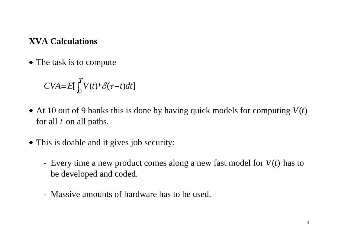
XVA Calculations

The task is to compute

0[ ( ) ( ) ]

TCVA E V t t dt

At 10 out of 9 banks this is done by having quick models for computing ( )V t

for all t on all paths.

This is doable and it gives job security:

- Every time a new product comes along a new fast model for ( )V t has to

be developed and coded.

- Massive amounts of hardware has to be used.

3

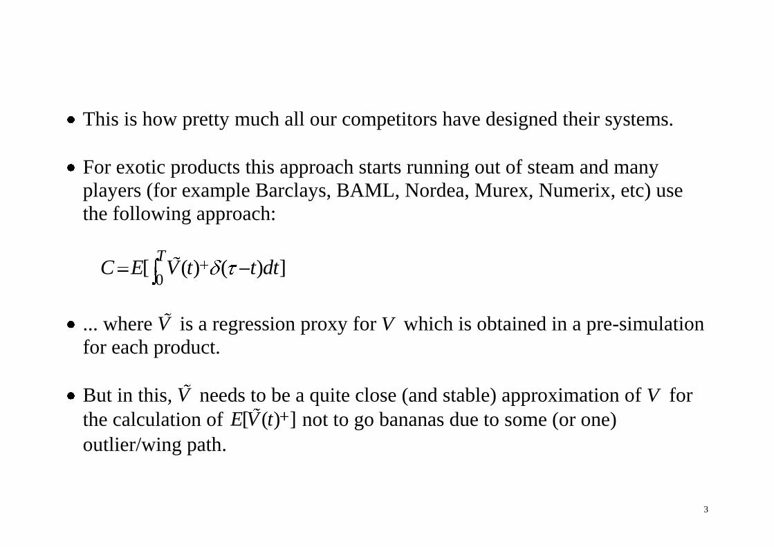
This is how pretty much all our competitors have designed their systems.

For exotic products this approach starts running out of steam and many

players (for example Barclays, BAML, Nordea, Murex, Numerix, etc) use

the following approach:

0[ ( ) ( ) ]

TC E V t t dt

... where V is a regression proxy for V which is obtained in a pre-simulation

for each product.

But in this, V needs to be a quite close (and stable) approximation of V for

the calculation of [ ( ) ]E V t not to go bananas due to some (or one)

outlier/wing path.

4

This in turn creates a lot of work on the choice of regression basis and

requires a lot of pre simulations => job security.

5

XVA Regressions

Our approach is based on using the following

0

0 ( ) 0

0 ( ) 0

0 ( ) 0

0 ( ) 0

[ ( ) ( ) ]

[ ( ) 1 ( ) ]

[ [ ( ) ]1 ( ) ]

[ ( )1 ( ) ]

[ ( 1 ( ) )

T

T

V t

regression proxy

T T

t t V tfuturecash flow

T T

t V t

u

V t

CVAnotional

C E V t t dt

E V t t dt

E E c u du t dt

E c u t dudt

E t dt0

( ) ]T

c u du

6

We note that the approximation V is only used for determining whether 0V

We also note that the approach gives a lower bound.

Effectively, what we are pricing is a contract that in case of counterparty

default and portfolio value is positive to us, pays us the future cash-flows of

the portfolio – not the present value.

Economically, there is no difference but we do not have to be able to

accurately value the portfolio at default time – only assess whether the

portfolio has positive value to us and then simulate the cash flows.

The first advantage of this is that the approximation V doesn’t have to be

accurate on the entire state space, it only needs to be accurate around 0V .

7

This in turn means that we do not have to work very hard on the regressions

or use a very high number of pre simulations.

We usually use 256-1024 pre simulations for the regressions. We have seen

competitors that use 65,536 simulations in the regressions – on their GPUs.

8

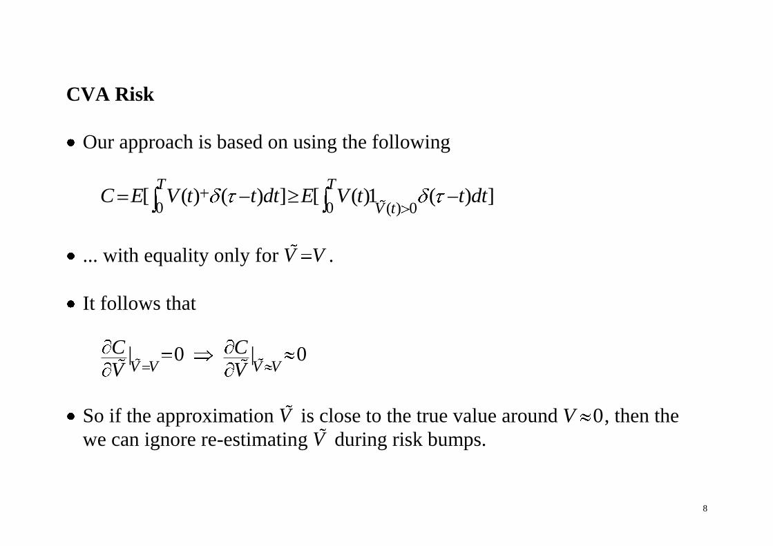
CVA Risk

Our approach is based on using the following

0 0 ( ) 0[ ( ) ( ) ] [ ( )1 ( ) ]

T T

V tC E V t t dt E V t t dt

... with equality only for V V .

It follows that

| 0 | 0V V V V

C CV V

So if the approximation V is close to the true value around 0V , then the

we can ignore re-estimating V during risk bumps.

9

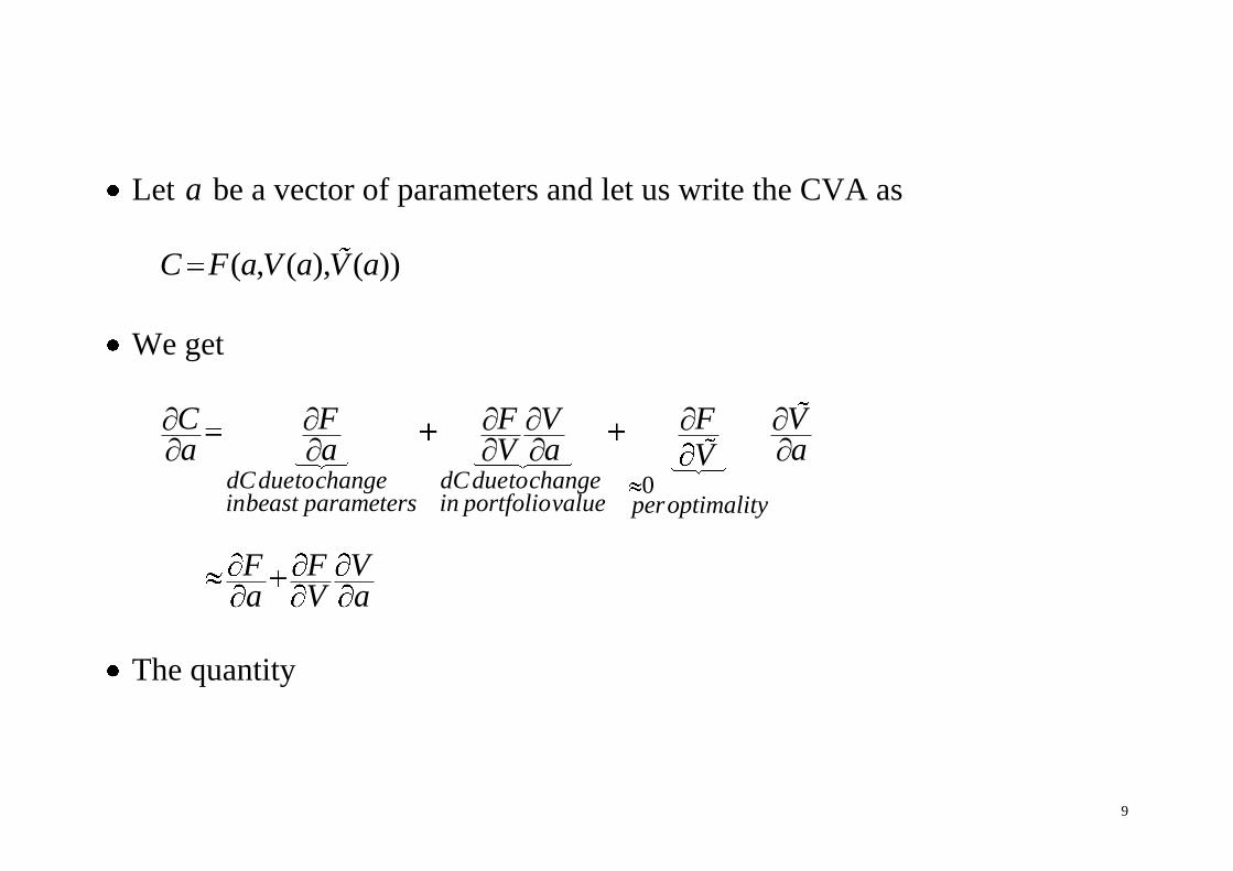
Let a be a vector of parameters and let us write the CVA as

( , ( ), ( ))C F a V a V a

We get

0dCduetochange dCduetochangeinbeast parameters in portfoliovalue peroptimality

C F F V F Va a V a aV

F F Va V a

The quantity

10

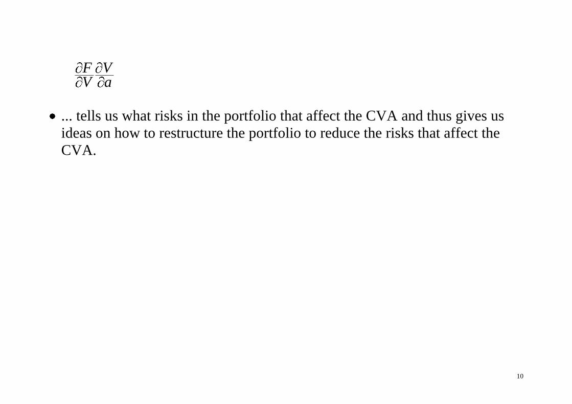
F VV a

... tells us what risks in the portfolio that affect the CVA and thus gives us

ideas on how to restructure the portfolio to reduce the risks that affect the

CVA.

11

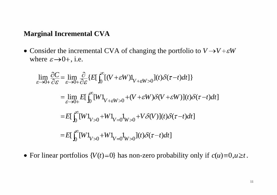
Marginal Incremental CVA

Consider the incremental CVA of changing the portfolio to V V W

where 0 , i.e.

000 0

000

0 0 00

0 0 00

lim lim { [ [( )1 ]( ) ( ) ]}

lim [ [ 1 ( ) ( )]( ) ( ) ]

[ [ 1 1 1 ( )]( ) ( ) ]

[ [ 1 1 1 ]( ) ( ) ]

V W

V W

V V W

V V W

C E V W t t dt

E W V W V W t t dt

E W W V V t t dt

E W W t t dt

For linear portfolios { ( ) 0}V t has non-zero probability only if ( ) 0,c u u t .

12

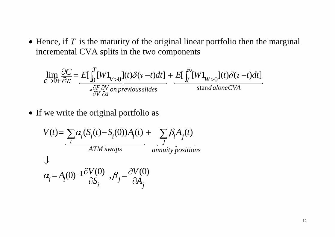
Hence, if T is the maturity of the original linear portfolio then the marginal

incremental CVA splits in the two components

0 000tan

lim [ [ 1 ]( ) ( ) ] [ [ 1 ]( ) ( ) ]T

V WTF V s d aloneCVAon previousslidesV a

C E W t t dt E W t t dt

If we write the original portfolio as

1

( ) ( ( ) (0)) ( ) ( )

(0) (0)(0) ,

i i i i i ji j

ATM swaps annuity positions

i i ji j

V t S t S A t A t

V VAS A

13

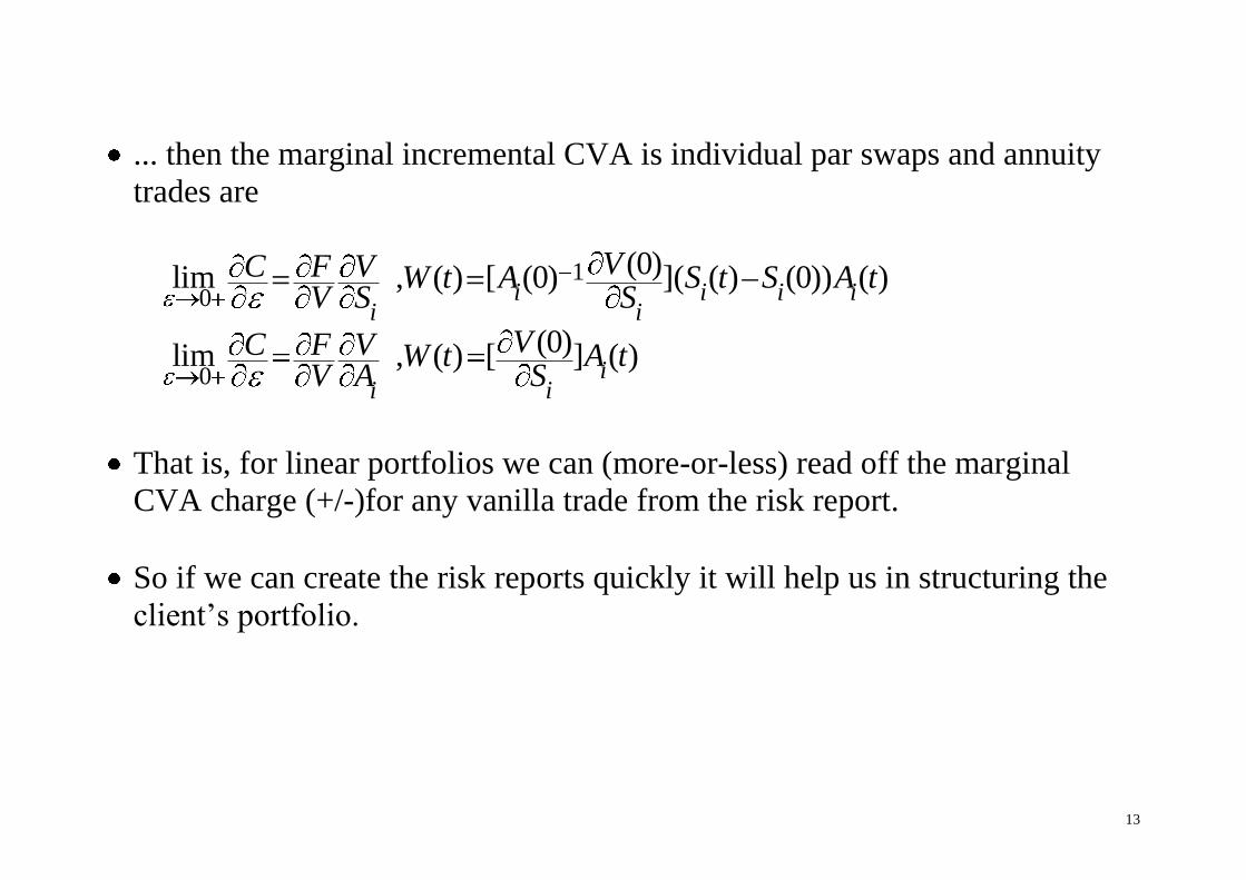
... then the marginal incremental CVA is individual par swaps and annuity

trades are

10

0

(0)lim , ( ) [ (0) ]( ( ) (0)) ( )

(0)lim , ( ) [ ] ( )

i i i ii i

ii i

VC F V W t A S t S A tV S S

VC F V W t A tV A S

That is, for linear portfolios we can (more-or-less) read off the marginal

CVA charge (+/-)for any vanilla trade from the risk report.

So if we can create the risk reports quickly it will help us in structuring the

client’s portfolio.

14

Jive Infrastructure

One of the primary advantages of the regression approach is that it fits

(extremely) nice with the Danske infrastructure.

Danske has since 2008 used a scripting language called Jive for all valuation

in the quant library SuperFly.

This includes everything that we trades from completely simple stuff such as

FX forwards to exotic equity options.

Vanilla trades typically get on-the-fly Ottomatically converted to Jive cash

flows.

We can reuse existing Ottomatic machinery that Jives the cash flows, we just

need to modify the discounting of the simulated Jive cash flows.

15

Jive Overlay

Note that there is a whole collection of different things that you want to

compute once you can compute the CVA.

After that you want the CVA, DVA, FVA, collateral options, CVA on

collateralised counterparties, VaR, VaR on CVA, etc etc etc

The new exotic are not the promised cash flows – but how you discount

them.

This means that it makes a lot of sense give all xVA calculations a Jive

interface.

This is what we have done with the sJiveCva() function.

16

pos event

S rf_var regress()

S cva_ntl = cva_ntl + (1-recovery(enddate(), enddate(), SG))*(index(startdate(), startdate(), SG) - index(enddate(), enddate(), SG))*(proxy(RF_VAR)>0)

pay var pay ntl

rf_var 1

cva_var cva_ntl

17

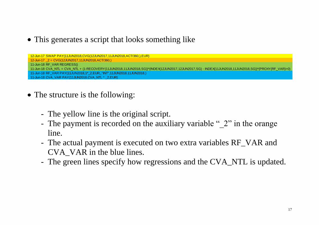
This generates a script that looks something like

The structure is the following:

- The yellow line is the original script.

- The payment is recorded on the auxiliary variable “_2” in the orange

line.

- The actual payment is executed on two extra variables RF_VAR and

CVA_VAR in the blue lines.

- The green lines specify how regressions and the CVA_NTL is updated.

12-Jun-17 SWAP PAY(11JUN2018,CVG(12JUN2017,11JUN2018,ACT/360,),EUR)

12-Jun-17 _2 = CVG(12JUN2017,11JUN2018,ACT/360,)

11-Jun-18 RF_VAR REGRESS()

11-Jun-18 CVA_NTL = CVA_NTL + (1-RECOVERY(11JUN2018,11JUN2018,SG))*(INDEX(12JUN2017,12JUN2017,SG) - INDEX(11JUN2018,11JUN2018,SG))*(PROXY(RF_VAR)>0)

11-Jun-18 RF_VAR PAY(11JUN2018,1*_2,EUR,,"INT",11JUN2018,11JUN2018,)

11-Jun-18 CVA_VAR PAY(11JUN2018,CVA_NTL * _2,EUR)

18

Yellow, orange (with new var name) and blue lines are repeated for every

payment.

Green lines for other commands are inserted as specified by the user.

Note that we can use existing Otto machinery – we do not need to clone Otto

to write the regression statements etc.

The industrial kwant at work again!

This methodology creates more lines of Jive to execute but it does not carry

a higher overhead in terms market data that needs to be generated and stored

during regressions.

It ensures that the we correctly handle the accumulation of the CVA notional

between fixing and payment.

19

...which is also useful for collateral options.

20

Regression Variables

The regression variables are supplied by the Beast. Standard configuration

is:

- 1y and 30y zero rates for each currency.

- Discount basis factor for each currency.

- Fx rate for each currency pair.

- Stochastic volatility factors.

The actual zero rates used can be changed on the MFCs.

The generated regression polynomial is only 1st order but can be increased

by the user on Beast level.

21

Note, however, that doing so can be criminal as the number of regression

coefficients to be estimated will be squared. I.e. in this case (many) more pre

simulations could be needed.

Simulation:

- Number of pre simulations .NUM PRE SIM = 256

- Number of simulations .NUM BATCH*.NUM SIM = 8*256

22

Compression

Generally, the number of event dates and the amount of model data will

increase linearly with the trade count and the length of the trades.

For large portfolios we get to a situation where every date between here and

maturity has to be simulated to and fixings have to be stored on.

This is particularly a problem for the regressions because for these, bundles

of paths need to be stored in the memory of the computer.

However, nothing we compute here really needs daily resolution on the

fixings, so it seems natural to try to standardise the dates that we simulate

and the data that is being stored.

23

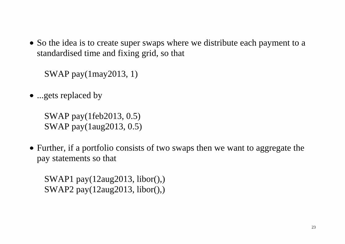
So the idea is to create super swaps where we distribute each payment to a

standardised time and fixing grid, so that

SWAP pay(1may2013, 1)

...gets replaced by

SWAP pay(1feb2013, 0.5)

SWAP pay(1aug2013, 0.5)

Further, if a portfolio consists of two swaps then we want to aggregate the

pay statements so that

SWAP1 pay(12aug2013, libor(),)

SWAP2 pay(12aug2013, libor(),)

24

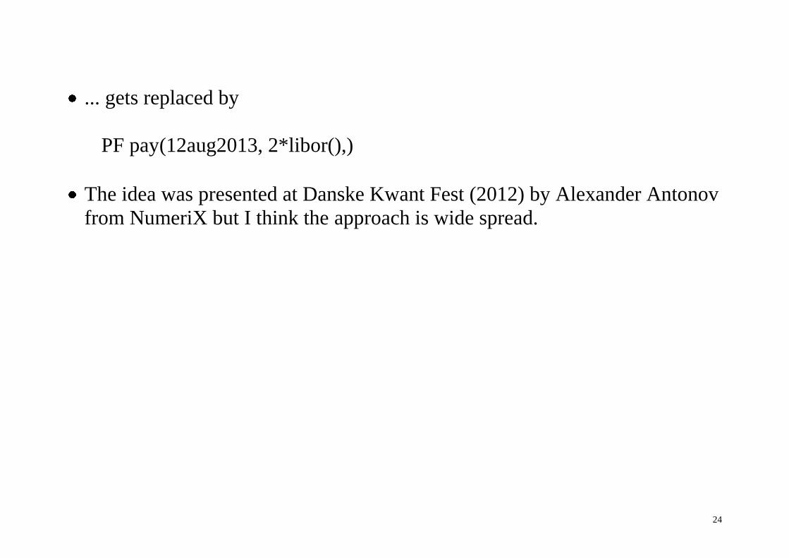
... gets replaced by

PF pay(12aug2013, 2*libor(),)

The idea was presented at Danske Kwant Fest (2012) by Alexander Antonov

from NumeriX but I think the approach is wide spread.

25

Jive Compression

Again, this task can be done without Otto intervention.

First, we note that if a variable appears anywhere on the Right-Hand-Side in

a Jive script, like VAR2 in

VAR1 pay(12aug2014, VAR2)

or

VAR3 = 3*VAR2

... then the payments of VAR2 cannot be compressed into payments on PF.

26

The visitor for analysing a Jive script for which variables can be compressed

on is only 100 lines of code.

27

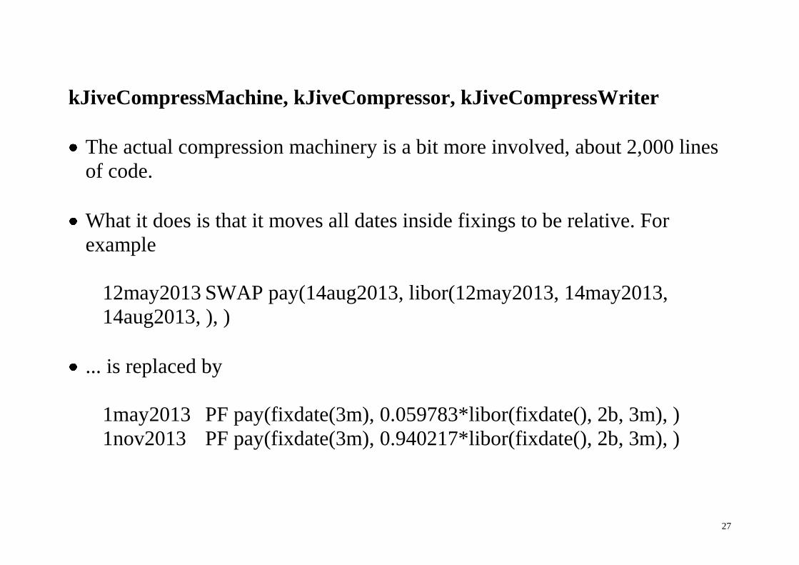
kJiveCompressMachine, kJiveCompressor, kJiveCompressWriter

The actual compression machinery is a bit more involved, about 2,000 lines

of code.

What it does is that it moves all dates inside fixings to be relative. For

example

12may2013 SWAP pay(14aug2013, libor(12may2013, 14may2013,

14aug2013, ), )

... is replaced by

1may2013 PF pay(fixdate(3m), 0.059783*libor(fixdate(), 2b, 3m), )

1nov2013 PF pay(fixdate(3m), 0.940217*libor(fixdate(), 2b, 3m), )

28

It is implemented as a special Jive evaluator that do +-*/ operations on

map<string,double> rather than on double.

29

xVA Calculation Summary

Regressions are good but they have to be applied sensibly.

Using the (near) optimality of the regressions largely simplify risk and

marginal CVA calculations.

Jive is the star of the show here.

The SuperFly use of Jive for all model/product relation simplifies the CVA

job greatly.

By use of Jive we are able to strap on the xVA calculations in a user-

configurable way.

Jive also enables compression in a relatively painless way.

30

Compression is generally necessary even for 64 bit machinery.

... and vice-versa: Some portfolios are so big that we need to run them on 64

bit machines even after compression.

*LIVE* EXAMPLE.