18
| Date post: | 12-Aug-2015 |
| Category: |
Technology |
| Upload: | akisato-kimura |
| View: | 130 times |
| Download: | 1 times |

Paper to read
CVPR2015 (poster)
2

1-page summary
• A method for refining a pre-trained random forest– Comparable to RF with much more nodes of decision trees– Better than RF with the same size of decision trees
3
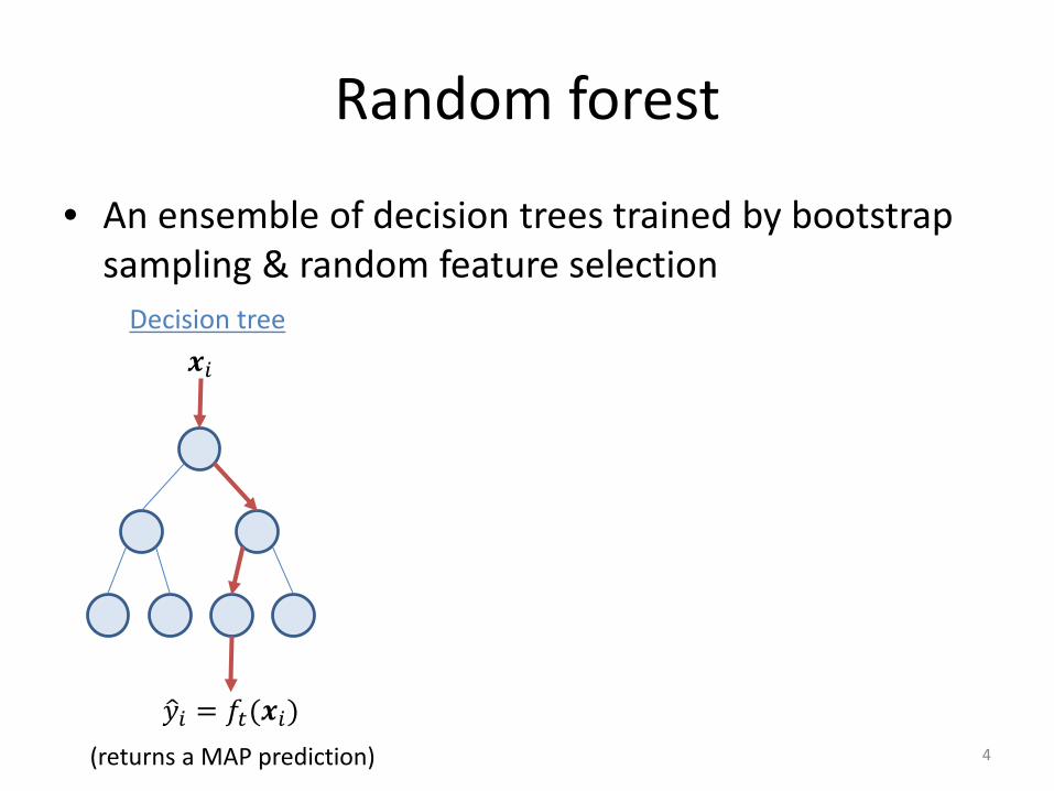
Random forest
• An ensemble of decision trees trained by bootstrap sampling & random feature selection
Decision tree𝒙𝒙𝑖𝑖
�𝑦𝑦𝑖𝑖 = 𝑓𝑓𝑡𝑡(𝒙𝒙𝑖𝑖)(returns a MAP prediction) 4
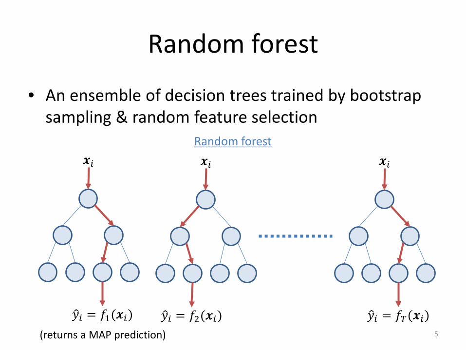
Random forest
• An ensemble of decision trees trained by bootstrap sampling & random feature selection
𝒙𝒙𝑖𝑖
�𝑦𝑦𝑖𝑖 = 𝑓𝑓1(𝒙𝒙𝑖𝑖)(returns a MAP prediction)
𝒙𝒙𝑖𝑖
�𝑦𝑦𝑖𝑖 = 𝑓𝑓2(𝒙𝒙𝑖𝑖)
𝒙𝒙𝑖𝑖
�𝑦𝑦𝑖𝑖 = 𝑓𝑓𝑇𝑇(𝒙𝒙𝑖𝑖)
Random forest
5
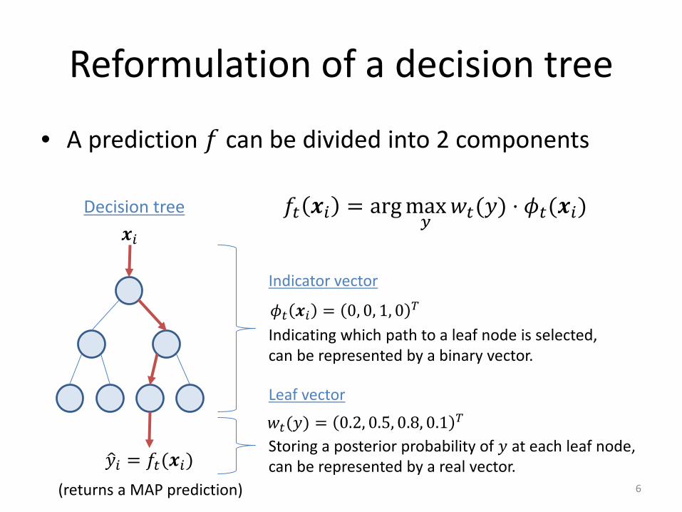
Reformulation of a decision tree
• A prediction 𝑓𝑓 can be divided into 2 components
Decision tree𝒙𝒙𝑖𝑖
�𝑦𝑦𝑖𝑖 = 𝑓𝑓𝑡𝑡(𝒙𝒙𝑖𝑖)(returns a MAP prediction)
𝜙𝜙𝑡𝑡 𝒙𝒙𝑖𝑖 = 0, 0, 1, 0 𝑇𝑇
Indicating which path to a leaf node is selected,can be represented by a binary vector.
𝑤𝑤𝑡𝑡(𝑦𝑦) = 0.2, 0.5, 0.8, 0.1 𝑇𝑇
Storing a posterior probability of 𝑦𝑦 at each leaf node,can be represented by a real vector.
𝑓𝑓𝑡𝑡 𝒙𝒙𝑖𝑖 = arg max𝑦𝑦
𝑤𝑤𝑡𝑡(𝑦𝑦) ⋅ 𝜙𝜙𝑡𝑡(𝒙𝒙𝑖𝑖)
Indicator vector
Leaf vector
6
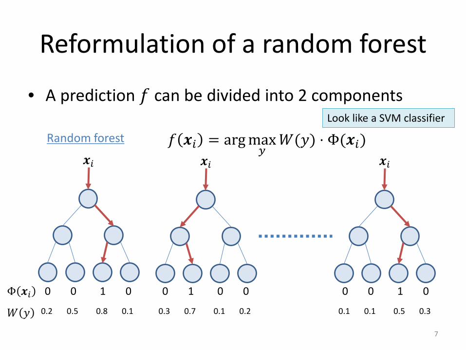
Reformulation of a random forest
• A prediction 𝑓𝑓 can be divided into 2 components
𝒙𝒙𝑖𝑖 𝒙𝒙𝑖𝑖 𝒙𝒙𝑖𝑖
0 0 1 0 0 1 0 0 0 0 1 0Φ 𝒙𝒙𝑖𝑖0.2 0.5 0.8 0.1 0.3 0.7 0.1 0.2 0.1 0.1 0.5 0.3𝑊𝑊 𝑦𝑦
Random forest 𝑓𝑓 𝒙𝒙𝑖𝑖 = arg max𝑦𝑦
𝑊𝑊(𝑦𝑦) ⋅ Φ(𝒙𝒙𝑖𝑖)
7
Look like a SVM classifier

Global refinement
• Optimize a leaf vector (weights) 𝑊𝑊(𝑦𝑦),while maintaining the indicator vector (structure) Φ(𝑥𝑥)
𝒙𝒙𝑖𝑖 𝒙𝒙𝑖𝑖 𝒙𝒙𝑖𝑖
0 0 1 0 0 1 0 0 0 0 1 0Φ 𝒙𝒙𝑖𝑖0.1 0.3 0.9 0.1 0.1 0.8 0.1 0.2 0.1 0.1 0.7 0.1�𝑊𝑊 𝑦𝑦
Random forest 𝑓𝑓 𝒙𝒙𝑖𝑖 = arg max𝑦𝑦
𝑊𝑊(𝑦𝑦) ⋅ Φ(𝒙𝒙𝑖𝑖)
8

Global refinement
• Optimize a leaf vector (weights) 𝑊𝑊(𝑦𝑦),while maintaining the indicator vector (structure) Φ(𝑥𝑥)
𝒙𝒙𝑖𝑖 𝒙𝒙𝑖𝑖 𝒙𝒙𝑖𝑖
0 0 1 0 0 1 0 0 0 0 1 0Φ 𝒙𝒙𝑖𝑖0.1 0.3 0.9 0.1 0.1 0.8 0.1 0.2 0.1 0.1 0.7 0.1�𝑊𝑊 𝑦𝑦
Random forest 𝑓𝑓 𝒙𝒙𝑖𝑖 = arg max𝑦𝑦
𝑊𝑊(𝑦𝑦) ⋅ Φ(𝒙𝒙𝑖𝑖)
This optimization can be regarded as a linear classification problem,where an indicator vector Φ(𝒙𝒙) is a new representation of a sample 𝒙𝒙.
[Note] In standard random forest, the trees are independently optimized.This optimization effectively utilizes complementary information among trees.
9

Global refinement
• Optimize a leaf vector (weights) 𝑊𝑊(𝑦𝑦),while maintaining the indicator vector (structure) Φ(𝑥𝑥)
𝒙𝒙𝑖𝑖 𝒙𝒙𝑖𝑖 𝒙𝒙𝑖𝑖
0 0 1 0 0 1 0 0 0 0 1 0Φ 𝒙𝒙𝑖𝑖0.1 0.3 0.9 0.1 0.1 0.8 0.1 0.2 0.1 0.1 0.7 0.1�𝑊𝑊 𝑦𝑦
Random forest 𝑓𝑓 𝒙𝒙𝑖𝑖 = arg max𝑦𝑦
𝑊𝑊(𝑦𝑦) ⋅ Φ(𝒙𝒙𝑖𝑖)
This optimization can be regarded as a linear classification problem,where an indicator vector Φ(𝒙𝒙) is a new representation of a sample 𝒙𝒙.
A sample Φ(𝑥𝑥) is highly sparse Liblinear well suits this problem.
It can be easily extended to a regression problem.
10
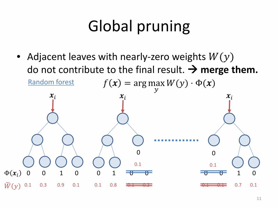
Global pruning
• Adjacent leaves with nearly-zero weights 𝑊𝑊(𝑦𝑦)do not contribute to the final result. merge them.
𝒙𝒙𝑖𝑖 𝒙𝒙𝑖𝑖 𝒙𝒙𝑖𝑖
0 0 1 0 0 1 0 0 0 0 1 0Φ 𝒙𝒙𝑖𝑖0.1 0.3 0.9 0.1 0.1 0.8 0.1 0.2 0.1 0.1 0.7 0.1�𝑊𝑊 𝑦𝑦
Random forest 𝑓𝑓 𝒙𝒙 = arg max𝑦𝑦
𝑊𝑊(𝑦𝑦) ⋅ Φ(𝒙𝒙)
0
0.1
0
0.1
11
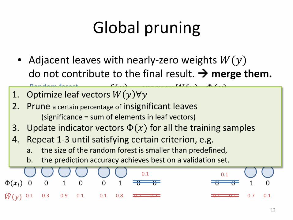
Global pruning
• Adjacent leaves with nearly-zero weights 𝑊𝑊(𝑦𝑦)do not contribute to the final result. merge them.
𝒙𝒙𝑖𝑖 𝒙𝒙𝑖𝑖 𝒙𝒙𝑖𝑖
0 0 1 0 0 1 0 0 0 0 1 0Φ 𝒙𝒙𝑖𝑖0.1 0.3 0.9 0.1 0.1 0.8 0.1 0.2 0.1 0.1 0.7 0.1�𝑊𝑊 𝑦𝑦
Random forest 𝑓𝑓 𝒙𝒙 = arg max𝑦𝑦
𝑊𝑊(𝑦𝑦) ⋅ Φ(𝒙𝒙)
0
0.1
0
0.1
1. Optimize leaf vectors 𝑊𝑊 𝑦𝑦 ∀𝑦𝑦2. Prune a certain percentage of insignificant leaves
(significance = sum of elements in leaf vectors)3. Update indicator vectors Φ(𝑥𝑥) for all the training samples4. Repeat 1-3 until satisfying certain criterion, e.g.
a. the size of the random forest is smaller than predefined,b. the prediction accuracy achieves best on a validation set.
12

Data sets for experiments
13

Experimental results
• ADF/ARF - alternating decision (regression) forest [Schulter+ ICCV13]• Refined-A - Proposed method with the “accuracy” criterion• Refined-E - Proposed method with “over-pruning”
(Accuracy is comparable to the original RF, but the size is much smaller.)• Metrics - Error rate for classification, RMSE for regression.• # trees = 100, max. depth = 10, 15 or 25 depending on the size of the training data.• 60% for training, 40% for testing. 14

Parameter analysis
• The proposed method achieved better performancesthan RFs with the same tree parameters (e.g. the number and depth of trees)
15
(for MNIST data)

Parameter analysis
• The proposed method accelerates both training and testing steps
16
(for MNIST data)
Number of dimensions used on each node splitting
Number of samples used in each decision tree
Best for RFBest for proposed
Time for testingfast slow Time for trainingfast slow
Less sensitive More samples needed
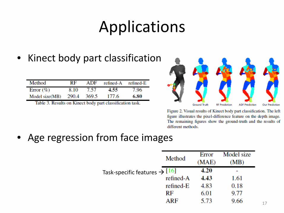
Applications
• Kinect body part classification
• Age regression from face images
17
Task-specific features

Last words
• Simple, easy to implement, but effective• Can be applicable to other classifiers
18


