Cymcap Manual

February 2007

CYMCAP 4.6 for Windows

Copyright CYME International T&D Inc.

All Rights Reserved

This publication, or parts thereof, may not be reproduced in any form, by any method, for any purpose. CYME International T&D makes no warranty, either expressed or implied, including but not limited to any implied warranties of merchantability or fitness for a particular purpose, regarding these materials and makes such materials available solely on an "as-is" basis. In no event shall CYME International T&D be liable to anyone for special, collateral, incidental, or consequential damages in connection with or arising out of purchase or use of these materials. The sole and exclusive liability to CYME International T&D, regardless of the form of action, shall not exceed the purchase price of the materials described herein. CYME International T&D reserves the right to revise and improve its products as it sees fit. This publication describes the state of this product at the time of its publication, and may not reflect the product at all times in the future. The software described in this document is furnished under a license agreement. CYME International T&D Inc. 67 South Bedford Street, Suite 201 East Burlington, MA 01803-5177 1-800-361-3627 (781) 229-0269 FAX: (781) 229-2336 International and Canada: 1485 Roberval, Suite 104 St. Bruno QC J3V 3P8 Canada (450) 461-3655 Fax: (450) 461-0966

Internet : http://www.cyme.com E-mail : [email protected]

Windows 98 and Windows NT, 2000 & XP are registered trademarks of Microsoft. Autocad is a trademark of Autodesk Inc.

NOTICE The computer programs described in this manual were developed jointly by CYME International T&D Inc., Ontario Hydro and McMaster University under the auspices of the Canadian Electricity Association (CEA). Neither CYME International T&D, Ontario Hydro, McMaster University, CEA, nor any person acting on their behalf: (a) makes any warranty, express or implied of any kind with regard to the use of the computer programs, the documentation and any information, method or process disclosed therein, or that such use may not infringe privately owned rights; or (b) assumes any liabilities with regard to the use of, or damages resulting from the use of the programs or other information contained in this document. The software described in this document is furnished under a license agreement.

CYMCAP for Windows

TABLE OF CONTENTS I

Table of Contents

Chapter 1 Getting Started ..............................................................................1 1.1 Overview of CYMCAP ..................................................................................1 1.2 Software and hardware requirements ..........................................................2 1.3 Installing CYMCAP for Windows ..................................................................2

1.3.1 Installation steps – From a CD..........................................................2 1.3.2 Installation steps – From a downloaded file......................................3 1.3.3 Setting up the protection key.............................................................3 1.3.4 Windows Settings..............................................................................3

1.4 The contents of CYMCAP ............................................................................4 1.4.1 CYMCAP Graphical User Interface...................................................5 1.4.2 The CYMCAP libraries and utilities – an overview............................5 1.4.3 Populating the CYMCAP libraries .....................................................7

1.5 What you should know about running studies with CYMCAP......................8

Chapter 2 The Cable Library ..........................................................................9 2.1 Introduction ...................................................................................................9

2.1.1 Cable data in studies.........................................................................9 2.2 Cable library Navigator window..................................................................10

2.2.1 Cable library window commands ....................................................11 2.2.2 Cable library pop-up menu..............................................................12

2.3 Cable design data window elements..........................................................13 2.4 Steps to create a new cable .......................................................................16 2.5 Cable components, materials and construction .........................................17

2.5.1 Conductor data................................................................................18 2.5.2 Conductor shield data .....................................................................21 2.5.3 Insulation data .................................................................................22 2.5.4 Insulation screen .............................................................................23 2.5.5 Sheath .............................................................................................24 2.5.6 Sheath Reinforcing Material............................................................24 2.5.7 Skid wires (for pipe type cables only) .............................................25 2.5.8 Concentric neutral wires..................................................................25 2.5.9 Armour/Reinforcing tape .................................................................26 2.5.10 Armour Bedding/Armour Serving ....................................................27 2.5.11 Jacket, oversheath and pipe coating material.................................28

2.6 Creating a new cable - Example.................................................................29 2.7 Useful considerations .................................................................................35

2.7.1 Cable layers ....................................................................................35 2.7.2 Particular modeling..........................................................................35 2.7.3 SL-type cables.................................................................................36 2.7.4 Custom materials and thermal capacitances ..................................36

2.8 Filter Editor .................................................................................................37

Chapter 3 The Ductbank Library..................................................................39 3.1 Introduction .................................................................................................39 3.2 Ductbank library management....................................................................39

3.2.1 Creating a new duct bank. An illustrative example. ........................40

Chapter 4 Load-Curves/Heat Source Curves and Shape Libraries ..........43 4.1 Introduction .................................................................................................43

4.1.1 Curves and Shapes.........................................................................43 4.2 Shape Library management .......................................................................44

CYMCAP for Windows

II TABLE OF CONTENTS

4.2.1 Creating a new shape – An Illustrative example.............................45 4.2.2 Shifting a shape – An illustrative example ......................................47

4.3 Load and Heat Source Libraries Management...........................................49 4.3.1 Expanding and collapsing the curves .............................................50 4.3.2 Curves libraries command buttons .................................................52 4.3.3 Create a Load Curve using existing shapes – An illustrative example ......................................................................................................52 4.3.4 Load Curve from field-recorded data ..............................................57

Chapter 5 Steady State Thermal Analysis ..................................................61 5.1 General .......................................................................................................61 5.2 Methodology and computational standards................................................61 5.3 Accuracy of CYMCAP and References......................................................64

5.3.1 References ......................................................................................66 5.4 Studies and executions ..............................................................................66 5.5 Library of studies and executions ...............................................................67

5.5.1 Study library pop-up menu ..............................................................68 5.6 Creating a study..........................................................................................72 5.7 Analysis options..........................................................................................74 5.8 Steady state analysis..................................................................................75

5.8.1 General data for the installation ......................................................76 5.8.2 Cable Installation data.....................................................................82 5.8.3 Specific cable installation data ........................................................83

5.9 Cable Library data and executions .............................................................89 5.10 Steady state thermal analysis, Example 1: Cables in a duct bank.............90

5.10.1 Defining a new study and a new execution.....................................91 5.10.2 Setting the steady state analysis solution Option ...........................92 5.10.3 Execution speed bar and associated command buttons ................93 5.10.4 Defining standard and/or non-standard duct banks........................95 5.10.5 Importing a duct bank from the Library ...........................................96 5.10.6 Defining the general installation data and setup .............................97 5.10.7 Defining the cable installation data .................................................98 5.10.8 Rearranging the cables in the proper ducts ..................................100

5.11 A study case for dissimilar directly buried cables.....................................101 5.11.1 Define a new execution using an existing one as template ..........101 5.11.2 Modify the solution option from the CYMCAP menu.....................102 5.11.3 Enter a group of cables using absolute coordinates.....................103 5.11.4 Enter a trefoil formation using relative coordinates.......................103 5.11.5 Specify a “fixed ampacity circuit”...................................................105 5.11.6 Convergence and the Selection of Reference Circuit...................106 5.11.7 Specify a heat source included in the installation .........................107

5.12 Specific installation data ...........................................................................108 5.13 Results Reporting .....................................................................................108 5.14 Steady-state results labels .......................................................................109

5.14.1 View/hide labels ............................................................................110 5.14.2 Label grid editor.............................................................................111 5.14.3 Select/move/align labels ...............................................................111 5.14.4 Change the connection line between the cable and its associated label 113 5.14.5 Change the properties of a label ...................................................113 5.14.6 Reset all labels to their default positions.......................................114 5.14.7 Keep all labels positions permanently...........................................115

5.15 Viewing the graphical ampacity reports by mouse selection....................116 5.16 Tabular Reports ........................................................................................118 5.17 MS Excel (Final) Report............................................................................118

5.17.1 The Electrical Tab..........................................................................121

CYMCAP for Windows

TABLE OF CONTENTS III

5.18 Opening more than one executions simultaneously ................................124 5.19 Working with more than one executions simultaneously .........................127

5.19.1 Submitting more than one executions simultaneously..................127

Chapter 6 Transient Analysis.....................................................................129 6.1 General .....................................................................................................129 6.2 Preliminary considerations .......................................................................129 6.3 Transient analysis options ........................................................................130

6.3.1 Solve for Ampacity Given Time and Temperature ........................130 6.3.2 Solve for Temperature given Time and Ampacity.........................131 6.3.3 Solve for Time given Ampacity and Temperature.........................132 6.3.4 Ampacity as a function of Temperature ........................................133 6.3.5 Ampacity as a function of Time .....................................................133 6.3.6 Temperature as a function of Time ...............................................134

6.4 How to proceed for a transient analysis ...................................................135 6.5 Informing CYMCAP that a transient analysis is to be performed .............135 6.6 Example and Illustrations .........................................................................136

6.6.1 Case description and illustrations .................................................136 6.6.2 Specify the transient analysis option.............................................137 6.6.3 Specify the data for the transient analysis option .........................137 6.6.4 Assign Loads to Cables ................................................................138 6.6.5 Submit the simulation ....................................................................139 6.6.6 Generate the reports .....................................................................140 6.6.7 Change the color of the curves for the transient reports...............142 6.6.8 Trace the transients results with the mouse .................................142

Chapter 7 Approximate Temperature Field...............................................145 7.1 Introduction ...............................................................................................145 7.2 Scopes and Limitations ............................................................................146 7.3 Customizing the Isotherms .......................................................................147 7.4 Automatic Design of Backfills/Duct Banks................................................149

Chapter 8 The Sensitivity Analysis Option of CYMCAP ..........................153

Chapter 9 The CYMCAP Menu ...................................................................157 9.1 Overview of the CYMCAP Menu ..............................................................157 9.2 The Files menu .........................................................................................157 9.3 The Windows menu..................................................................................158 9.4 The CYMCAP menu for opened executions ............................................158 9.5 The File menu - Execution........................................................................158 9.6 The Edit menu - Execution .......................................................................159 9.7 The View menu - Execution......................................................................159 9.8 The Options menu - Execution .................................................................160

9.8.1 Simulation control parameters ......................................................162 9.9 Designate the Unit System for the session ..............................................163 9.10 Designate the AC system frequency for the session ...............................163 9.11 Designate AC conductor resistance values..............................................163

Chapter 10 CYMCAP Utilities.......................................................................165 10.1 Introduction ...............................................................................................165 10.2 Designate the working directory for CYMCAP .........................................165 10.3 Backup the contents of the Working directory to another directory .........166 10.4 Append a database to another database .................................................166 10.5 Restore from floppy disk to a directory on the hard-disk..........................167 10.6 Tag specific items from the Libraries........................................................167 10.7 Copy selected items to a given data base................................................168

CYMCAP for Windows

IV TABLE OF CONTENTS

Chapter 11 Defaults for Various Types of Cables ......................................171 11.1 Defaults – Overview..................................................................................171 11.2 Concentric neutral cables .........................................................................171 11.3 Extruded dielectric cables.........................................................................173 11.4 Low pressure oil filled cables (Type 3) .....................................................174 11.5 High pressure oil (gas) filled cables .........................................................175 11.6 Sheath related defaults.............................................................................177 11.7 Armour related defaults ............................................................................178

11.7.1 Three core cables..........................................................................178

CYMCAP for Windows

CHAPTER 1 –- GETTING STARTED 1

Chapter 1 Getting Started

1.1 Overview of CYMCAP

The determination of the maximum current that a cable can sustain without deterioration of any of its electrical and/or mechanical properties has always been of prime interest to engineers and constitutes an important design parameter for both system planning and operations.

Accurate ampacity studies help maximizing the benefits from the considerable capital investment associated with cable installations. Also they help to increase system reliability and the proper utilization of the installed equipment.

CYMCAP is a Windows-based software designed to perform thermal analyses. It addresses both steady state and transient thermal cable rating. These thermal analyses pertain to temperature rise and/or ampacity calculations using the analytical techniques described by Neher-McGrath and the IEC 287 and IEC 853 International standards. More details on the implemented methods and the validation made to CYMCAP can be found in section 5.2 Methodology and computational standards.

CYMCAP features four additional optional analysis modules, the capabilities of which are covered in a separate manual. The modules are:

The CYMCAP/OPT Duct Bank Optimizer to determine the placement of several circuits within a duct bank so that certain optimal criteria are fulfilled.

The Multiple Duct Banks module (MDB) to determine the steady state ampacity of cables when they are placed in several duct banks and/or backfills in the same installation.

The CYMCAP/SCR Short Circuit Cable Rating (SCR) module dedicated to the calculation of the adiabatic and non-adiabatic short-circuit ratings.

The Cables in Tunnels Module to determine the temperature, steady state, cyclic and transient ampacity of cables installed in unventilated tunnels.

The Magnetic Fields Module. Once an ampacity or a temperature run has been performed, the module computes the magnetic flux density at any point on or above the ground for an underground cable installation using the current computed or specified in the steady state simulation.

CYMCAP for Windows

2 CHAPTER 1- GETTING STARTED

1.2 Software and hardware requirements

CYMCAP is a 32-bit application, runs on IBM PC or compatible personal computers and can be used with Windows NT and Windows XP operating systems.

The minimum hardware requirements are: • A Pentium-based computer

• 32 MB RAM

• 10 MB free memory on the hard disk

• A Microsoft mouse or equivalent

• A color monitor with Super VGA and a graphic card supporting 256 colors or more

• Any printer or plotter supported by Windows

1.3 Installing CYMCAP for Windows

CYMCAP can be installed from a CD or downloaded from our web site at www.cyme.com/newversion.htm. In both cases, a password is needed for the application to be unpacked and installed. To obtain the proper password please contact CYME International.

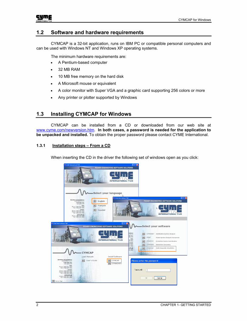
1.3.1 Installation steps – From a CD

When inserting the CD in the driver the following set of windows open as you click:

CYMCAP for Windows


Enter the password provided by CYME International T&D and CYMCAP will be installed in your computer.

1.3.2 Installation steps – From a downloaded file

When requesting the installation of CYMCAP from a file, you will get an email with instructions and the link to the download page together with the installation password. Clicking on the link www.cyme.com/newversion.htm will open the following screen.

Enter the information requested and click on the Download link. The password will be prompted and the installation will proceed.

1.3.3 Setting up the protection key

Once the application is unpacked and installed, the hardware lock, i.e. the protection key, is needed to operate it. The steps to setup the protection key are described in the Appendix titled Protection Key. The information can also be downloaded from: www.cyme.com/newversion.htm, scrolling down to the protection key section.

1.3.4 Windows Settings

For CYMCAP to function properly, you need to insure that you have the following settings on your machine:

• Screen resolution: CYMCAP needs that the screen resolution settings to be at least 800 x 600 pixels. The screen should be configured for Small (or Normal) Fonts size with a maximum of 96 dpi. Otherwise, some of the CYMCAP command buttons might not show.

• Regional settings: You need to use the Decimal Point. To set this, access your

Windows start menu (“Start”), select Control Panel, then Regional and Language Options (this can also be named Regional Options on your computer).

CYMCAP for Windows


1. Click the Number tab. In this window insure that: • ‘.’ is used as the Decimal Symbol. Click Apply and then

OK. 2. Click the Currency tab. In this window as well insure that:

• ‘.’ is used as the Decimal Symbol. Click Apply and then OK.

3. When you get back to the main Regional Options window, click OK to close the window.

1.4 The contents of CYMCAP

CYMCAP is equipped with calculating engines to perform Steady State, Cyclic and Transient analyses. These simulation programs produce the results and generate tabular and graphical reports.

Data for the steady state and transient simulators is provided through a Graphical User Interface (GUI) supported by the CYMCAP application libraries. These Libraries are the Study Library, the Cable Library, the Ductbank Library, the Shape Library, the Heat Source Library and the Load Curves Library.

The Study library serves to store and keep organized the different ampacity/temperature scenarios and specific data for the installation. This library has been specially designed to facilitate the study of “what if scenarios”. The Cable library is needed in all computations since it contains the details of the cable(s) construction. The Load Curves library and the Shape library are essential for transient thermal analysis. Similarly, the Ductbank library is needed for installations featuring duct banks and the Heat source Library is needed when the installation contains an external heat source in a transient thermal analysis.

CYMCAP for Windows


1.4.1 CYMCAP Graphical User Interface

When you open CYMCAP, the program’s main working window will be displayed with the CYMCAP Navigator overlaid on it. The description of the commands and use of the main window is described in the next subsections

The CYMCAP GUI Navigator provides access to the various libraries and to the Utilities window. The Navigator closes when you open a Study. You can re-display it by selecting the File > Open Navigator menu item in the main window, by pressing the F3 key or by clicking on the

icon

Each of the library windows is the subject of a separate chapter, starting at Chapter 3.

1.4.2 The CYMCAP libraries and utilities – an overview

Access to all CYMCAP libraries is independent, modular and does not rely on any predetermined sequence. The CYMCAP libraries and, therefore, all the application activities ranging from data management to actual simulation runs, are accessed through the CYMCAP Navigator.

Study Library This library contains all the studies performed by the application. CYMCAP relies on the concepts of "studies" and "executions" to organize study cases. A "study" can be viewed as a stand-alone scenario for thermal cable analysis, with several simulation alternatives (“what if scenarios”), named “executions”. A study normally pertains to a given installation exhibiting salient characteristics for the cable installation or the ambient conditions. Within a "study" you can define many "executions". An "execution" is used to describe a variant of the base case. See section 5.5 Library of studies and executions.

CYMCAP for Windows


Cable Library The Cable library is a database containing the detailed construction of various types of cables. The contents of the Cable library are used for both steady state and transient analyses. The Cable library, apart from being a database containing the various cable types, is equipped with a module that permits the definition of the cables themselves. Fairly detailed data is required to describe a cable, because the models used for the thermal representation of the cable rely heavily on the exact cable construction. This data is as essential, as the data describing the cable layout and the installation operating conditions.

CYMCAP offers the possibility to provide default cable dimensions based on generic cable construction characteristics, once the materials of the various cable components are defined. This facility is useful for preliminary cable studies but should not be interpreted as addressing all possible manufacturing practices. Chapter 2 is dedicated to describing the Cable library and its various functions, while the used default values for the cable components are given in Chapter 13.

Ductbank Library

The Ductbank library is a database containing the construction details of standard duct banks. A duct bank is a pre-constructed block containing several cable conduits. The purpose of the Duct bank library is to define the geometrical characteristics of these duct banks by specifying the total length, width, conduit number, duct spacing and specific duct diameter so that the information can be used as an integral part of any study for cables installed in duct banks.

The contents of the Ductbank library are used for both steady state and transient analyses. Duct bank geometrical characteristics are crucial in determining external thermal resistances. The Duct bank library, in addition from being a database containing the various duct bank types, is equipped with a module that permits the specification of new duct banks. Chapter 3 is dedicated to describing the Ductbank library and its various functions and facilities.

Heat Source Library

The Heat Source library is a database containing the transient thermal characteristics of external heat sources that may be present within a cable installation layout. External heat sources are deemed third party bodies that either emit or absorb heat depending on their temperature with reference to the ambient environment temperature. The heat source library contains the heat source curves that display the temporal variations of the heat source. Typical examples of heat sources are steam pipes and/or water pipes which temperature can vary as a function of time.

The Heat Source library is supported by another library, the Shape library and is used exclusively for transient thermal analyses. It is often important to include the presence of heat sources in the simulation, since heat sources alter considerably the temperature rise of the cables in an installation. The Heat Source library, apart from being a database, is equipped with a module that permits the definition of new heat source characteristics. In Chapter 4 we describe the Heat Source library and its various functions and facilities.

CYMCAP for Windows


Load Curves library

The Load Curves library is a database containing the description of the various patterns that the cable currents may exhibit as a function of time.

The Load Curves library is used exclusively for transient analysis and is supported by another library, the Shape library. The Load Curves library, apart from being a database, is equipped with a module that permits the construction of the Load Curves themselves. Load curve data is crucial for transient analysis. Load curves are defined in p.u. within the Load Curves library. The Load curve description does not contain actual ampere levels information. The “ampere-based” Load curves are interpreted during run time as the steady state value of the currents determined for the cables from the steady state thermal analysis. The description of the Load Curves library and its various functions are given in Chapter 4.

Shape Library The Shape library is not a stand-alone library. Instead, it is an auxiliary library dedicated to containing the building blocks for the entries of the “Heat Source” and the ”Load Curves” libraries. By definition, shapes are defined on a 24-hour basis and represent daily temporal variation patterns. Different shapes can be concatenated to produce weekly temporal profile variations.

Since, however, heat source shapes can only be invoked from the Heat Source library and load curves shapes can only be invoked from the “Load Curves” Library, there is no risk of confusion. It is essential to enter the required shapes in the Shape library first and then built the Heat Source curves/Load curves to be used for transient analysis. The Shape library, apart from being a database, is equipped with a module that permits the construction of new shapes as well.

Shapes are expressed in p.u. in order to give greater flexibility in describing temperature/heat flux levels for the heat sources and ampere loading levels for the load curves. The same entry format is used to describe both “Heat source” shapes and “load curve” shapes. Section 4.2 covers Shape Library management main functions.

It is emphasized again that all p.u. values entered in shapes and Load Curves/Heat Source Curves are expressed in p.u of the values these quantities assumed during steady state thermal analysis.

The CYMCAP Utilities are also accessible from the Navigator. The Utilities are used to manage the data files using powerful functions that help the user to keep projects organized in folders and subfolders or to perform data exchanges between users and computers. The CYMCAP Utilities are fully described in Chapter 9.

1.4.3 Populating the CYMCAP libraries

With the exception of the Study library, the CYMCAP libraries need to be populated before the application models any cable installation. Although typical entries are provided for most input data, it is mandatory; and it is the user’s responsibility to populate them with figures reflecting actual data. No supplied entry in the application libraries should be interpreted as being “typical” in any way.

To get accurate cable construction data, the CYMCAP user should contact the cable manufacturer providing the cables for the installation. The more detailed the information, the closer to reality the simulation would be. Dimensions for duct bank, backfills and burial depth should be available from the construction blueprints. Daily and weekly load curves should be available from the electrical system operator.

CYMCAP for Windows


1.5 What you should know about running studies with CYMCAP

The end result of using CYMCAP is to obtain temperatures and currents for the various cables contained in a given cable installation, operating under certain conditions. The following is a typical sequence of steps that are followed when using CYMCAP as an analysis tool.

1. Make sure that ALL the cables of the installation you are about to study are well defined construction-wise and dimension-wise. If this is not the case, try to obtain as much information as possible from the cable manufacturer.

2. Make sure that ALL the cable types that the simulation will use are entered in the CYMCAP Cable Library.

3. Make sure that the duct bank (if any) that the installation employs is entered in the Ductbank library. If the installation does not feature a duct bank, there is no need to populate the Ductbank library.

4. Make sure that the geometrical data of the installation you are about to study as well as the necessary simulation parameters (pipe dimensions, solar radiation intensities, bonding characteristics, ambient temperatures, thermal resistivities, etc.) are available and well defined. Use the graphical User Interface of CYMCAP to define the installation in detail.

5. Make certain that you clearly specify the type of analysis option you wish to perform. The options are:

(a) For steady state analyses: equally loaded, unequally loaded or temperature.

(b) For transient analyses there are three variables in play: temperature, time and current. The user needs to enter two of them and CYMCAP will compute the third one.

Once you have finished entering the installation data for the particular study case, save and submit the study case(s).

6. Make certain that the system frequency is the one desired and that the Unit system you prefer to work have been properly set. Ampacities calculated at 50 Hz are not the same as for 60 Hz. Furthermore, working with the metric or imperial system of units can be convenient depending how the installation and/or cable data were initially provided.

7. Before initiating a transient study, make sure that you have specified loads to all the cables in the installation by assigning to every one of them an appropriate load curve from the library of load curves. You cannot assign a load curve that has not been first defined in the library. It is therefore necessary to first define the load curves you wish to use and include them in the load curve library. You do that by using the Load Curve library manager

8. Examine the simulation results by utilizing the extensive tabular and graphical reports facilities offered by CYMCAP.

CYMCAP for Windows

CHAPTER 2 –- THE CABLE LIBRARY 9

Chapter 2 The Cable Library

2.1 Introduction

This chapter describes how to enter new cables in the library and how to manage an existing library of cables. Keeping the cable library up to date with accurate data is extremely important because the results of the ampacity/temperature simulations depend substantially on this data. The cable construction information is one of the major functions of CYMCAP. Access to the Cable library allows you not only to add new cable models, but to modify and delete previously entered cables.

2.1.1 Cable data in studies

The cable library contains the cable data that comprises the detailed construction of the various power cables, material and dimensions. Direct access to the cable library allows the user to utilize one or more cables, within a given execution, for steady state and transient studies.

Note that it is possible to modify the data of a given cable within a particular simulation scenario (execution, or study) without updating the Cable library. This is possible because CYMCAP keeps a copy of the cable from the library within the execution (see also Chapter 5). The information related to cable data within a given execution, is used in the simulations. The program allows the user to transfer cable data from the cable library to the execution in question and vice versa. Unless particular reasons prevail, it is always advisable to harmonize the data in the cable library with the actual data used in the various executions.

Thus, when you have worked on a study and want to save your execution, you will be prompted to specify what you want to do with the modified cable data for that execution, as follows:

Save as is To keep the new information only in the execution without

affecting the data in the cable library.

Save as is (update from cable library)

To restore the cable information in the execution from the information in the cable library, and save the execution with the restored cable information.

Save as is (update to cable library)

To save your execution with the new cable data and update the cable library using the cable information in the execution at the time of saving.

Do note that updating or changing data in the cable library does not update the information in previously saved executions.

CYMCAP for Windows

10 CHAPTER 2- THE CABLE LIBRARY

2.2 Cable library Navigator window

The Cable library is accessed through the CYMCAP Navigator. The Navigator window is shown below. Left click on the Cable tab to display the list of all the cables in the library.

A unique ID and a title identify each cable in the Cable Type Library list. The ID appears in brackets to the left of the cable title. Note that it is highly recommended to enter a unique cable title for each cable. A bitmap is displayed to the left of the list entry to indicate whether the cable is a single-core, a three-core, or a pipe-type cable. See the examples below.

Single-core

Three-core

Pipe-type

When you highlight a cable in the Cable Type Library list, the corresponding cable cross-section is displayed at the bottom of the window. Move the Up and Down arrow keyboard keys to browse through the library list. With this cable library browser capability, CYMCAP allows the user to view the salient aspects of the cable constructions without resorting to detailed editing.

CYMCAP for Windows


2.2.1 Cable library window commands

New To ADD a cable to the Cable Library, position the highlight bar on any cable title and click on the New button. You can either use that cable as a template or create a new one from scratch. If you choose the template option, the highlighted cable will be used as a template.

Edit To MODIFY a cable, position the highlight bar on the cable of interest and click the Edit button. Positioning the highlight bar on the cable, and double-clicking on the left mouse button can accomplish the same task.

Delete To DELETE a cable, position the highlight bar on the entry and click the Delete button.

Delete Tagged

This is used to delete more than one cable at a time. The Tag mode needs to be turn on first. This is done though the CYMCAP Utilities, which are described in section 10.6 – Tag specific items from the Libraries.

Filter Editor

The Filter Editor command helps the user to build filters to quickly locate a cable using particular characteristics. This feature is most useful when the cable library contains a large number of cables. The Filter Editor use is covered in section 2.8.

Apply Filter

This button gives direct access to the application of filters previously built in the Filter Editor. When you click on the Apply Filter button, a combo box will appear at the bottom of the CYMCAP window to let you select your pre-defined filter.

CYMCAP for Windows


2.2.2 Cable library pop-up menu

When you right-click on the Cable library window, the following pop-up menu will appear.

Search Utility Primary filter that permits the selective display of the major cable types. With this utility, the search can be narrowed down to single-core, three-core or pipe-type cables.

View All Selecting this option will list all cables in the Cable Type Library list.

View Pipe-Type To show only the pipe-type cables in the Cable Type Library list.

View Single-Core To show only the single-core cables in the Cable Type Library list.

View Three-Core To show only the three-core cables in the Cable Type Library list.

View Tagged Only This is used to view only the cables that are “Tagged”. The Tag mode needs to be enabled first; this is done though the CYMCAP Utilities, which are described in section 10.6 – Tag specific items from the Libraries.

Tag mode check box in the Utilities window.

CYMCAP for Windows


View through a Filter

This is an information field that indicates whether or not the cable type list is currently being viewed through a filter.

Sort by Cable Id Sorts the displayed cable entries in the list by cable ID.

Sort by Cable Title Sorts the displayed cables by cable title.

Resynchronize This function operates only in multi-user network licenses. It serves to refresh the list of cables.

Tag/UnTag To select (tag) or unselect (remove tag) a cable. Active when the Tag mode has been enabled (in the Utilities window).

Tag All To selects all cables in the view. Active when the Tag mode has been enabled.

Untag All To unselects all cables. Active when the Tag mode has been enabled.

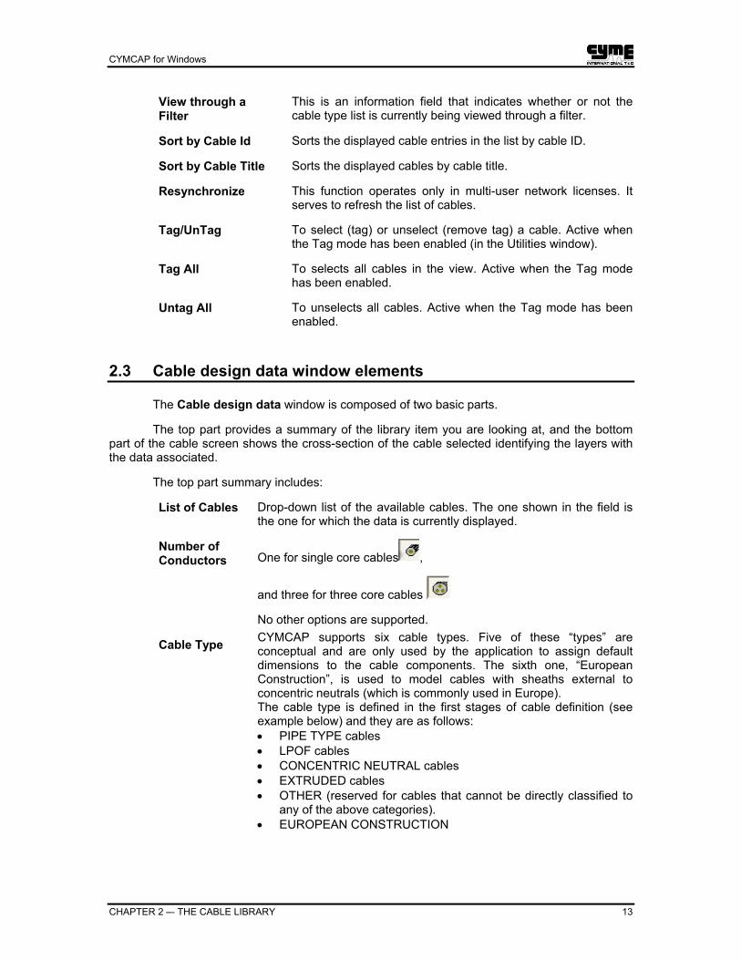
2.3 Cable design data window elements

The Cable design data window is composed of two basic parts.

The top part provides a summary of the library item you are looking at, and the bottom part of the cable screen shows the cross-section of the cable selected identifying the layers with the data associated.

The top part summary includes:

List of Cables Drop-down list of the available cables. The one shown in the field is the one for which the data is currently displayed.

Number of Conductors One for single core cables ,

and three for three core cables

No other options are supported.

Cable Type CYMCAP supports six cable types. Five of these “types” are conceptual and are only used by the application to assign default dimensions to the cable components. The sixth one, “European Construction”, is used to model cables with sheaths external to concentric neutrals (which is commonly used in Europe). The cable type is defined in the first stages of cable definition (see example below) and they are as follows: • PIPE TYPE cables • LPOF cables • CONCENTRIC NEUTRAL cables • EXTRUDED cables • OTHER (reserved for cables that cannot be directly classified to

any of the above categories). • EUROPEAN CONSTRUCTION

CYMCAP for Windows


Speed Bar A speed bar appears below the summary of the cable displayed. It lists the components available for the type of cable selected; and

indicates which component are currently used with a . When you click on the speed bar buttons, you toggle between Yes and No to display and hide the layer in question. When you enable a component for which the database does not contain associated data, the list of layers in the bottom part of the window will show you where data needs to be entered with red ellipses, or with the word “unknown”. When a component is not available for the type of cable selected, the

speed button for that layer will show a lock .

Notes: • There is no provision for default dimension assignment to the

cable type “OTHER” or “EUROPEAN CONSTRUCTION”. • There are no components availability restrictions for the cable type

“OTHER”. Note that such restrictions do apply to the remaining types.

• No pipe type cable can be modeled under the OTHER construction.

• The component availability restrictions are seen in the data entry dialog boxes as “locks” not allowing the user to select a particular component construction depending on the remaining data entered so far. These restrictions are not meant to be rigid and they simply reflect one philosophy of manufacturing practice from the very many available.

• In the EUROPEAN CONSTRUCTION type the Sheath/Sheath Reinforcement layers appear outside the Concentric Neutral layer on the layers speed bar.

This button gives access to the Short Circuit Ratings (/SCR) add-on module of CYMCAP.

CYMCAP for Windows


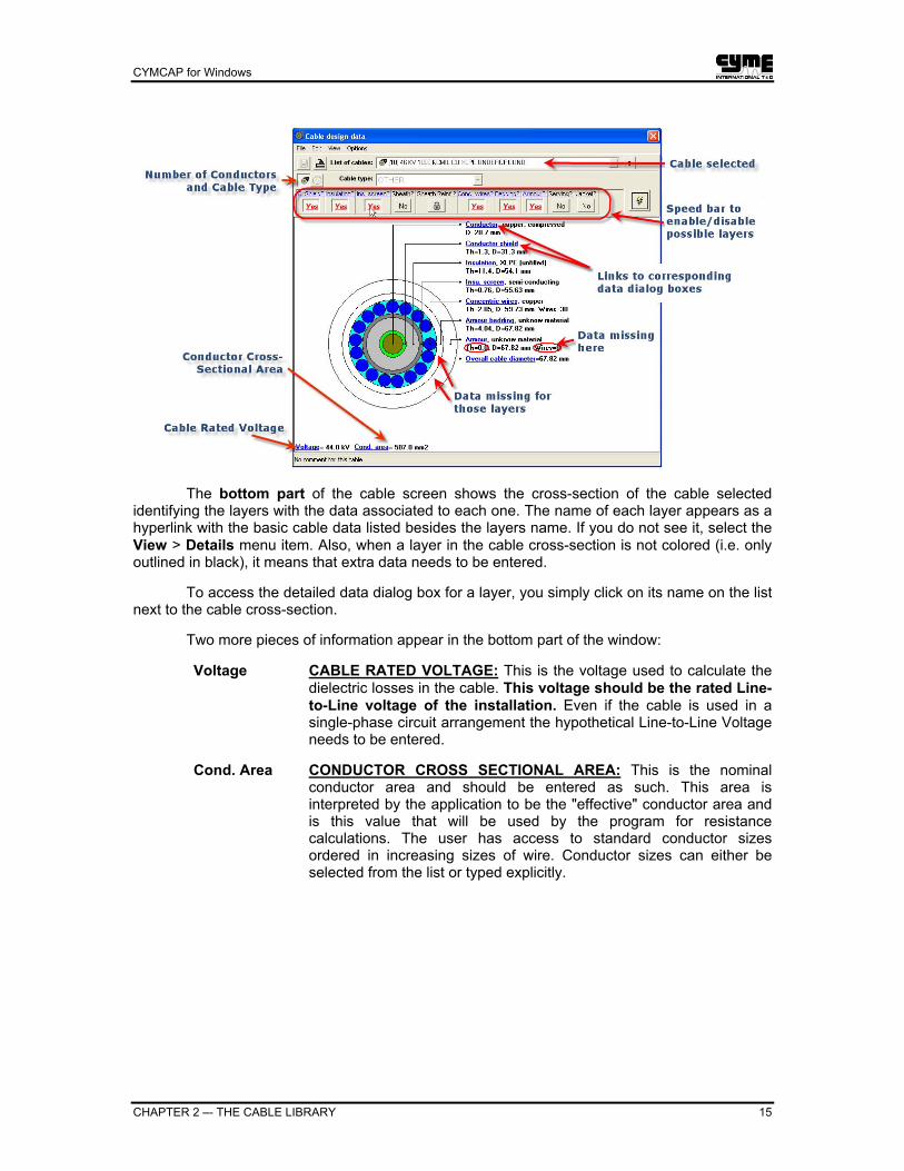
The bottom part of the cable screen shows the cross-section of the cable selected identifying the layers with the data associated to each one. The name of each layer appears as a hyperlink with the basic cable data listed besides the layers name. If you do not see it, select the View > Details menu item. Also, when a layer in the cable cross-section is not colored (i.e. only outlined in black), it means that extra data needs to be entered.

To access the detailed data dialog box for a layer, you simply click on its name on the list next to the cable cross-section.

Two more pieces of information appear in the bottom part of the window:

Voltage CABLE RATED VOLTAGE: This is the voltage used to calculate the dielectric losses in the cable. This voltage should be the rated Line-to-Line voltage of the installation. Even if the cable is used in a single-phase circuit arrangement the hypothetical Line-to-Line Voltage needs to be entered.

Cond. Area CONDUCTOR CROSS SECTIONAL AREA: This is the nominal conductor area and should be entered as such. This area is interpreted by the application to be the "effective" conductor area and is this value that will be used by the program for resistance calculations. The user has access to standard conductor sizes ordered in increasing sizes of wire. Conductor sizes can either be selected from the list or typed explicitly.

CYMCAP for Windows


2.4 Steps to create a new cable

The necessary steps to create a new cable and add it to the cable library are summarized below. An example applying those steps is the subject of section 2.6 Creating a new cable - Example

Step 1: Identify the layers and cable components and decide how they are to be modeled, according to the component availability CYMCAP offers. The component availability is listed starting at section 2.5 Cable components, materials and construction.

Step 2: Identify the cable components and define the materials they are made of. In case the program does not support a material for a given component, make certain that the necessary constants are available so that you can enter it as “custom”.

Step 3: Identify the cable components dimensions and make certain that every layer thickness is well identified. CYMCAP relies on layer thickness to conjecture equivalent layer diameters for both single core and three-core cables of all constructions. Furthermore, make certain that accurate data concerning length of lay for concentric wires armour and tapes are also available. These data are important to correctly estimate loss factors in 2-point bonded systems. It is always useful to ascertain that the cable construction dimensions are available from the manufacturer. The more the cable construction details are known, the less one has to rely on the default dimensions provided by the program.

Step 4: Select the system of Units for the session. Both Imperial and Metric systems are supported by CYMCAP. The cable dimensions can be entered in either inches (Imperial system) or mm (Metric). Once the cable dimensions are entered in any system they can be visualized in the other system by simply switching the Unit

system by clicking on the or icon.

Step 5: Enter the cable components and dimensions for the cable (see 2.5 Cable components, materials and construction).

Step 6: SAVE the newly entered cable data. Menu command File > Save or File > Save

As. You can also save by clicking on .

Step 7: Display a new listing of the library of cables in the Navigator (F3) and make sure that the newly entered cable appears on the list.

CYMCAP for Windows


2.5 Cable components, materials and construction When a cable is entered in the library, the user has considerable flexibility in specifying

both the available cable components as well as the materials these components are made of. In the paragraphs that follow, the cable components supported are outlined along with the parameters the program will use internally as a function of the component construction. Parameters and/or constants used by the application follow the ones in IEC-287-1-1/1994.

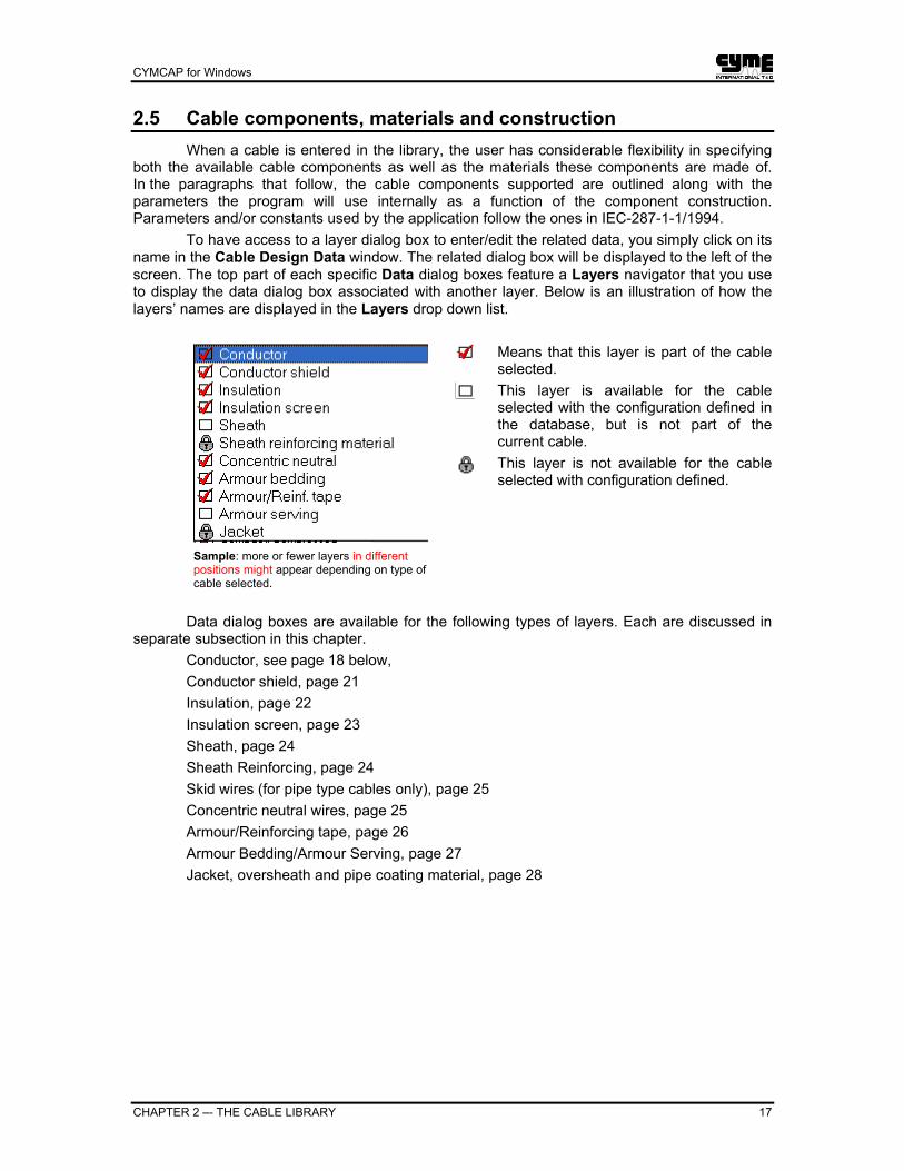
To have access to a layer dialog box to enter/edit the related data, you simply click on its name in the Cable Design Data window. The related dialog box will be displayed to the left of the screen. The top part of each specific Data dialog boxes feature a Layers navigator that you use to display the data dialog box associated with another layer. Below is an illustration of how the layers’ names are displayed in the Layers drop down list.

Means that this layer is part of the cable selected.

This layer is available for the cable selected with the configuration defined in the database, but is not part of the current cable.

Sample: more or fewer layers in different positions might appear depending on type of cable selected.

This layer is not available for the cable selected with configuration defined.

Data dialog boxes are available for the following types of layers. Each are discussed in

separate subsection in this chapter. Conductor, see page 18 below, Conductor shield, page 21 Insulation, page 22 Insulation screen, page 23 Sheath, page 24 Sheath Reinforcing, page 24 Skid wires (for pipe type cables only), page 25 Concentric neutral wires, page 25 Armour/Reinforcing tape, page 26 Armour Bedding/Armour Serving, page 27 Jacket, oversheath and pipe coating material, page 28

CYMCAP for Windows


A number of commands are common to all Data dialog boxes. You will find them at the bottom of the windows:

Previous Displays the previous layer on the list. Next Displays the next layer on the list. Reset Erases all changes made during the current editing session. Ok Retains the information entered in the window, displays the data on the

cross-sectional display and closes the window. Cancel Closes the data window without retaining the information entered in that

window from the moment it was last displayed. Clicking the X at the right hand top corner has the same effect.

2.5.1 Conductor data

CYMCAP for Windows


2.5.1.1 Conductor material

The conductor material can be copper, aluminum or any other “custom” material. Independently of the choice, the program needs the DC conductor material resistivity at 20 °C (in Ω-m) and the temperature coefficient for the resistance (/°K at 20°C). When aluminum or copper is selected the program assumes the following values:

Copper ρ=1.7241e-08, α=3.93e-03

Aluminum ρ=2.8264e-08, α=4.03e-03

When the user selects the conductor material, these values must be provided.

Resistance values per IEC 228 The resistance of the conductors can be calculated or taken from the tabulated values in the Standard IEC 228. The conductor material, type and construction are all taken into account during the course of the calculations. The user may choose the option to obtain the resistance of the conductor from the resistance tables of the Standard IEC 228. Depending on conductor cross-sectional area, construction type and material, a different resistance value will be considered. The following restrictions and/or assumptions apply:

• IEC-228 resistance values apply ONLY to copper and aluminum conductors.

• IEC-228 resistance values pertaining to PLAIN conductors are considered. In other words, the current version of the program does not support METAL-COATED conductors.

• For conductor sizes in-between standard tabulated values, linear Interpolation is used to arrive at the estimated resistance value.

• If the user wishes to consider resistances applicable to class 1-conductors (table I of IEC 228), the choice "solid" must be used for the Conductor construction option.

• If the user wishes to consider resistances applicable to class 2 conductors (table II of IEC 228), the choices "stranded", "compact/compressed", "sector-shaped" and "oval" are pertinent. No other conductor construction option is supported for IEC-228 compatible calculations.

• If a conductor cross-section is entered for the cable and not supported by IEC 228, the program will revert to the alternate mode, i.e. the resistance will be calculated.

• For conductor cross-sections, corresponding to blank entries in the tables 1 and 2 of IEC 228, the program will revert to the alternate mode, i.e. the resistance will be calculated.

2.5.1.2 Conductor construction

The following choices for conductor construction are supported:

• Stranded (round)

• Compact or compressed (round)

• 4 segments

• Hollow core

• 6 segments

• Sector shaped

• Oval

CYMCAP for Windows


• Solid

• Segmental

• Segmental peripheral-strands

The selections available are contingent upon the cable type selected as well as the conductor dimensions. The program will indicate which options are valid by highlighting them in the Construction selection menu of the Conductor data dialog box.

Means the option selected.

Means that the option is available for selection.

Means that the option is not available for the cable selected .

2.5.1.3 Drying and Impregnation

This information is used to properly correct for skin and proximity effects when calculating the conductor resistance.

Skin and proximity effect loss factors Skin and proximity effects are used to calculate the ac resistance of the conductor by adjusting the dc conductor resistance by the factors Ys (skin effect) and Yp (proximity effect) as follows:

Rac = Rdc (1 + Ys +Yp): Rac, Rdc are AC and DC resistances, respectively. In calculating Ys and Yp the constants Ks and Kp are used. The program assumes the following values based on conductor construction. Note that these values have been compiled for copper conductors. Nevertheless, the same values will be assumed for aluminum except for segmented conductors which value is shown in the table. The approximation is considered to be on the safe side.

Conductor Construction Ks Kp Round stranded dried and impregnated 1.00 0.80 Round stranded not dried and impregnated 1.00 1.00 Round compact dried and impregnated 1.00 0.80 Round compact not dried and impregnated 1.00 1.00 Round segmental (Copper 4 segments) 0.435 0.37 Round segmental (Copper 6 segments) 0.39 0.37 Hollow, helical stranded, dried, impregnated * 0.80 Sector shaped dried and impregnated 1.00 0.80 Sector shaped not dried and impregnated 1.00 1.00 Round segmental (Aluminum 4 segments) 0.28 0.37 Round segmental (Aluminum 5 segments) 0.19 0.37 Round segmental (Aluminum 6 segments) 0.12 0.37

* See calculation method in table 2 of the IEC Standard 287-1-1 The user can also enter different values using the CYMCAP GUI as shown in the following figure.

CYMCAP for Windows


2.5.2 Conductor shield data

The program supports "conductor screens", as a cable component The term "shield" is often used as equivalent to the term "screen".

Notes:

• Non-metallic screens are modeled as part of the insulation.

• If a conductor shield is modeled, the program will assume its material to be the same as the insulation material.

• The conductor shield is taken into account as part of the insulation when the thermal resistance is computed, but it will not be considered as part of the insulation for the calculation of the dielectric losses.

CYMCAP for Windows


2.5.3 Insulation data

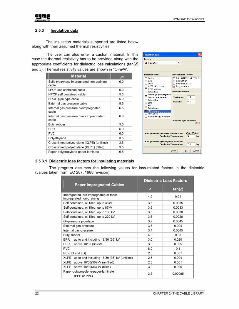
The insulation materials supported are listed below along with their assumed thermal resistivities.

The user can also enter a custom material. In this case the thermal resistivity has to be provided along with the appropriate coefficients for dielectric loss calculations (tan(δ) and ε). Thermal resistivity values are shown in °C-m/W.

Material ρi

Solid type/mass impregnated non draining cable

6.0

LPOF self contained cable 5.0 HPOF self contained cable 5.0 HPOF pipe type cable 5.0 External gas pressure cable 5.5 Internal gas pressure preimpregnated cable

6.5

Internal gas pressure mass impregnated cable

6.0

Butyl rubber 5.0 EPR 5.0 PVC 6.0 Polyethylene 3.5 Cross linked polyethylene (XLPE) (unfilled) 3.5 Cross linked polyethylene (XLPE) (filled) 3.5 Paper-polypropylene-paper-laminate 6.5

2.5.3.1 Dielectric loss factors for insulating materials

The program assumes the following values for loss-related factors in the dielectric (values taken from IEC 287, 1988 revision).

Dielectric Loss Factors Paper Impregnated Cables

ε tan(δ) Impregnated, pre-impregnated or mass-impregnated non-draining 4.0 0.01

Self-contained, oil filled, up to 36kV 3.6 0.0035 Self-contained, oil filled, up to 87kV 3.6 0.0033 Self-contained, oil filled, up to 160 kV 3.6 0.0030 Self-contained, oil filled, up to 220 kV 3.6 0.0028 Oil-pressure pipe-type 3.7 0.0045 External gas-pressure 3.6 0.004 Internal gas-pressure 3.4 0.0045 Butyl rubber 4.0 0.05 EPR up to and including 18/30 (36) kV 3.0 0.020 EPR above 18/30 (36) kV 3.0 0.005 PVC 8.0 0.1 PE (HD and LD) 2.3 0.001 XLPE up to and including 18/30 (36) kV (unfilled) 2.5 0.004 XLPE above 18/30(36) kV (unfilled) 2.5 0.001 XLPE above 18/30(36) kV (filled) 3.0 0.005 Paper-polypropylene-paper-laminate (PPP or PPL)

3.5 0.00095

CYMCAP for Windows


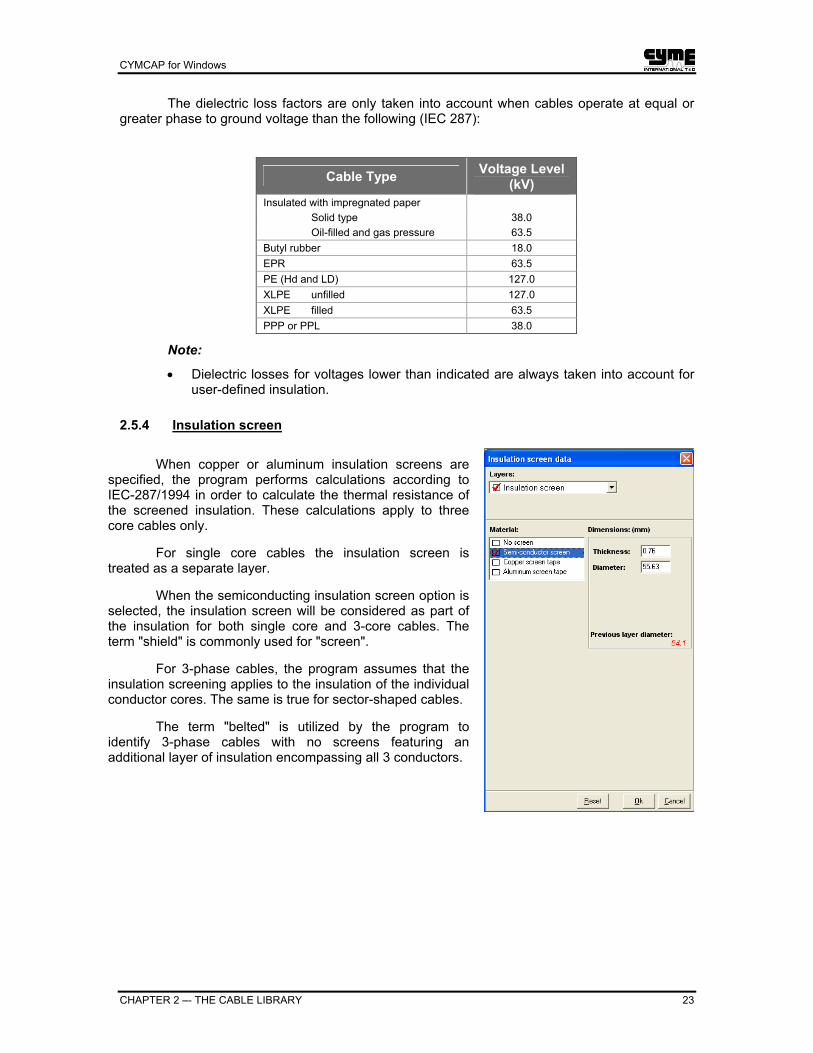
The dielectric loss factors are only taken into account when cables operate at equal or greater phase to ground voltage than the following (IEC 287):

Cable Type Voltage Level (kV)

Insulated with impregnated paper Solid type 38.0 Oil-filled and gas pressure 63.5 Butyl rubber 18.0 EPR 63.5 PE (Hd and LD) 127.0 XLPE unfilled 127.0 XLPE filled 63.5 PPP or PPL 38.0

Note:

• Dielectric losses for voltages lower than indicated are always taken into account for user-defined insulation.

2.5.4 Insulation screen

When copper or aluminum insulation screens are specified, the program performs calculations according to IEC-287/1994 in order to calculate the thermal resistance of the screened insulation. These calculations apply to three core cables only.

For single core cables the insulation screen is treated as a separate layer.

When the semiconducting insulation screen option is selected, the insulation screen will be considered as part of the insulation for both single core and 3-core cables. The term "shield" is commonly used for "screen".

For 3-phase cables, the program assumes that the insulation screening applies to the insulation of the individual conductor cores. The same is true for sector-shaped cables.

The term "belted" is utilized by the program to identify 3-phase cables with no screens featuring an additional layer of insulation encompassing all 3 conductors.

CYMCAP for Windows


2.5.5 Sheath

Sheath material and resistivity

The sheath electrical resistivity ρ (Ω-m at 20°C) and the thermal coefficient α (1/°C) are required for the calculations. Supported materials read as follows:

Material ρ α

Lead 21.4e-08 4.0e-03 Aluminum 2.84e-08 4.03e-03 Copper 1.72e-08 3.93e-03

The user can enter any other material by selecting “Custom” in the Material list, but in this case the values of ρ and α must be entered; the program will display a dialog box to allow the user to do so.

Sheath construction

The program supports both radial and longitudinal construction for sheath corrugation for the case of aluminum, copper and custom only. When default dimensions are set by the program, the calculation for the sheath thickness followed for the case of aluminum, is applied to copper and custom; see section 11.6 Sheath related defaults.

2.5.6 Sheath Reinforcing Material

CYMCAP allows the user to enter a sheath reinforcement tape for sheathed cables or tape over insulation screen for pipe type cables. The thickness refers to the radial dimension and it is used to compute the diameter and vice versa. Width is the axial dimension of the tapes as shown in the illustration below.

The length of lay is the longitudinal distance required for a particular tape to give one revolution around the previous layer (see the figure below). When the length of lay is not available, a value of 10 times the previous layer diameter can be used.

CYMCAP for Windows


2.5.7 Skid wires (for pipe type cables only)

Skid wires are applicable to pipe type cables only. Despite the fact that skid and concentric wires share similar information, skid wires data entry dialog boxes are dedicated to pipe type cables. No cable can have both skid and concentric neutral wires. The program assumes that the skid wires are semicircles. Two skid wires will be assumed present, by default, by the program but the number can be changed; see section 11.5 item 5. Skid Wires. Length of lay considerations applicable to skid wires, are identical to the ones for concentric neutral wires.

2.5.8 Concentric neutral wires

Concentric neutral wires are, usually, return wires in distribution cables. The program assumes that these wires are bare (no insulating or plastic wrap that they may be equipped with, is supported). Data for the concentric neutral comprise the wire size, the number of wires as well as the length of lay; see section 11.2 Concentric neutral cables for defaults. The concentric wires may be made of copper, brass, zinc, or stainless steel. CYMCAP supports flat-straps concentric neutrals.

Material ρ α Copper 1.7241e-08 3.93e-03 Aluminum 2.8264e-08 4.03e-03 Stainless steel 70.000e-08 0.000000 Zinc 6.1100e-08 0.004 Brass/Bronze 3.5000e-08 0.003

If other than the above materials are to be used (select “Custom” to do so), the user has to provide resistivity and temperature coefficient. ρ is expressed in Ω-m at 20 °C and α in 1/°C.

CYMCAP for Windows


2.5.9 Armour/Reinforcing tape

CYMCAP supports cable armour assemblies in the form of either wires or tapes.

For the case of armour wires, the program requests as data the number of wires (if not touching), the wire size and the length of lay. For the case of armour tapes, besides the number of tapes and the length of lay, the tape width must also be provided.

For thermal calculations the armour resistivity as well as the thermal coefficients are also needed

The following materials are internally supported: (ρA is expressed in Ω-m at 20°C and α in 1/°C).

Material ρA α Custom non magnetic tape User-defined User-defined Custom, magnetic armour wires User-defined User-defined Custom magnetic tape User-defined User-defined Custom, non magnetic wires User-defined User-defined Steel wires touching 13.8 E-08 0.0045 Steel wires not touching 13.8 E-08 0.0045 Steel tape reinforcement 13.8 E-08 0.00393 Copper armour wires 1.721 E-08 0.00393 Stainless steel armour 70.0 E-08 0.0 IEC TECK armour 2.84 E-08 0.0043

If any other material is to be used (select “Custom” to do so), the user has to supply the above parameters.

When magnetic losses are of importance, additional data needs to be entered to model the eddy currents and hysterysis losses of the armour. The parameters needed are the longitudinal and transverse permeability (AME and AMT respectively) as well as the angular time delay γ. The user can enter these parameters or have the program select them. When the program selects, it will assume:

• AME=400, AMT=10 for steel wires touching or

• AMT=1 for steel wires not touching and GAMMA=45 degrees.

The same values will be assumed for steel tapes. Magnetic properties modelling for the armour is supported only for steel armour assemblies.

CYMCAP for Windows


2.5.10 Armour Bedding/Armour Serving

CYMCAP defines as armour bedding the layer that is normally encountered below the armour assembly. Armour serving is defined as the layer of protective coverings sometimes found above the armour assembly. The following materials are supported for armour bedding.

Material Thermal resistivity (°C-m/W)

Compounded jute and fibrous materials

ρ=6.00

Rubber sandwich ρ=6.00

If any other material is to be used, the user must provide the thermal resistivity. Values for many insulating materials are given in section 2.5.3 Insulation data.

CYMCAP for Windows


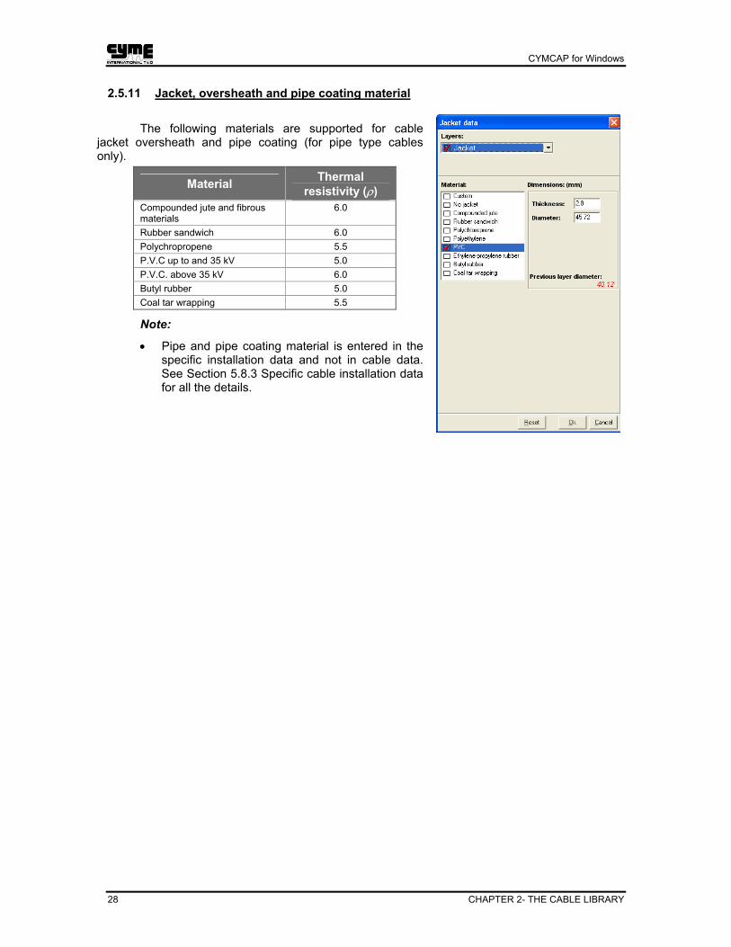
2.5.11 Jacket, oversheath and pipe coating material

The following materials are supported for cable jacket oversheath and pipe coating (for pipe type cables only).

Material Thermal resistivity (ρ)

Compounded jute and fibrous materials

6.0

Rubber sandwich 6.0 Polychropropene 5.5 P.V.C up to and 35 kV 5.0 P.V.C. above 35 kV 6.0 Butyl rubber 5.0 Coal tar wrapping 5.5

Note:

• Pipe and pipe coating material is entered in the specific installation data and not in cable data. See Section 5.8.3 Specific cable installation data for all the details.

CYMCAP for Windows


2.6 Creating a new cable - Example

In this section, we will go through the stages of creating a new cable for illustration purposes. The cable will be a typical 250KCMIL distribution cable, rated 35 kV. The cable features Aluminum stranded conductor, XLPE insulation and copper concentric neutral wires. In what follows a typical sequence of the steps/screens/dialog boxes required to enter a cable is outlined.

To create a new cable in the library, position the highlight bar on any cable and click on the New button. If the existing cable is to be used as a template for your new one, answer “Yes” to the ensuing prompt. In our current example, No existing cable is used as a template. Then, the following screen indicates that it is required to enter a cable ID and a cable Title.

The cable ID should be unique because it is used internally as a database index. It is the cable ID and the cable title that appear in the cable type library browser. Comments are optional, but frequently important.

Click OK to accept the data entered and the screen that follows allows the user to begin defining in details the cable construction, from the point of view of component availability.

First specify whether the new cable will be a single-core or a three-core, by clicking on one of the buttons next to the Cable Type combo box:

To specify a single-conductor cable.

To specify a three-conductor cable

Then specify the cable type as EXTRUDED in the Cable type combo box.

CYMCAP for Windows


The program then prompts for the nominal cable voltage (kV); indicate “35” kV, then the click OK button.

The next piece of data required is the conductor size. Open the standard conductor sizes scroll list and select “250 KCMIL”. A default Conductor Area will then be displayed, you may change this.

Once the conductor size and the voltage are entered, the program is ready to accept more instructions by displaying the following screen. You will notice that the Speed Bar now displays the layers that are possible to be added based on the information entered up to this point.

CYMCAP for Windows


It is seen that no dimensions are entered at all, as the encircled quantities show. The program also indicates that no materials were defined at all. Before proceeding to materials and dimensions, we must first specify the generic cable components. Among the generic components only the cable insulation has been enabled so far (see the Speed Bar). Let us enable the insulation screen, the concentric neutral and the jacket.

Note that the concentric wires were not drawn yet. They will be displayed on the cross-section when specific data is entered later.

CYMCAP for Windows


Once all the generic components for the cables are entered, we tell the program that their definition has ended by clicking on the Complete Cable button appearing on the top part of the window. The program then displays the Data dialog box for the first generic component, the conductor, in order to accept further instructions about materials, construction type and dimensions. Clicking on the Reset button will display the last saved data. Note that the program will allow saving only once all the data required defining all the layers of your cable will be entered.

Several alternatives for the conductor material and construction are available. Choices that are either not permitted or irrelevant, based on the data entered so far, are locked, as the appropriate locker symbol next to them indicates, and are not available for selection.

Define the material, construction and dimensions on the same screen and to proceed to the following generic component, click the Next button at the bottom of the Conductor Data dialog box. You will notice that when you click Next, the layers list in the cross-section window will now display the information you have just entered. Clicking OK has the same effect on the cross-section, but it will close the Data dialog box.

CYMCAP for Windows


The next layer of our example is the insulation. The dialog box for the insulation is as follows:

The information that needs to be entered here includes the maximum design (steady

state) and emergency (transient) operating temperatures the particular cable can withstand. Default values are assigned automatically depending on the insulation type material selected by the user. The program will use these values for the corresponding analysis options unless changed by the user.

You proceed in this fashion for the remaining layers. Missing data is indicated with a red circle or with the word “unknown” on the cross-section display. Once all the necessary data is

entered, the Save button will be enabled, as well as the corresponding File > Save and the File > Save as menu items.

Note that when you open a cable that is contained in the library, the Save button and the Save menu option are disabled until you make a change. When they are enabled and you use them, the program saves the data under the Cable ID and the Cable Title that are displayed.

The Save As menu option remains available even if you do not make a change to the cable displayed. If you use that last option, the program will prompt you to enter new Cable ID and Cable Title.

CYMCAP for Windows


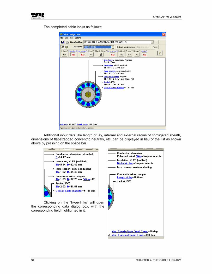
The completed cable looks as follows:

Additional input data like length of lay, internal and external radius of corrugated sheath, dimensions of flat-strapped concentric neutrals, etc, can be displayed in lieu of the list as shown above by pressing on the space bar.

Clicking on the “hyperlinks” will open the corresponding data dialog box, with the corresponding field highlighted in it.

CYMCAP for Windows


2.7 Useful considerations

2.7.1 Cable layers

a. The sequence of cable components in CYMCAP assumes a start from the conductor and expands outwards with the insulation, insulation shield, sheath, sheath reinforcement, concentric neutral wires, armour bedding, armour, armour serving, and finally the jacket. It is in this spirit that the terms are used in the program and their definition should be respected.

b. When creating a cable, it is possible that layers not directly identifiable with any of the available components are encountered. Closer inspection, often, reveals that one of the available layers by the program can be directly used because different names are often interchangeably used for the same layer. For example, CYMCAP will not accept a cable jacket once armour is defined for a given cable. The cable jacket then can alternatively be modeled as armour serving.

c. If the need for a layer not supported by CYMCAP arises, you can combine two layers in one by calculating an equivalent thermal resistivity for two layers in series. This can be particularly useful for the cases where materials of different thermal resistivity are used for either armour serving or bedding. A conservative approach from a thermal resistance point of view would be to model the two layers as one having as thermal resistivity the one with the higher value.

d. When a layer is deleted, the user does not have to reflect the change in the dimensions imposed beyond that layer towards the cable surface. The program will automatically adjust the dimensions accordingly. The same holds true if a layer is inserted. If a layer is deleted and then reinserted, the layer dimensions are automatically restored as long as the cable was not saved or that the program session has not been terminated.

2.7.2 Particular modeling

a. When cables with oval conductors are to be modeled, the user should enter the

equivalent round conductor diameterD D Dmajor or= min , where

Dmajor and D ormin are the corresponding lengths of the major and minor elliptical axis of the oval conductor.

e. Model metallic conductor screens as part of the conductor. Similarly, model semiconducting conductor screens as part of the insulation, include semiconductive swellings in the semiconductive screen over the insulation, etc.

f. To model armour wires imbedded in the jacket, you can represent the portion of the layer below the wires as armour bedding, the wires as armour, and the portion of the layer above the wires as armour serving.

g. Interjackets and jackets around armour assemblies, should be modeled as armour bedding and serving, because the program does not allow for jacket when armour is present.

h. Metallic parts that are associated with circulating currents should be modeled as sheaths, even if they are termed screens. This assures that the program calculates properly the loss factors.

CYMCAP for Windows


2.7.3 SL-type cables

SL-type cables are 3-conductor cables characterized by the fact that every core has its own sheath or armour wires. The program supports either options but not both simultaneously.

The SL-type construction is identified during the cable data entry by specifying either individual sheath or individual armour construction. Note that the following restrictions apply to the construction of SL-type cables:

• SL-type cables are not permitted to have metallic insulation screens.

• No sheath reinforcement is supported for SL-type cables.

• Corrugated sheaths are not supported for SL-type cables.

• SL-type cables will either have individual sheaths or individual concentric neutral wires but not both.

• When SL-type cables are modeled, the bonding arrangement selections available are either “single point bonded” or “two point bonded”.

• Default dimensions for SL-type cables sheaths and armour wires follow the same defaults as for single-core cables.

2.7.4 Custom materials and thermal capacitances

CYMCAP gives the user the possibility to enter custom materials for many of the cable components metallic or not. For many non-metallic parts as: insulation, armour bedding, serving etc. the thermal capacitance of the particular component is needed for transient ampacity calculations. Although the program will consider specific thermal capacitance values for known and tabulated selected material types, when custom materials are specified typical values are assumed for the thermal capacitances. The application supports ASCII fields for any type of user-defined components so that their name, as well as their parameters can be clearly identified. The following screen illustrates the concept.

CYMCAP for Windows


2.8 Filter Editor

It is not uncommon to desire to locate cables with particular construction characteristics, in addition to the major generic classification provided by the primary filter that is the Search Utility of the Navigator pop-up menu (see section 2.2.2 Cable library pop-up menu). In this case, invoking the more advanced search/filtering facilities of CYMCAP is needed. From the cable library navigator screen, invoke the Filter Editor as shown below:

Once the filter is invoked, the user is presented with the option to specify any particular cable characteristics for the search, as shown below.

In this particular example illustrated, single core, medium voltage cables (rated higher than 6.00 kV) featuring a conductor cross-section larger than 1250 mm2, copper conductor of stranded construction, with concentric neutral and XLPE insulation are specified for the search.

CYMCAP for Windows


Notes:

• More detailed searches comprising non-metallic components can also be included.

• To bring any cable component attribute in the Filter elements selected list and collect all the desired cable characteristics as search attributes, highlight the desired feature and bring it over by clicking on the right arrow.

• To remove a selection, highlight the selected attribute to the right and use the left arrow to remove it from the selection list.

• The specified search characteristics are summarized at the bottom of the screen in the Filter to apply on Cable Library field.

• A name can be given to the particular filter search characteristics set and saved for future reference.

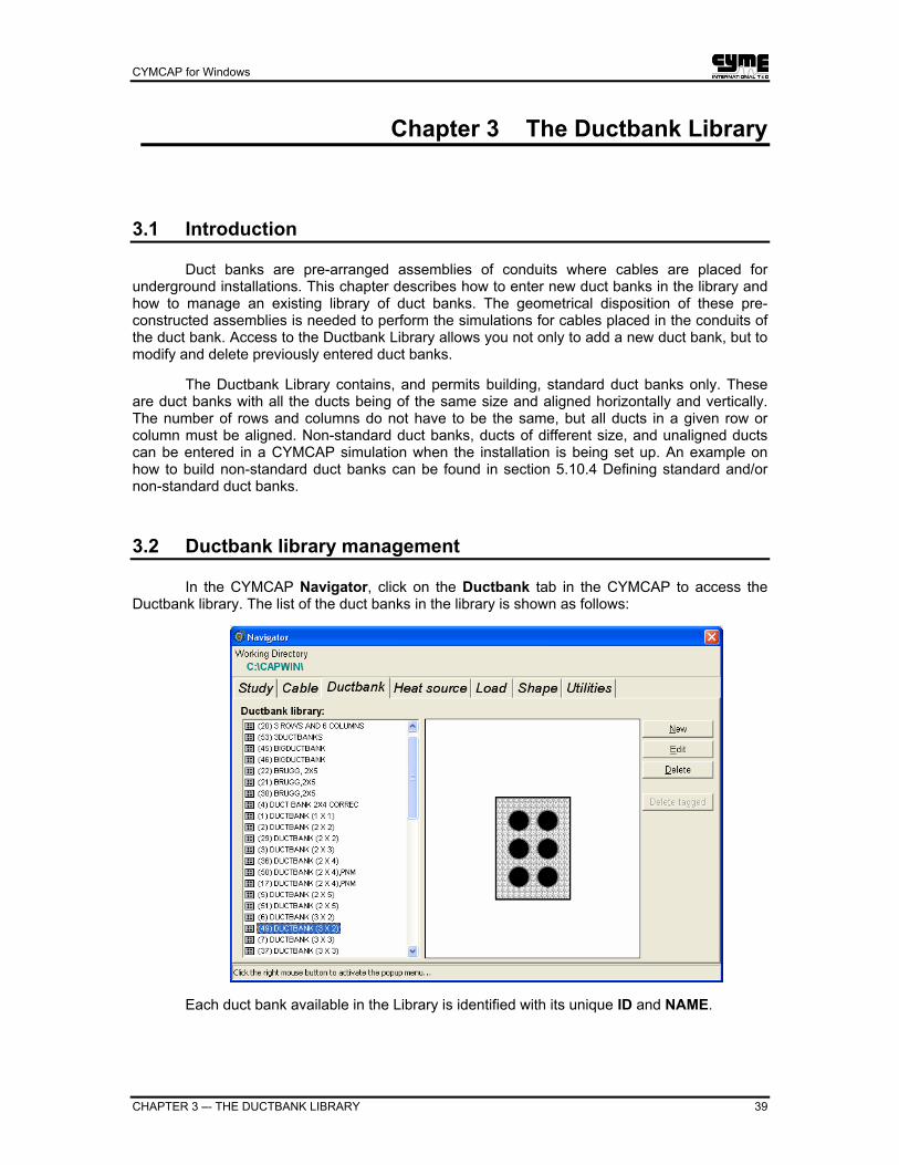
CYMCAP for Windows

CHAPTER 3 –- THE DUCTBANK LIBRARY 39

Chapter 3 The Ductbank Library

3.1 Introduction

Duct banks are pre-arranged assemblies of conduits where cables are placed for underground installations. This chapter describes how to enter new duct banks in the library and how to manage an existing library of duct banks. The geometrical disposition of these pre-constructed assemblies is needed to perform the simulations for cables placed in the conduits of the duct bank. Access to the Ductbank Library allows you not only to add a new duct bank, but to modify and delete previously entered duct banks.

The Ductbank Library contains, and permits building, standard duct banks only. These are duct banks with all the ducts being of the same size and aligned horizontally and vertically. The number of rows and columns do not have to be the same, but all ducts in a given row or column must be aligned. Non-standard duct banks, ducts of different size, and unaligned ducts can be entered in a CYMCAP simulation when the installation is being set up. An example on how to build non-standard duct banks can be found in section 5.10.4 Defining standard and/or non-standard duct banks.

3.2 Ductbank library management

In the CYMCAP Navigator, click on the Ductbank tab in the CYMCAP to access the Ductbank library. The list of the duct banks in the library is shown as follows:

Each duct bank available in the Library is identified with its unique ID and NAME.

CYMCAP for Windows

40 CHAPTER 3–- THE DUCTBANK LIBRARY

A picture showing the duct bank cross section is displayed in the viewer pane to the right of the window for the corresponding duct bank in the list when the highlight bar is positioned on the name. Press the Up and Down arrow keyboard keys to browse through the library. CYMCAP allows the user to view the salient aspects of the various duct banks without resorting to detailed editing.

To ADD a duct bank to the library, highlight any library entry and click the New button located to the right of the Navigator list. You will be prompted with the option to either use a duct bank as a template or create a completely new one. If you choose the template option, the entry the highlight bar is on will be used as the template.

To MODIFY a duct bank highlight the duct bank of interest and left-click with the mouse on the Edit button located to the right of the Navigator list. The same task can be accomplished by positioning the highlight bar on the entry of interest and double-clicking on the left mouse button.

To DELETE a duct bank you position the highlight bar on it and left-click with the mouse on the Delete button located to the right of the navigator list. You can also click and drag any entry from the library to the disposal bin shown in the upper right corner of the navigator window.

3.2.1 Creating a new duct bank. An illustrative example.

A new duct bank will be created for illustration purposes. The duct bank will be a sample 3x3 duct bank, i.e. consisting of 3 series of conduits and 3 columns of conduits. In what follows, a typical sequence of the steps/screens/dialog boxes required to enter a new duct bank is outlined for illustration purposes.

To create a new duct bank in the library, position the highlight bar on any entry and click on the New button. If the existing duct bank is to be used as a template for the new one, answer Yes to the ensuing prompt.

For this example, we will not use an existing duct bank as a template.

The program then prompts for the entry of a Duckbank name.

CYMCAP for Windows

CHAPTER 3 –- THE DUCTBANK LIBRARY 41

Once the duct bank name is entered, two windows are displayed side by side: the Ductbank Library designer dialog box and the Ductbank design data window. The geometrical details outlining the duct bank construction are entered in the Ductbank Library designer dialog box. The cross-section of the duct bank is shown in the Ductbank design data window is updated as the data characteristics are entered in the Ductbank Library designer dialog box.

When the cursor is positioned into any data entry field, the dimension in question is outlined on the small auxiliary help screen appearing in the Ductbank Library designer dialog box.

CYMCAP for Windows

42 CHAPTER 3–- THE DUCTBANK LIBRARY

The following illustrates the new duct bank with its complete characteristics.

Click OK to accept the data entered and save the new duct bank in the library. The newly entered duct bank now appears as a new entry in the Ductbank Library.

CYMCAP for Windows

CHAPTER 4 –- LOAD CURVES/HEAT SOURCE CURVES AND SHAPE LIBRARY 43

Chapter 4 Load-Curves/Heat Source Curves and Shape Libraries

4.1 Introduction

This chapter describes how to manage the last three libraries of CYMCAP. In what follows, the terms “Load curve” and “Heat source curve” are treated as conceptually identical, as far as library management is concerned, despite their physical difference. The term “Curve”, wherever used, means both. Whatever statements are made, however, for Load curves, apply equally well to Heat Source curves. These curves are used by CYMCAP only for TRANSIENT ANALYSIS.

Load Library – This library includes the available load curves, which are the patterns of current versus time, and that are used to indicate how the current in a given cable varies as a function of time over a specific time period. Access to a wide variety of loading patterns is thus assured for various transient studies. Much like the various types of cables, the different load curves are kept in a separate library. You can think of a Load Curve as being the weekly load profile of a particular feeder section.

Heat Source Library – This library contains the Heat Source curves, which are the patterns of heat source intensity versus time, and that are used to indicate how the heat source intensity varies as a function of time over a specific time period.

The Shape Library contains the shapes that are the building blocks used to construct both the Load curves and the Heat Source curves. The Shape library is common to both the Load Library and the Heat Source Library. A shape can be related to the daily load profile of a particular feeder section.

4.1.1 Curves and Shapes

CYMCAP uses the notion of Shapes to assure through modularity flexibility and efficiency in describing the various curve variations versus time.

A Shape is essentially a curve that spans at most 24 hours. Shapes are used to represent daily variations and feature, typically, hourly resolution. They need, however, to last at least 10 minutes since the numerical techniques of the CYMCAP engine do not have the resolution to properly compute shorter variations. The various shapes can be stored separately in the Shape Library. This shape library can be accessed when constructing a curve that spans one or more days. It is useful therefore to conceptualize the shapes not as stand-alone short-term Load variations but as the building blocks for the Load curves.

A load curve describes the variation of the Loading of Cable/Heat Source intensity with time. It may be composed of one or more shapes, depending on the duration of the transient to be simulated. Curves can span time intervals ranging from a fraction of a day to one week.

It is important to realize that CYMCAP forms an association between shapes and curves. No curve can be defined without a shape, and at least one shape is necessary to construct a curve. When shapes are modified within the shape library, these actions directly affect the curves associated with these shapes. No shape that belongs to an existing curve can be deleted.

CYMCAP for Windows

44 CHAPTER 4 –- LOAD CURVES/HEAT SOURCE CURVES AND SHAPE LIBRARY

N.B.: All variations, within the context of the curve definition, are expressed in p.u. The base quantity is the current/heat source intensity the cable/heat source carries at steady state as resulted/defined from the steady state ampacity or temperature simulations.

CYMCAP is also capable of interpreting recorded field measurements and construct Load Curves that faithfully reproduce these recordings, with an hourly resolution. These measurements need to be logged in an ASCII file that follows a specific FORMAT. The resulting Load curves are directly usable by the program for transient studies.

4.2 Shape Library management

The main tool for managing the Shape Library is the CYMCAP Navigator. Clicking on the Shape tab of the Navigator gives access to the Shape Library. The list of all available shapes in the shape library appears as shown in the following illustration:

The Shape Library is equipped with a browser that is shape-sensitive. Whenever the highlight bar is positioned on a particular shape, the lower part of the window shows that shape. This way, CYMCAP allows rapid visualization of the shapes without resorting to detailed editing.

To EDIT a shape, position the highlight bar on the shape to be edited and click on the Edit button to the right. You can also edit a shape by double-clicking on it with the left mouse button.

To CREATE a new shape, position the highlight bar on any shape and click on the New button to the right. The program will ask if you want to use the shape which name is highlighted in the list as a template or if you want to create a brand new one.

To RENAME a shape you must Edit it first.

CYMCAP for Windows


To DELETE a shape, position the highlight bar on the shape to be deleted and click on the Delete button to the right. If that shape is used within a Load curve a warning will follow.

4.2.1 Creating a new shape – An Illustrative example

Assume a shape that spans 24 hours, with the following characteristics:

• The first 2 hours will experience a load current of 0.3 p.u.,

• the next 4 hours a load current of 0.6 p.u.,

• the next 5 hours a load current of 0.85 p.u.,

• the next half hour a load current of 0.34 p.u.,

• the next 4 hours a current of 0.7 p.u.,

• the next 5 hours a current of 0.5 p.u.

• and the remaining 3.5 hours a current of 0.92 p.u.

Enter the CYMCAP Navigator and access the Shape Library. Position the highlight bar on any shape and click on New. In the screen that follows, the prompt demands if the current shape is to be used as a template. We will create a new shape from scratch, thus the answer to the prompt is No.

We next enter the Shape manager workbench. It is at this point that data particular to

this shape can be entered. At first a title is needed for the shape. This title must be unique and different from the remaining shape titles.

CYMCAP for Windows


After entering the title, the time-current data need to be entered. Note that when the table first appears, all entries of the table are blank and there is no drawing for any segments of the shape. As soon as data is entered for the shape, the drawn curve is refreshed in correspondence.

Notes:

• When data for a shape is entered, the current value cannot exceed 1.0 p.u. Scaling factors can, however, be used when building the Load Curve.

• Every time the cursor is positioned in a given field, the appropriate part of the drawing is highlighted for better visualization.

• Also, you have access to the complete list of shapes through the list of shapes accessible at the top. Note that this list is accessible only when the shape that is displayed has been saved.

The Shape Manager workbench features six command buttons at the top of the window. They are all used for shape management purposes. Position the cursor on any of the buttons and a tool-tip appears indicating their function. More specifically:

CYMCAP for Windows


Saves the shape with the modifications.

Saves as a new shape.

Delete the shape.

Inquires what load curve(s) utilizes that shape.

Pust a shape in the windows clipboard.

Reverts to the original entries defining a shape, once a modification was effected.

4.2.2 Shifting a shape – An illustrative example

Shapes normally start at “time 0”. You may need, however, to shift a shape so that any given time can be considered its origin. This is particular useful when you want the origin of your transient study to coincide with the steady state calculation. The application permits this operation to be done without redefining the shape using the Shift curve… button located at the bottom of the window. For instance, assume that the following shape is to be shifted at the 5th hour. Click on Shift curve… and enter the desired hour.

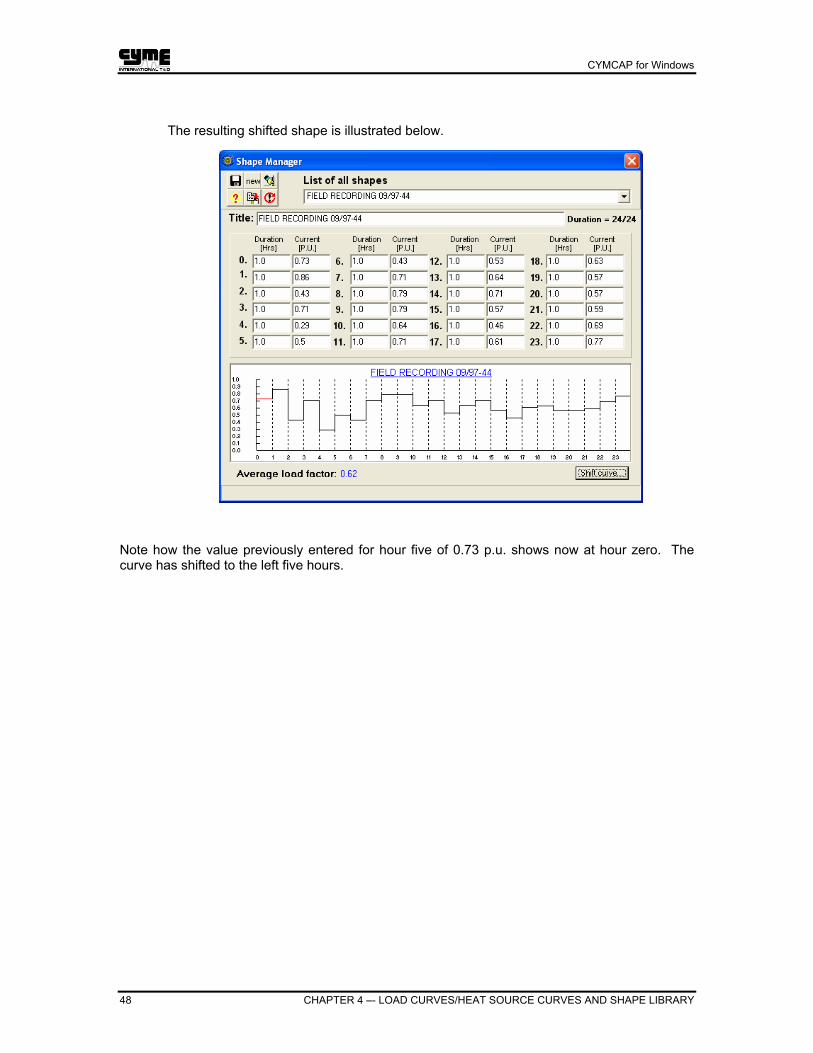
CYMCAP for Windows


The resulting shifted shape is illustrated below.

Note how the value previously entered for hour five of 0.73 p.u. shows now at hour zero. The curve has shifted to the left five hours.

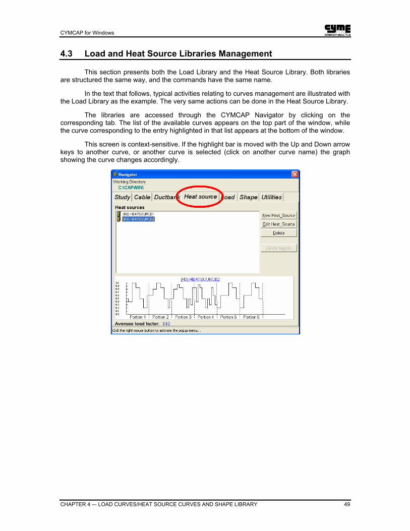
CYMCAP for Windows


4.3 Load and Heat Source Libraries Management

This section presents both the Load Library and the Heat Source Library. Both libraries are structured the same way, and the commands have the same name.

In the text that follows, typical activities relating to curves management are illustrated with the Load Library as the example. The very same actions can be done in the Heat Source Library.

The libraries are accessed through the CYMCAP Navigator by clicking on the corresponding tab. The list of the available curves appears on the top part of the window, while the curve corresponding to the entry highlighted in that list appears at the bottom of the window.

This screen is context-sensitive. If the highlight bar is moved with the Up and Down arrow keys to another curve, or another curve is selected (click on another curve name) the graph showing the curve changes accordingly.

CYMCAP for Windows


4.3.1 Expanding and collapsing the curves

To the left of every curve name a bitmap showing a closed drawer is displayed.

Double click on the curve name and the bitmap changes (the drawer opens)

while at the same time the sequence of shapes composing the Load Curve is displayed.

This action is called “expanding the curve”, and permits immediate identification of the shapes used by the current curve. The reverse action is called “collapsing the curve”. The numbers in parentheses shown to the right of every shape are the scaling factors applied to the shape within this particular curve.

After expanding the curve, if any shape is selected (click on the shape with the mouse, the shape title is highlighted and the appropriate section of the curve identified in the context-sensitive screen. You will also notice that the command buttons at the right of the window will now show “Shape” instead of “Load” or “Heat Source”.

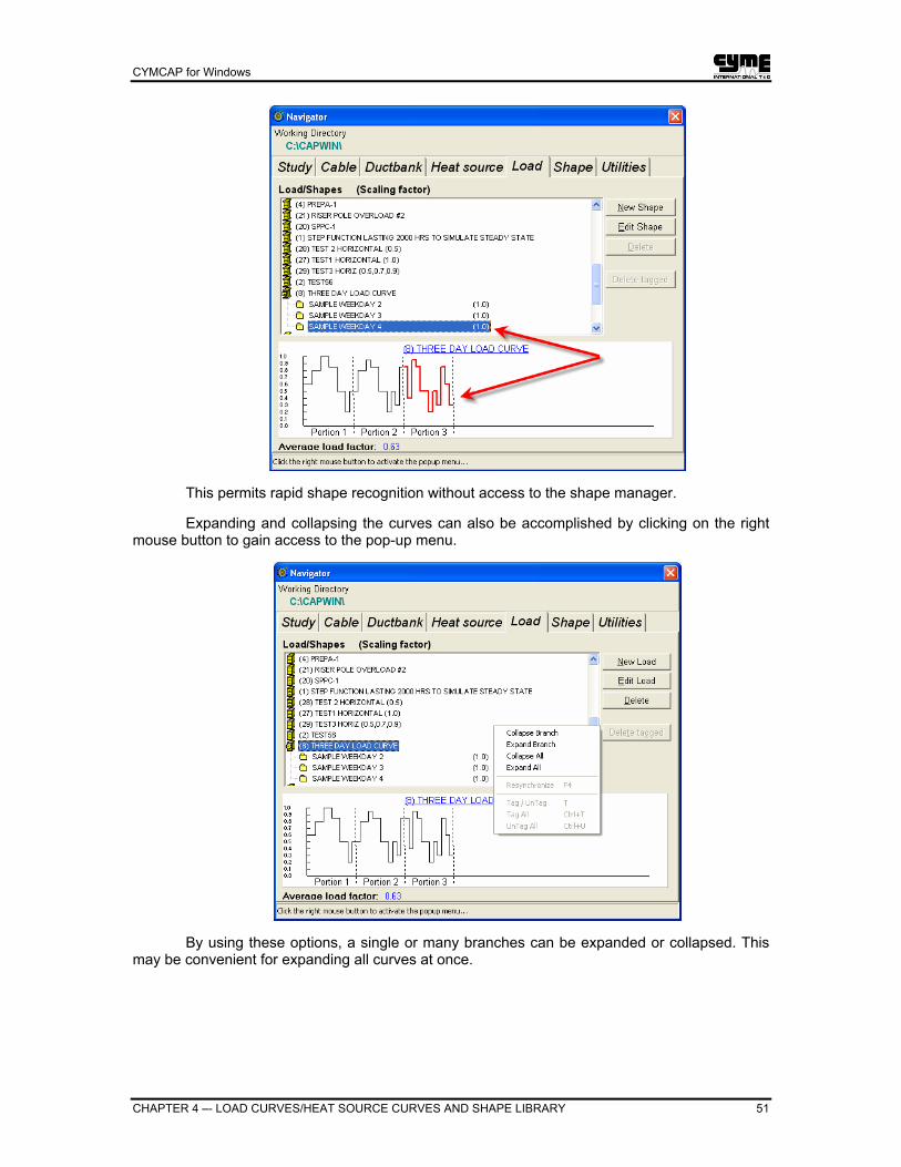
CYMCAP for Windows


This permits rapid shape recognition without access to the shape manager.

Expanding and collapsing the curves can also be accomplished by clicking on the right mouse button to gain access to the pop-up menu.

By using these options, a single or many branches can be expanded or collapsed. This may be convenient for expanding all curves at once.

CYMCAP for Windows


4.3.2 Curves libraries command buttons

To EDIT a curve, position the highlight bar on the curve to be edited and click on the Edit button to the right. You cannot edit a curve by double-clicking on it since this action is reserved for expanding/collapsing the curve. You can also display the curve to edit by clicking on the hyperlink appearing at the top of the graphical display of the curve.

To CREATE a new curve, position the highlight bar on any curve and click on the New button to the right. If you want to use any given curve as a template for the new one, position the highlight bar on the one to be used as a template.

To RENAME a load curve you must Edit it first.

To DELETE a curve, position the highlight bar on the curve to be deleted and click on the Delete button to the right. If that curve is used for any transient simulation a warning will follow.

4.3.3 Create a Load Curve using existing shapes – An illustrative example

Assume a new Load curve is to be created. This curve will portray a weekly variation. The curve therefore shall be composed of 7 portions. Each portion can have a different shape. The same shape can be used for different portions with identical or different scaling factors. For the example in question it is assumed that the shapes to be used have already been created.

Activate the CYMCAP Navigator and access the Load Library. Position the highlight bar on any Load curve and click on the New Load button.

CYMCAP for Windows


To the prompt asking if the current load curve is to be used as the template we respond No, which displays the Load Manager workbench with no shapes selected. When Yes is selected, the workbench is displayed populated with the data pertaining to the curve being used as the template.

First, the title of the curve is entered: A WEEKLY CURVE. Then, we start constructing the Load curves from the available shapes in the Shape library. The Load Manager workbench shows the list of shapes in the left part of the window, with the Shape(s) for current load field, empty. Select any shape in the Shape Library list by highlighting it. By clicking to the arrow pointing to the right , the highlighted shape is imported to the list of shapes composing the Load curve being constructed. The shape selected is now shown as the first portion of the Load curve being drawn.

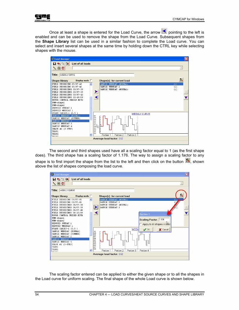
CYMCAP for Windows


Once at least a shape is entered for the Load Curve, the arrow pointing to the left is enabled and can be used to remove the shape from the Load Curve. Subsequent shapes from the Shape Library list can be used in a similar fashion to complete the Load curve. You can select and insert several shapes at the same time by holding down the CTRL key while selecting shapes with the mouse.

The second and third shapes used have all a scaling factor equal to 1 (as the first shape does). The third shape has a scaling factor of 1.176. The way to assign a scaling factor to any shape is to first import the shape from the list to the left and then click on the button , shown above the list of shapes composing the load curve.

The scaling factor entered can be applied to either the given shape or to all the shapes in the Load curve for uniform scaling. The final shape of the whole Load curve is shown below.

CYMCAP for Windows


The new Load curve can be saved and remain in the library for future utilization. The Load Manager workbench features several command buttons that summarize the various functions of the workbench.

More specifically:

Save the Load Curve with the modifications.

Import the Load Curve Data from a file (.DAT).

Delete the Load Curve.

Put a Load Curve in the windows clipboard.

Create a new shape.

Edit the highlighted shape.

These two commands give direct access to the Shape Manager workbench (see section 4.2 Shape Library management from the Load Manager workbench.

Revert to the original entries defining the Load Curve, once a modification was effected.

Shapes can be created while building the Load Curve

It is not necessary to have all the shapes available in the Shape Library in order to build the Load Curve. The Load Manager workbench does not only give access to the Shape Library but also to the basic functions of the Shape Manager via the Edit Shape and the Create New Shape buttons. Thus shapes can be created and modified while constructing the Load curve.

CYMCAP for Windows


Shapes can be assigned different scaling factors within a Load Curve

When a shape is used within a Load curve, a scaling factor can be applied to it. This scaling factor is applicable only for the given Load curve. The shape data within the shape library are left intact. If the same shape is used twice in a given Load curve with different scaling factors, the second scaling factor is applied to the original shape and not to the one entered previously in the load. Every time a shape is imported to a Load Curve the scaling factor is assumed to be 1.0 even if that shape has already been used with a different scaling factor.

Change the order of the shapes in the Load curve

Once a Load curve is constructed, the order of its shapes can be altered. The arrow

keys pointing Up and Down , situated to the right of the list of the shapes composing the Load Curve, are reserved for that purpose. Their function is essentially the same as the one reserved for the arrows and Keys used to build the Load Curve.

Select any shape within the Load curve with the mouse and by clicking on the arrow

, the shape will be displaced one position up in the list. The graph showing the Load Curve will also be refreshed accordingly. The inverse is accomplished by using the arrow key

pointing downwards. This way, any shape can assume any position within the Load curve and portions can be interchanged rapidly, to create new Load curves.

Shapes can be visualized while building the Load Curve

When building a Load curve, the list of shapes available in the shape Library are listed so that a selection can be made. The exact graph of the shape is not, however, available until a selection is made and the shape already imported. CYMCAP gives the user the possibility to take a look at any shape before actually importing the shape to the load curve. To do so, enable the Display mode check box, and select any shape of interest in the Shape library.

CYMCAP for Windows


4.3.4 Load Curve from field-recorded data

It is common that measurements over a period of time are taken to determine the actual loading pattern of a cable. These measurements are often carried out at a given rate, yielding measurements at regular time intervals. This can continue for several hours, or even days, until a quite detailed set of measurements reflecting the load variation is obtained.

CYMCAP is capable of interpreting these measurements so that a load curve can be constructed and used for transient ampacity studies. The following sections explain how the program accomplishes that function.

Field-Recordings and Data Acquisition

It is assumed that the recorded measurements are logged to an ASCII file. It is this file that the program uses as its input to construct the load curve. The format of this ASCII file is a free format, i.e. no specific record positions are required for the data. It is imperative however, that (a) no field is missing (b) fields are interpreted in the proper sequence and (c) fields are separated by at least one blank character (space). Tab separations are not valid.

Each record of this ASCII file is composed of 3 fields: the time field, the date field and the current intensity field. The program will assume this field sequence for any ASCII file provided as input data.

Time field The Time field indicates the exact time the measurement took place and is composed of 2 digits denoting the hour indicator followed by 2 digits denoting the minutes indicator, separated by a dot. No other format will be accepted. For example, 01.10 denotes a measurement which took place at 1:10 a.m., while 13.10 denotes a measurement that took place at 1:10 p.m. The valid range for the hour indicator is from 00 to 23 and for the minute indicator from 00 to 59.

Date field The Date field indicates the exact day and month the measurement took place and is composed of 2 digits denoting the month indicator followed by 2 digits denoting the day indicator, separated by a slash (/). For example, 08/09 denotes a measurement that took place on the ninth day of the eighth month. No other format will be accepted. No year indicator is supported. It is recommended, if the year is important, to include it in the Load curve title.

Current Intensity field

The Current Intensity field indicates the current that was measured on the date designated by the date field at the time designated by the time field. It is expressed in Amperes.

CYMCAP for Windows


Format Example: 00.00 08/08 55.00 01.10 08/08 60.00 13.25 08/08 50.00 13.45 08/08 60.00 14.02 08/08 50.00 14.22 08/08 60.00 15.01 08/08 40.00 15.32 08/09 60.00 15.57 08/09 34.00 16.32 08/09 40.00 16.43 08/09 60.00 22.22 08/09 33.00 23.59 08/09 14.00

Remarks on Constructing a Load curve from a Data file

• When constructing a Load Curve from a data file, each day is assumed to be a different portion having its own shape. There will therefore be as many different portions as the number of the defined days.

• If more than one measurement is obtained during one hour, the average of the recordings is taken as being the representative loading of the cable for that hour. If no measurement is recorded for the hour, a zero value of current will be assumed.

• If the load curve is supposed to span several days, no date is permitted to be missing from the starting date until the specified number of days is exhausted. The maximum number of days permitted in a Load curve is 7.

• When the Load curve is constructed and all the days with their 24-hour intervals defined, the interval with the maximum value of current is used to normalize the load curve. Thus, the interval with the highest recorded current value will appear as carrying a 1.00 p.u. current, while the rest of the intervals will feature a p.u. value which is found by dividing the actual current value for the interval by this maximum current value. The normalizing current is also indicated, once the calculations are completed. This piece of data can be useful when defining scale factors for the various cables in order to specify desired ampacity levels.

• The user can always edit the load curves produced from a recorded data file. It must be mentioned, however, that once this is done the modified load curve will not reflect the data contained in the data file which is associated with that load curve.

CYMCAP for Windows


Entering A Load Curve from an ASCII Data file

Activate CYMCAP, enter the navigator and access the Load Manager. Do not use the existing curve as a template and enter a title for the new curve as shown.

Then click on the Import from file button to activate the function to enter a Load curve from data recorded to an ASCII file. Select the directory in which the file with the recordings are located and select the file.

Then click on Open and the new Load curve will be constructed. The Load curve shown below is composed of three portions representing three days.

CYMCAP for Windows


When a Load curve is created from recorded data, new shapes are automatically created for each day in the file. These shapes are given default names and are automatically put in the Shape Library.

Note the above-described functionality is currently supported only for Load Curves. Heat source Load curves need to be entered using the Graphical User Interface. However, one can import the data of a Heat Source in an auxiliary Load to get the Shapes imported to the Shape Library. Then the user can use those imported shapes to build the Heat Source in the same way as a Load is built.

CYMCAP for Windows

CHAPTER 5 –- STEADY STATE THERMAL ANALYSIS 61

Chapter 5 Steady State Thermal Analysis

5.1 General

This chapter describes the necessary steps to perform steady state ampacity and/or temperature rise analysis. The available generic analysis options are outlined as well as the supported cable installations.

The term steady state means a continuous current for the cables just sufficient to produce asymptotically the maximum conductor temperature with the surrounding ambient conditions assumed constant.

5.2 Methodology and computational standards

CYMCAP deals with cables at all alternating voltages and direct voltages (up to 5kV). Cables can be directly buried, in ducts, in back fills, in through or steel pipes, as well as in air. The techniques and formulas outlined in the International standard IEC 60287, IEC 60853, IEC 60949 and IEC 1042 issued by the International Electrotechnical Commission are used throughout the calculations. The method of Neher and McGrath is used for non-unity load factors.

There are differences between CYMCAP and the IEC standards. Differences occur when we know of better (more accurate, more reliable, more detailed, etc.) computations. We should also point out that CYMCAP is frequently ahead of the IEC Standards and the improvements we implement eventually become part of the IEC standards. CYMCAP includes the following analysis options not directly addressed in the IEC standards:

a. Cables without metallic sheath, but with copper concentric wires bonded and grounded at one or both ends.

b. Submarine cables with touching steel armour wires with or without copper concentric neutral wires and without metallic sheath.

c. Cables on riser poles in a protective guard or duct.

d. Single-phase circuits consisting of one single core cable with concentric neutral wires or sheath serving as the return conductor.

e. Modeling of rectangular duct banks and backfills of any size by the extended geometric factor.

f. Modeling of soil drying out in the vicinity of the cable surface (moisture migration).

g. Modeling of non-isothermal earth surface conditions.

h. Paper-polypropylene-paper laminated cables.

i. Thermal analysis of grouped cables in the presence of solar radiation.

j. Multiple cables per phase.

k. Cables in magnetic ducts/risers

l. Cables on riser poles with different venting conditions.

m. Multiple duct banks, multiple backfills and multiple soil layers thought the MDB add-on module described in Chapter 11.

CYMCAP for Windows

62 CHAPTER 5 –- STEADY STATE THERMAL ANALYSIS

The permissible current rating of an AC cable is derived from the expression for the temperature rise above ambient temperature:

∆θ λ λ λ= + + + + + + + + +( . ) ( ( ) ) ( ( ) ) ( )I R W T I R W nT I R W n T Td d d2

12

1 22

1 2 3 405 1 1

Where:

I = Current flowing in one conductor (A)

∆θ ϑ ϑ= −c amb = Conductor temperature rise above ambient (°C)

R = ac resistance per unit length of the conductor at maximum operating temperature (Ω/m)

Wd = Dielectric loss per unit length for the insulation surrounding the conductor (W/m)

T1 = Thermal resistance per unit length between conductor and sheath (°C-m/W)

T2 = Thermal resistance per unit length of the bedding between sheath and armour (°C-m/W)

T3 = Thermal resistance per unit length of the external serving of the cable (°C-m/W)

T4 = Thermal resistance per unit length between the cable surface and the surrounding medium (°C-m/W)

n = Number of load-carrying conductors in the cable (equal size conductors carrying the same load)

λ1 = Ratio of losses in the metal sheath to total losses in all conductors in that cable

λ2 = Ratio of losses in the armor to total losses in all conductors in that cable

The permissible current rating is obtained from the above formula as follows:

I W T n T T TRT nR T nR T T

d=− + + +

+ + + + + +∆θ

λ λ λ( . ( ))

( ) ( )( )05

1 11 2 3 4

1 1 2 1 2 3 4

CYMCAP for Windows


The drying out of the soil is represented by computing the ampacity from the formula:

I W T n(T T TRT nR T nR T T

d x=− + + + −

+ + + + + +∆ ∆θ ν θ

λ λ λ ν( . ))( )

( ) ( )( )05 1

1 11 2 3 4

1 1 2 1 2 3 4

where:

∆θ θ ϑx x amb= − = temperature difference between critical isotherm (50°C) and the ambient (critical isotherm is one at which drying out occurs)

ν = ratio of thermal resistivities of dry and moist soil

The non-isothermal surface is modeled by an imaginary layer of soil d meters thick at the earth surface, where

d ar= 100

.

where:

a = convection coefficient

r0 = thermal resistivity of the moist soil

The convection coefficient is computed by the program.

CYMCAP for Windows


5.3 Accuracy of CYMCAP and References

The following figure shows the results of experiments made to validate the equations in CYMCAP for underground cables. It can be seen that the simulated and measured results match with reasonable accuracy.

Comparison of test measurements and CYMCAP

The numerical results of CYMCAP have been validated in the following ways: (1) The IEC standards are based for steady state computation on the Neher/McGrath

paper [1] and for transient computation on the Neher paper [2]. They performed experimental verification of their equations.

(2) The Canadian Electricity Association (CAE) performed substantial field verifications

in the 1980’s for the early CAP versions. These verifications were made mainly for underground cables [3]. The figure above corresponds to one of the tests.

(3) Phillips Cables (today, Northern Cables) compared the numerical results of the

earlier versions of CYMCAP with experimental tests for cables in air [4]. The simulations very closely matched the measured values; see the table below.

Shield Temperature [°C] Ampacity [A] Conductor

Temperature [°C] Actual CYMCAP Actual CYMCAP 90 76.0 73.6 810 817

130 102.0 102.6 1005 1004

Comparison of numerical and experimental results for cables in air

(4) Verifications with a finite elements program were carried out in [3], the figure and table below show a duct bank installation and the comparisons made with Massif, the finite elements program developed by IREQ the research institute of Hydro Quebec.

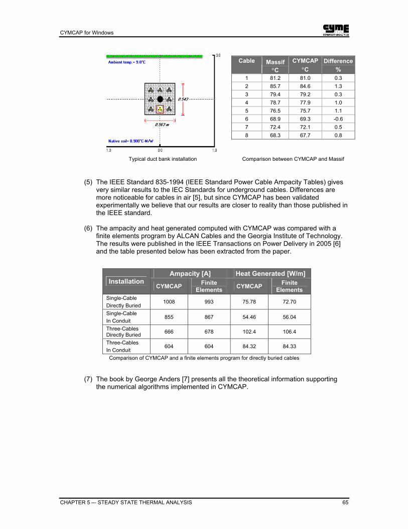
CYMCAP for Windows


Cable Massif

°C CYMCAP

°C Difference

% 1 81.2 81.0 0.3 2 85.7 84.6 1.3 3 79.4 79.2 0.3 4 78.7 77.9 1.0 5 76.5 75.7 1.1 6 68.9 69.3 -0.6 7 72.4 72.1 0.5 8 68.3 67.7 0.8

Typical duct bank installation Comparison between CYMCAP and Massif

(5) The IEEE Standard 835-1994 (IEEE Standard Power Cable Ampacity Tables) gives very similar results to the IEC Standards for underground cables. Differences are more noticeable for cables in air [5], but since CYMCAP has been validated experimentally we believe that our results are closer to reality than those published in the IEEE standard.

(6) The ampacity and heat generated computed with CYMCAP was compared with a

finite elements program by ALCAN Cables and the Georgia Institute of Technology. The results were published in the IEEE Transactions on Power Delivery in 2005 [6] and the table presented below has been extracted from the paper.

Ampacity [A] Heat Generated [W/m]

Installation CYMCAP Finite

Elements CYMCAP Finite Elements

Single-Cable Directly Buried

1008 993 75.78 72.70

Single-Cable In Conduit

855 867 54.46 56.04

Three-Cables Directly Buried 666 678 102.4 106.4

Three-Cables In Conduit

604 604 84.32 84.33

Comparison of CYMCAP and a finite elements program for directly buried cables

(7) The book by George Anders [7] presents all the theoretical information supporting

the numerical algorithms implemented in CYMCAP.

CYMCAP for Windows


5.3.1 References

[1] J.H. Neher and M.H. McGrath, “The Calculation of the Temperature Rise and Load Capability of Cable Systems”, AIEE Transactions Part III - Power Apparatus and Systems, Vol. 76, October 1957, pp. 752-772.

[2] J.H. Neher, “The Transient Temperature Rise of Buried Cable Systems”, IEEE Transactions on Power Apparatus and Systems, Vol. PAS-83, February 1964, pp. 102-114.

[3] Canadian Electrical Association, "Ampacity Calculation on Power Cables & Cyclic Loading for Distribution Cables in Duck Bank – Volume I: Overview of the Technical and Experimental Developments", Contract No. 138-D-375 and No. 137-D-374, October 1986

[4] Phillips Cables, "FIECAG Ampacity Program – Evaluation Phase I, Engineering Report No. 87-30, December 1987.

[5] IEEE Standard Power Cable Ampacity Tables, IEEE Std 835-1994. [6] P. Vaucheret, R.A. Hartlein, and W.Z. Black, "Ampacity Derating Factors for Cables Buried in

Short Segments of Conduit", IEEE Transactions on Power Delivery, Vol. 20, No. 2, April 2005, pp. 560-565.

[7] George Anders, “Rating of Electric Power Cables: Ampacity Computations for Transmission, Distribution, and Industrial Applications”, IEEE Press, 1997, ISBN 0-7803-1177-9. It is now available through McGraw-Hill only.

5.4 Studies and executions

A typical example of this categorization scheme is the case of analyzing the effect of bonding and/or transposition for the sheaths of single core cables in a three-phase circuit. Although the basic installation remains unaltered, one may define several executions each with different bonding arrangement to best investigate the effects of bonding. When a study is created for the first time, an execution is also automatically created.

STUDIES

Study no. 1, Study no. 2, ..............................Study no. xx, ....

Execution no. 1, ..n ........ Execution no. 1, ..n

A study may contain as many executions as needed.

CYMCAP for Windows


5.5 Library of studies and executions

Much like the various types of cables, the studies are kept in a separate library. This section describes how to enter a new study in the library and how to manage an existing library of studies. Access to the library of studies allows the user not only to add a new study but also to modify and even delete previously entered ones.

The library of studies is accessed through the CYMCAP Navigator clicking on the Study tab. The top part of the window displays the list of studies that can be expanded afterwards to show the executions that are part of that study. To expand the list, double-click on the name of the study, or right-click to display the context-sensitive menu and select Expand.

Studies are represented by a filing cabinet icon (closed when the branch is collapsed

and open when the branch is expanded). When the list is expanded, each execution is

represented by a folder icon .

The bottom part of the window is a viewer used to display the executions. If you wish, you may hide this part by checking the View installation checkbox; the list of studies will then occupy the complete space.

When an execution from the list is selected (or a study with only one execution) the installation will be displayed in that window. This serves to avoid opening an execution to graphically see the installation.

CYMCAP for Windows


Four check boxes appear on the main window:

View execution number

This will show the execution number of the open execution screen (after clicking on Edit).

View cable(s) installed for each execution

With this check box enabled, the list of cables part of the executions will be displayed when the command Expand branch or Expand all will be selected from the Study pop-up menu. (see below).

View installation To display or hide the graphical viewer pane at the bottom of the window.

Hide on edit Un-checking this box does not close the Navigator when an execution is being edited.

To EDIT a study, position the highlight bar on the study of interest and click on the Edit button to the right. Double clicking on the study will not resort to editing since this function is reserved for expanding/collapsing the study. When a study is edited all executions within the study are brought up for editing. Data pertaining to any execution can then be modified accordingly.

To DELETE a study you position the highlight bar on it and click on the Delete button to the right. When a study is deleted ALL the executions belonging to this study will be deleted.

To CREATE a new study, position the highlight bar on any study and press the New Study button to the right. When a new study is created, you have the choice to use that study as a template or create from scratch a completely new one. See 5.6 Creating a study for details.

To CREATE a new execution within the study, select any existing execution as a template to create the new execution. The execution highlighted will always be used as template. The only way to create a completely new execution without using any templates is to create a new study.

5.5.1 Study library pop-up menu

CYMCAP for Windows


Search Utility Allows finding a specific study, execution, or cable using alphanumeric string to filter out the studies by name. The library of studies can be quite voluminous. Once, accessed it can be difficult to locate a particular study of interest. That is why CYMCAP features a search facility that is activated by mouse right-clicking.

Once you click on the Find button, the program will perform the search and tag all entries that comprise the string searched.

The studies do not need to be expanded for the search facility to be operated. The search facility can be case sensitive OR pertain to tagged library entries only. The search facility can be a forward/backward search OR a global search.

Note that performing a search will automatically enable the Tag mode. To disable it, uncheck the corresponding checkbox in the CYMCAP utilities.

View All Selecting this option will list all the studies in the Study Library list.

View Tagged Only This is used to view only the studies (and the eventually the executions) that are “Tagged”. The Tag mode needs to be enabled first; this is done though the CYMCAP Utilities, which are described in Chapter 9.

Sort by Study Id Sorts the displayed study entries on the list by Study ID. (The ID of a study is shown between brackets to the left of the study name).

CYMCAP for Windows


Sort by Study Title Sorts the displayed studies by study title.

Cut Removes studies/executions to be copied into other studies

Copy Copies studies/executions

Paste Adds cut or copied studies/executions into other studies

Collapse Branch To hide the list of executions part of the study, which name is highlighted.

Expand Branch To display the list of executions part of the study, which name is highlighted. When the View cable(s) installed for each execution checkbox is checked, the cables part of each execution displayed with this command will also be displayed.

Collapse All To hide all the lists of executions part of the studies listed.

Expand All To display the list of executions part of all studies listed. When the View cable(s) installed for each execution checkbox is checked, the cables part of each execution displayed with this command will also be displayed.

Print Selected Branch…

To print the list of executions of the study for which the name is highlighted in the list.

Print only Expanded Branches…

To print the list of only the studies which are expanded to show their executions.

Print All Branches…

To print the complete list of studies, each with their list of executions.

Resynchronize This function operates only in multi-user network licenses. It serves to refresh the list of cables.

Tag/UnTag To select (tag) or unselect (remove tag) a cable. Active when the Tag mode has been enabled (in the Utilities window).

Tag All To selects all cables in the view. Active when the Tag mode has been enabled.

Untag All To unselects all cables. Active when the Tag mode has been enabled.

Expanding a study is a convenient way to view the executions available for a particular study. Another important piece of information is the type of cable(s) used within a given execution. CYMCAP offers the possibility to access the cable types without resorting to detailed execution editing, thus circumventing the necessity to memorize execution titles. Click on the button “View cable(s) installed for each execution”, and the type of cables associated with the execution is shown.

CYMCAP for Windows


Bitmaps are used to portray the various types of cables, as follows:

Single Core self-contained cables.

Pipe type cables cradled configuration within the pipe.

Pipe type cables triangular (trefoil) configuration within the pipe.

Three core self-contained cable.

Three core self-contained with sector-shaped conductors.

CYMCAP for Windows


5.6 Creating a study

Whenever you create a new study, your will have the choice of using the study highlighted in the list as a template or to create a brand new one.

If you use the study highlighted as your template, you will be prompted to label that new study with a unique study ID and Title only.

If you create a brand new study, you will be prompted to enter a short description of your execution no. 1 as well.

In order to label a study and/or execution, you need to supply:

ID This is the unique Study ID. It consists in an alphanumeric string, 10 characters long. Use different ID's for different studies for better study identification. CYMCAP uses the STUDY ID for Data Base management purposes only.

Title This is the study title. It is an alphanumeric string 60 characters long to be used as the study title. Use different titles for different studies, for better study identification. Used by CYMCAP to list the various studies.

Execution Title

This alphanumeric string of 60 characters long is used as the execution title. Different executions should have different titles for better execution identification.

Comments This field is used to enter any additional important information that needs to be remembered about a particular execution.

CYMCAP for Windows


Date When an execution is created, the date for the execution remains blank by default. The user can indicate a specific date for an given execution using this command.

CYMCAP provides a calendar synchronized with the computer clock. Access it and any desired date can be entered.

Executions within a study are internally numbered consecutively. To view the execution numbers when editing one or more, you need to enable the appropriate option in the navigator screen; otherwise the execution number is not displayed on the editing screen, but only the title is displayed.

CYMCAP for Windows


5.7 Analysis options

CYMCAP offers the following two analysis options:

1. STEADY STATE THERMAL ANALYSIS, for calculations of ampacities and/or temperature rises when the cable currents are not functions of time. For temperature rise calculations, the currents in the cables are specified and temperatures are sought. For Ampacity calculations, the maximum permitted conductor temperatures are entered and the cable currents are sought. Hybrid calculations are also supported. That means that ampacities can be computed for several circuits while assuming fixed current values for the remaining.

2. Cyclic Loading in CYMCAP can be performed as part of a steady state analysis. CYMCAP allows the use of load factors. The load factor is used as per the two common cyclic loading approaches:

a. Neher-McGrath

b. IEC 60853

For many years only the Neher-McGrath approach was supported in CYMCAP and therefore it is the default selection. In 2006 (for version 4.3) Cyclic Loading as per IEC 60853 was introduced. If a user would like to run cyclic loading with this option, he/she needs to change it manually as illustrated next.

There are important differences between the two approaches and the user should be aware that different results are expected. The Neher-McGrath approach considers cyclic loading by adjusting T4 (the external to the cable thermal resistance), while the IEC 60853 uses a cyclic factor M. In the former moisture migration cannot be included in a simulation, while in the latter it can.

3. TRANSIENT ANALYSIS, for calculations where the cable loading is a function of time, and/or transient conditions are sought. Transient calculations must be preceded by Steady State analysis. No transient analysis is supported for installations of cables in air and in the presence of moisture migration.

The remaining sections in this Chapter covers at length the Steady State Thermal Analysis options, while Chapter 6 covers the complete subject of Transient Analysis.

CYMCAP for Windows


5.8 Steady state analysis

In the first stage of a steady state analysis, the user is prompted for the specific analysis option that is to be exercised. The choice of this option determines the data to be asked for the cable installation.

The Steady state analysis options available in CYMCAP are:

1 EQUALLY LOADED

If the installation comprises only IDENTICAL cables which are equally loaded.

This is the default option.

2 UNEQUALLY LOADED

If the installation comprises unequally loaded and/or dissimilar cables.

FOR OPTIONS 1 AND 2 THE MAXIMUM CONDUCTOR TEMPERATURES ARE SPECIFIED AND THE PROGRAM CALCULATES CABLE AMPACITIES.

3 TEMPERATURE If the conductor currents are known and the temperatures are sought.

FOR THIS OPTION THE CABLE CURRENTS ARE SPECIFIED AND THE PROGRAM CALCULATES THE CABLE TEMPERATURES.

If in the study some cable currents are to be kept constant, while calculating maximum temperatures, choose option 2.

The following subsections explain in detail the data to be considered when preparing a steady-state analysis:

• General data for the installation (section 5.8.1)

• Cable Installation data (section 5.8.2)

• Specific cable installation data (section 5.8.3)

The functionality offered by CYMCAP for steady state analyses is described with study cases. These outline several major analysis options of the program. The basic interface aspects of CYMCAP associated with this analysis option are presented there.

• Steady state thermal analysis, Example 1: Cables in a duct bank (section 5.10)

• A study case for dissimilar directly buried cables (section 5.11)

• Specific installation data (section 5.12)

CYMCAP for Windows


5.8.1 General data for the installation

5.8.1.1 Ambient temperature and soil resistivity

AMBIENT TEMPERATURE and SOIL RESISTIVITY values should correspond to the installation situation and not necessarily to the test condition of the manufacturer. Ambient temperature for buried cables is the soil ambient temperature at the cable burial depth, and the air ambient temperature if the cables are installed in air, or non-isothermal earth modeling is desired.

Soil thermal resistivities range, typically, from 0.8 to 1.3 °C-m/W. Values as low as 0.4 and as high as 4 C-W/m can also be encountered. The thermal resistivity of the soil is a very important factor affecting cable ampacity, particularly for directly buried cables. The higher the soil thermal resistivity, the lower is the ampacity, for a given maximum permitted conductor temperature. Thermal resistivity increases with decreasing moisture in the soil. The thermal resistivity of dry sand can be as high as 5 C-m/W, while, thermal resistivity of dry crushed limestone, usually, cannot be higher than 1.5 C-m/W. Soil thermal resistivity is also inversely proportional to the degree of the soil compacting.

If the soil thermal resistivity is unknown, the value of 1.3 can be used as an average conservative estimate. The IEEE Standard 442-1981, “IEEE Guide for Soil Thermal Resistivity Measurements” provides a procedure to measure the thermal resistivity of the soil. Some of the materials listed in the standard are given in the table below.

Material Thermal

Resistivity [°C-m/W)

Quartz Grains 0.11 Granite Grains 0.26 Limestone Grains 0.45 Sandstone Grains 0.58 Mica Grains 1.70 Water 1.65 Organic Wet 4.00 Organic Dry 7.00 Air 40.00

5.8.1.2 Non isothermal earth surface modeling

NON ISOTHERMAL SURFACE MODELING may be necessary for the case where the cables are buried relatively close to the surface of the earth. The implication of this is that the earth surface can no longer accurately be considered as an isothermal.

For non-isothermal surface modeling, the program needs the air ambient temperature. THIS TEMPERATURE MUST BE GREATER THAN THE SOIL AMBIENT TEMPERATURE. Non-isothermal earth surface modeling is warranted only if d/L <0.4, (d is defined in section 5.2, Methodology and computational standards’ and L is the depth of burial of the cable closest to the earth surface) and the user wishes to do so. If all the cables in the installation are located at a depth greater than 1.5 m, non-isothermal modelling is considered unnecessary.

CYMCAP for Windows


5.8.1.3 Moisture migration modeling

MOISTURE MIGRATION, also referred to as "drying out of soil", in the vicinity of the cable surface is modeled, if the user wishes. In this case, the user will be asked to enter dry soil thermal resistivity.

The dry soil thermal resistivity value is larger than the ones usually assumed for moist conditions and can be as high as 4.0 degrees °C-m/W. The program assumes by default that the critical temperature at which moisture migration occurs is 50°C if the user does not specify this value. The IEEE standard 442 provides curves of soil thermal resistivity versus moisture content.

Notes:

• Moisture migration is not supported for cables in ducts, and for cables in backfill.

• No transient analysis can be carried out in the presence of moisture migration.

5.8.1.4 Surrounding medium of the installation

This is to specify whether the cables are directly buried, in backfill, ducts or in air. Depending on the particular installation, the following additional data may be necessary:

Backfill/Ductbank data Backfill data pertain to thermal backfills and duct banks. The basic version of the program cannot handle more than two different materials surrounding the cable. Through the MDB add-on module described in Chapter 11 the user can model up to 12 materials or regions with different thermal resistivities. Rectangular backfills/duct banks are the only types supported by the basic program. The MDB add-on module also allows the modeling of soil layers. Its dimensions and thermal resistivity characterize a backfill or a duct bank. The thermal resistivity of the backfill is usually lower than the native soil. The thermal resistivity of concrete is usually in the range of 0.5 to 0.8 °C-m/W. The coordinates for the Backfill/Duct bank center must be based on the same reference axes as the cable coordinates. It is emphasized, again that no moisture migration is supported when the cables are contained in a backfill or duct bank.

Caution Notes:

(1) The permitted duct bank width/height ratio in the Neher-McGrath method goes from 1/3 to 3. If the entered width and height values give a greater or smaller ratios CYMCAP uses published extensions obtained with finite elements.

Since there is a change of calculation method when exceeding the upper or lower limit, users performing parametric studies might find that the computed ampacity behaves strangely. The results obtained from the extension formula are considered to be more accurate.

(2) Please be aware that in both cases, the Neher-McGrath and the extensions, it is assumed that the duct bank or backfill surface is an isothermal. This assumption most probably is not true for very large or small ratios of width to height (larger than 5). Also the assumption might not be fulfilled when the duct back/backfill is close to the surface. Please use the results having the mentioned limitations in mind.

(3) To avoid the problems described in points (1) and (2) the calculations can be accurately performed with the Multiple Duct Bank (/MDB) add-on module.

CYMCAP for Windows


Cables in air When cables are installed in air, besides the data pertinent to solar radiation, the program needs to know if any special cable arrangement applies.

1. SOLAR RADIATION MODELING is supported only for the case the cables are installed in air and are "unshaded". The user needs to enter the following information:

a) Intensity of solar radiation in W/m2, or in W/ft2. The value depends on the latitude and altitude of the installation, the day of the year and the sky conditions. CYMCAP can compute the intensity of solar radiation when it is unknown (see below).

b) Absorption coefficient for the cable surface material. The following are typical values for various materials:

Compounded jute/fibrous materials ABSC = 0.8 Polycholoroprene ABSC = 0.8 Polyvinylchloride ABSC = 0.6 Polyethylene ABSC = 0.4 Lead or armour ABSC = 0.6 Steel ABSC = 0.55

c) For cables installed in air, the load factor has to be 1.0.

CYMCAP has a facility to compute the solar radiation intensity for a given location using the ASHRAE Clear Day Solar Flux Model published originally in the ASHRAE Handbook of Fundamentals. Several known improvements have been made for its inclusion in CYMCAP. When clicking on Compute solar radiation in the Cables in Air dialog box, a new dialog box will open to enter the geographical and date information in order to obtain the intensity of solar radiation for the specified location, day and sky conditions.

CYMCAP for Windows


2. SUPPORTED CONFIGURATIONS FOR CABLES INSTALLED IN AIR. The following table illustrates the cases that CYMCAP supports for cables near or clipped to walls. The necessary assumptions concerning clearances are also tabulated. These cases are directly taken from the IEC287 standard.

For configurations 1 to 10 outlined in the figure, the following applies:

• Cables are assumed in free air or non-continuous brackets, ladder supports or cleats.

• “De" is not greater than 0.15m.

• Values for 1 cable also apply to each cable of a group when spaced horizontally, with a clearance between cables of at least 0.75 times the overall cable diameter.

Groups of cables in air per IEC-1042

CYMCAP for Windows


The available choices for groups of cables in air are shown in the figure below. These configurations have been obtained from the IEC standard 1042 (1991). The calculating procedures contained in IEC-1042 have been modified to take into account solar radiation.

NOTE: All the cables must have the same Cable ID.

Cables on riser poles Cables on riser poles are installed in vertical arrangements with a guard to provide mechanical protection. These guards act as ducts for thermal analysis purposes. However, since the heat transfer mechanisms are different for those arrangements, as compared to horizontally placed ducts, in order to avoid overestimation of the ampacities for cables on risers, CYMCAP uses a dedicated methodology to treat cables on riser poles.

As the following table indicates, the program supports both-ends vented guards, partially vented (open at the top) and completely closed risers. The possibility of having 1 or 3 cables in the riser guard is also supported for all three cases.

When magnetic risers are considered, all 3 phases must be present. In other words, we can either have:

a) 3 single-core cables in trefoil within the same duct, b) a 3-core cable in a duct, or c) 3 single-core cables in 3 different ducts spaced apart.

For the former 2 cases, enter in Cable installation data the coordinates of the center of the duct, while for the third case all three cables must be explicitly entered, respecting their spacing. For 3 single-core cables in the same duct, select the appropriate icon (2, 4 or 6) and enter only one cable in the cable installation data. The program will assume that 3 cables in trefoil are considered. The bitmaps shown for cables on riser poles are generic. Thus,

CYMCAP for Windows


a 3-core cable can also be modeled in the guard by choosing options 1, 3 or 5, despite the fact that the icons portrays single-core cables.

Heat/Sink Source Modeling This option can be exercised to model a nearby heat source (or sink) that is suspected to be influencing the ampacity calculations. This can be used for nearby steam pipes, waterbeds etc. There are four possibilities:

a. Source inside backfill specified as constant temperature.

b. Source inside backfill specified as heat flux source.

c. Source not in backfill specified as constant temperature.

d. Source not in backfill specified as constant heat flux.

Heat flux is expressed in W/m2 and temperature in °C. Heat sources are modeled as circles with either constant temperature or constant heat flux boundaries. When therefore a source is specified, the source coordinates and the diameter are the data required. If the source is in backfill, make certain that the source circumference falls within the backfill. Similarly, if the source is specified outside the backfill make sure that the source circumference stays completely out of the backfill. No hybrid geometrical situations are recommended.

An insulation layer can be added to a heat source (sink) when the temperature is specified for steady state ampacity or temperature simulations. Heat sources are supported in transients, but with no insulating layer.

CYMCAP for Windows


5.8.1.5 Multiple cables per phase

Some installations feature more than one cable, in parallel, per phase. This is normally due to the fact that the load per phase may be too high to be carried by a single cable. We may therefore have 2, 3 or more cables per phase. When single core cables are connected in parallel, the load current may not share equally between them, due to the fact that the associated impedances are not only a function of the self but of the mutual inductance between cables and their sheath which is dependent on the geometrical arrangement. Similar considerations apply for the circulating currents in their sheaths for 2-point bonded systems. In calculating ampacities for cables in parallel, different sheath loss factors are involved. Their value depends not only on the cable location, but also on the phase labeling as well.

Modeling installations that involve several cables per phase by assuming every parallel path to be an independent circuit entails an error because this will disregard the mutual impedances between sheaths of the same circuit and could result in overestimating the cable ampacities.

Notes:

• All the cables for multiple cables per phase will have to be the same cable type when they belong to the same circuit. Different circuits can, however, have different cable types.

• Multiple cables per phase cannot be applied on 3-core cables.

• The notion of transposition, cross-bonding and minor section lengths as well as specifying section length for 2-point bonded systems are not applicable.

5.8.2 Cable Installation data

This part of data entry pertains to the geometrical coordinates of the cables used in the installation and comprises labeling and cable numbering conventions the application abides by. Depending on the analysis option selected for steady state analysis, conductor temperatures may need to be entered instead of conductor currents.

5.8.2.1 Geometrical configuration of the installation

The geometrical location of the cables, i.e. their coordinates is necessary.

The Y-coordinate value for the cables is always assumed to be positive and designates the depth of burial with respect to the earth surface which is assumed at Y=0.0. For cables installed in air, Y can be set to 0.

The X-coordinate values can be either positive or negative. The choice of the origin of the X-axis should be governed, whenever possible, by the ease of entering cable coordinates. It is common for installations to exhibit symmetry along a vertical axis. Choose this vertical axis to be the X-axis reference. This will at first greatly facilitate entering the coordinates (half the cables will be mirror images of the other half) and at second it will ease the convergence process.

Note that entering the X and Y coordinates for every cable is not always necessary since that in some cases only distances between the various cables is of importance. In other cases, the coordinates of only one cable are necessary, while the rest can be deduced from the cables spacing.

CYMCAP also allows the user to enter the coordinates for a cable in relative coordinates by designating any cable in the installation as the beacon cable.

CYMCAP for Windows


5.8.2.2 Additional cable installation salient aspects

The circuit number identifies the 3 phases of the circuit. If more than one cable share the same circuit number, the program will check if there are 3 cables and if all are of the same type. If not, the user will be requested to correct the data.

The cable design ID is the IDENTIFICATION string given to cable in the cable library. The cable ID is used in the installation data because it is shorter than the cable title. The cable library is accessible when entering the cable installation data as the examples that follow clearly show. You cannot select for the installation a cable that is not in the library. Make certain that cables with the same circuit number have the same cable ID.

A maximum of 45 cables can be entered per installation. If cables are in a duct bank, with three cables per duct, only one cable is sufficient to represent the trefoil formation. CYMCAP will automatically designate that CABLES ARE TOUCHING in the specific installation data (see below). The implicit assumption of this modeling is that all three phases are in the same duct. Similarly, for the case of 3 cables which are directly buried or in backfill and they are touching (i.e. the cables are in a triangular formation directly in contact) CYMCAP facilitates data entry by entering the coordinates of the center of the trefoil formation. In the Specific cable installation data CYMCAP shall designate the cables as “touching".

5.8.2.3 Cable Installation types

CYMCAP supports the following generic types of cable installations:

• Cables in air

• Cables in duct/duct is in air.

• Cables directly buried.

• Cables in thermal backfill.

• Cables in ducts or in an underground duct bank.

• Cables in pipe and the pipe directly buried.

• Cables in pipe and the pipe in thermal backfill.

• Cables installed in multiple duct banks, multiple backfills and/or multiple soil layers with different thermal resistivities*.

This information is used to direct the program for any additional data required. Pipe-type cables are always assumed to be three-conductor cables.

* The ampacity for cables in multiple duct banks, multiple backfills and multiple soil layers with different thermal resistivities is computed using an add-on module (see all the details in Chapter 11).

5.8.3 Specific cable installation data

This data is used to provide further details about the installation pertaining to specific cable types used in the installation.

An installation may have many cables, but only a few types of cables. Specific installation data have to be entered for every cable type. Once specific installation data is specified for one cable type, the information remains for all cables of this type in the installation.

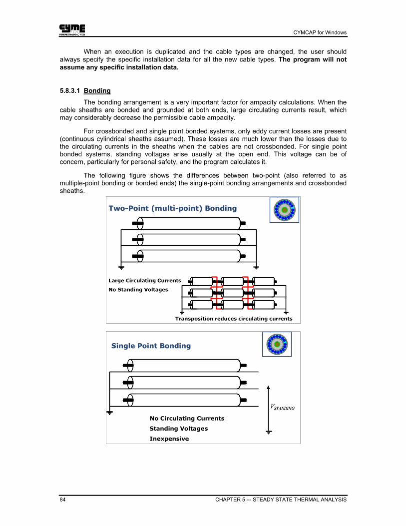
CYMCAP for Windows


When an execution is duplicated and the cable types are changed, the user should always specify the specific installation data for all the new cable types. The program will not assume any specific installation data.

5.8.3.1 Bonding

The bonding arrangement is a very important factor for ampacity calculations. When the cable sheaths are bonded and grounded at both ends, large circulating currents result, which may considerably decrease the permissible cable ampacity.

For crossbonded and single point bonded systems, only eddy current losses are present (continuous cylindrical sheaths assumed). These losses are much lower than the losses due to the circulating currents in the sheaths when the cables are not crossbonded. For single point bonded systems, standing voltages arise usually at the open end. This voltage can be of concern, particularly for personal safety, and the program calculates it.

The following figure shows the differences between two-point (also referred to as multiple-point bonding or bonded ends) the single-point bonding arrangements and crossbonded sheaths.

TwoTwo--Point (multiPoint (multi--point) Bondingpoint) Bonding

Large Circulating Currents

No Standing Voltages

Transposition reduces circulating currents

Single Point BondingSingle Point Bonding

VSTANDINGVSTANDING

No Circulating Currents

Standing Voltages

Inexpensive

CYMCAP for Windows


Cross BondingCross Bonding

No Circulating Currents

No Standing Voltages

Installation Expensive – Reduced Losses Crossbonding can be applied with equal or unequal section lengths. In the former case,

circulating currents are the minimum while in the latter some circulating currents may exist. In the case of unequal section lengths, the program requests the user to use the length of the shortest section as reference and define the remaining two sections (longer and longest) by using the length ratios longer/shortest (AN) and longest/shortest (AM) to quantify the degree of asymmetry and thus calculate the circulating currents in the sheaths accordingly.

Concentric wires shields and sheath reinforcement assemblies follow the bonding option selected for the sheaths. For single-point bonded and cross-bonded systems only sheath and sheath reinforcement eddy currents are considered as losses. Armour wires are always assumed to be bonded and grounded at both ends. Non-magnetic armour is combined with the sheath for circulating current loss computations. Non-magnetic armour wires, in the absence of a sheath should always be modeled as concentric neutral wires.

Since it is not always possible to install cables with one value of spacing along a given route, the program supports unequal spacing of cables. The following relate to the calculation of sheath circulating current losses for 2-point bonded systems when a situation like this occurs. A section is defined as the length along two points of the cable route where shields are solidly bonded. Loss factors have to be calculated based on conductor and external thermal resistance of the closest cable spacing along the section.

a) When spacing along a section is not constant but the various lengths are known, the value for X are derived as per IEC 287 as follows:

nba

nnbbaa

LLLXLXLXLX

++++++

=...

...

where:

La, Lb,..., Ln are lengths of different spacing along a section and Xa, Xb,..., Xn the reactances per unit length of cable, with appropriate values for the corresponding spacing Sa, Sb,..., Sn.

It is assumed that the cables are in flat formation. Note that the same considerations are also applicable for single core cables arranged in triangular formation. S is the spacing between either one of the outer cables to the middle cable. Here the spacing of the two outer cables is assumed to be equal. If not, enter the GMD (geometric mean distance).

CYMCAP for Windows


b) If the spacing of cables along a section are not known or cannot be really anticipated in the preliminary design stages, the losses will be considered increased by 25%. This is considered to be a typical value.

3-Core cables with metallic tape screens If the cable has tape screens around each core and no other metallic parts encompassing all three cores, the program will calculate the ampacity assuming that these screens are grounded at one end. If the screens are multipoint grounded, the program will still apply the screening factors but will not calculate any circulating currents in the screens. In the latter case, the results will be somewhat optimistic. If the cable, in addition to the above-mentioned screens, has another concentric neutral wires or non-touching armour wires around all three cores the program, as before, will not calculate any circulating currents in these metallic assemblies. The calculated ampacities will again be on the optimistic side. If the cable, in addition to the above-mentioned screens, has another CONTINUOUS metallic part encompassing all three conductors (i.e. sheath, reinforcing tape, armour tapes, etc.) the program will calculate the ampacity correctly for any bonding arrangement. 3-core cables with wire screens (including equalizing tape around the wires) If the wires screening the cores are not touching and the equalizing tape is thin and not overlapping with a long lay (normally this is the case), the circumferential heat transfer towards the outer cable components is negligible. Thus, one can proceed without applying any screening factor as is mandatory for the case of continuous metallic tapes. The wires can therefore, for ampacity calculation purposes, be neglected under the circumstances. If they need to be represented, the cable can be modeled as SL-type cable. The error this approximation entails is on the optimistic side, i.e. the program will give slightly higher ampacities if there are no other metallic parts surrounding all three cores and the screen wires are multipoint grounded. If, however, the wires are multipoint grounded the program cannot be used, in its present configuration, to analyze this case. Single core cables In the case there are both metallic tape and wire screen around the cable core, treat the tape screen as sheath and the wire screen as concentric neutral. For single point bonded sheaths, the wire screens can be neglected, the tape screen should be combined with the sheath and the combination represented as sheath. If there is metallic screen, armour wires and the metallic parts of the cable are single point bonded the program will not calculate eddy current losses in the screens. The screens in this case can be represented as sheaths. In the case that all metallic parts of the cable are multi-point bonded and grounded, the present version of CYMCAP will not calculate circulating losses in the screens. The only remedy will be to combine the electrical resistance of the sheath, screens, tapes and concentric neutral. This, however, is a tedious and delicate process.

CYMCAP for Windows


5.8.3.2 Barring certain bonding options

Bonding arrangements need to be defined for every cable type within the installation. Depending on the geometrical disposition of the cable layouts the application may bar certain bonding arrangements as a precaution to invalid data entry. For instance, triplexed formations will not be permitted to be assigned bonding options pertinent to flat arranged cables. Non-accessible bonding options are shown with the Pad-lock option, the same symbol used for invalid selections in the cable library.

5.8.3.3 Cables touching

The program supports the following options: a. Single conductor (core) cable b. Single conductor (core) cables touching

If trefoil formations are selected in the installation data, the program will automatically assign the cables as "touching".

5.8.3.4 Cable transposition

The transposition of single conductor cables reduces the circulating currents in the sheaths when cables are bonded at both ends and they are arranged in flat formation. Both options are supported:

• Cables are regularly transposed

• Cables not transposed

This consideration is relevant only when the single-core cables are specified as being two point bonded. Furthermore, the specification of transposition bears no relevance for the case one single conductor per cable is specified. Single core cables in triangular formation are assumed transposed. The notion of transposition is only applicable to three-phase circuits composed of 1 single core cable per phase.

5.8.3.5 Duct bank/duct materials and construction

When cables are installed in ducts, CYMCAP supports the calculation of the external thermal resistance as a function of the duct construction. The following choices are supported: ρD (duct thermal resistivity °C-m/W) can be user supplied or selected from the list below.

Material ρD Metallic conduit (non-magnetic) 0.0 Metallic conduit (magnetic) 0.0 Fiber duct in air 4.8 Fiber duct in concrete 4.8 Asbestos duct in air 2.0 Asbestos duct in concrete 2.0 PVC duct in air 7.0 PVC duct in concrete 7.0 Polyethylene duct in air 3.5 Polyethylene duct in concrete 3.5 Earthenware duct 1.2 High pressure gas filled pipe type 0.0 High pressure oil filled pipe type 0.0

CYMCAP for Windows


Remarks:

• The duct/duct bank material, along with its dimensions, is used to determine some constants necessary for the computation of the external thermal resistance of the cable. When the option User supplied RDH is selected, the user has some flexibility in providing the thermal resistivity of the duct material. The duct construction, however, MUST BE one of the 12 listed above. For example, if the case at hand exhibits asbestos ducts in air and the thermal resistivity of the asbestos variant used is different than the one tabulated in entry 4 above, the user can supply the required asbestos thermal resistivity by selecting its RDH, but the entry asbestos ducts in air must be selected.

• For the case where plastic ducts are considered (PVC and polyethylene), CYMCAP, in the absence of officially tabulated experimental values, will consider the same constants as in the case of asbestos ducts for the calculation of the thermal resistance of the air in the duct.

5.8.3.6 Fraction of return current for single phase cables

By “fraction of reference” CYMCAP defines the return current in the concentric wires assembly, sheath or shield to that matter for circuits composed of 1 single-phase cable only. This is defined in p.u. of the conductor current and cannot exceed 1. A value of 1 for the fraction of reference means that all the current returns through sheath, shield or concentric neutral. A value of 0 means that no return current exists. The value for the fraction of reference is important for ampacity calculations. The higher the fraction of reference the lower the ampacity due to losses associated with the circulation of the return current.

Notes:

• This quantity is only pertinent for single conductor cables and must be entered if the default value is not desired. Three-core cables are always assumed to carry symmetrical loads in the three conductors and no return current exists.

• When three single conductor cables are modeled with the same circuit number, the program assumes that no return current exists in any of the phases and will set the fraction of reference to 0 independently of what the user specifies. This is consistent with the implicit assumption adopted for ampacity calculations, which stipulates that all cables in one circuit (cables having the same circuit number) will have to carry the same current.

5.8.3.7 Pipe material and dimensions

For pipe-type cables, the pipe material is used to calculate the multiplier for the so-called "in-pipe-effect". This multiplier is used to take into account losses due to proximity and eddy currents because of the presence of the pipe.

The following choices are supported:

a. User supplies pipe material. In this case the user has to enter the coefficient PIPFAC for the "in-pipe-effect".

b. Stainless steel pipe, PIPFAC=1.0

c. Steel pipe, PIPFAC=1.7

d. Iron pipe, PIPFAC=1.7

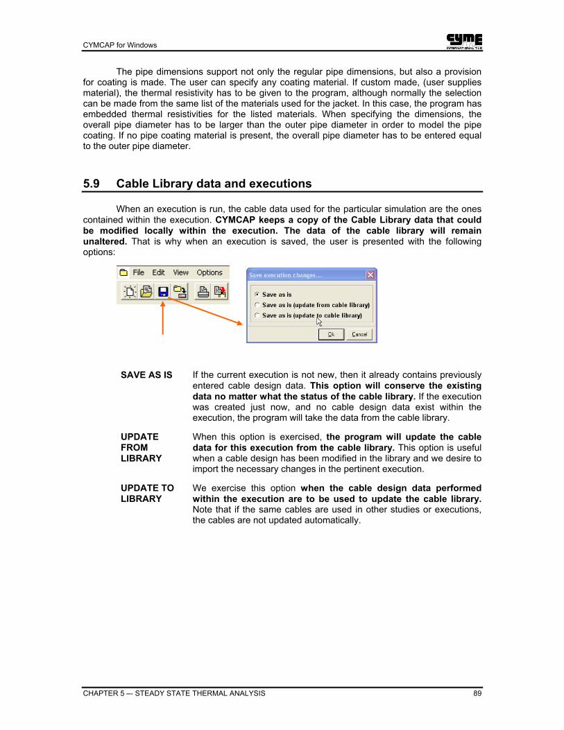
CYMCAP for Windows


The pipe dimensions support not only the regular pipe dimensions, but also a provision for coating is made. The user can specify any coating material. If custom made, (user supplies material), the thermal resistivity has to be given to the program, although normally the selection can be made from the same list of the materials used for the jacket. In this case, the program has embedded thermal resistivities for the listed materials. When specifying the dimensions, the overall pipe diameter has to be larger than the outer pipe diameter in order to model the pipe coating. If no pipe coating material is present, the overall pipe diameter has to be entered equal to the outer pipe diameter.

5.9 Cable Library data and executions

When an execution is run, the cable data used for the particular simulation are the ones contained within the execution. CYMCAP keeps a copy of the Cable Library data that could be modified locally within the execution. The data of the cable library will remain unaltered. That is why when an execution is saved, the user is presented with the following options:

SAVE AS IS If the current execution is not new, then it already contains previously entered cable design data. This option will conserve the existing data no matter what the status of the cable library. If the execution was created just now, and no cable design data exist within the execution, the program will take the data from the cable library.

UPDATE FROM LIBRARY

When this option is exercised, the program will update the cable data for this execution from the cable library. This option is useful when a cable design has been modified in the library and we desire to import the necessary changes in the pertinent execution.

UPDATE TO LIBRARY

We exercise this option when the cable design data performed within the execution are to be used to update the cable library. Note that if the same cables are used in other studies or executions, the cables are not updated automatically.

CYMCAP for Windows


5.10 Steady state thermal analysis, Example 1: Cables in a duct bank

In this study case, the basic steps for setting up a case with cables in a duct bank are illustrated. The cable type to be used is already in the library. If this were not the case the first task would be to create the cable and save it in the library.

The study parameters are as follows:

• Six single-phase cables, composing two 3-phase circuits, located in ducts within a duct bank are considered.

• The cables are 30kV, 1000KCMIL, CU conductor, CU concentric neutral, XLPE insulated cables.

• The duct bank is made of concrete and the cables are assumed to operate at 75% load factor.

• This study will assume that all the cables are of the same type and that are equally loaded.

• The maximum conductor temperature will be assumed to be 90 °C. The frequency will be 60 Hz and the unit system will be the Metric one.

• All 6 cables are of the same type; therefore only 1 cable type will be used for the installation.

The following aspects of CYMCAP are illustrated through this example:

• Defining a new study and a new execution.

• Setting the steady state analysis solution Option.

• Using Execution speed bar and associated command buttons within an execution.

• Utilizing the duct bank library for cables installed in a duct bank, including:

• Defining standard and/or non-standard duct banks.

• Importing a duct bank from the Library .

• Defining the general installation data and setup.

• Defining the cable installation data and entering the geometrical installation data.

• Rearranging the cables in the proper ducts.

• Why it is not necessary to explicitly enter the cables coordinates for duct bank installations.

• How to define specific installation data for the cables within an installation.

• How to generate graphical and tabular reports for a given execution.

• How to access the cable design data graphically from the installation layout.

• How to access graphical reports from the installation layout.

• How to interpret the generated tabular reports for steady state analysis.

CYMCAP for Windows


5.10.1 Defining a new study and a new execution

We enter the CYMCAP Navigator and make certain that the frequency is set to 60 Hz and the Unit system is set to Metric. To change the frequency, double-click on the frequency command in the status bar (Fq=x) and type in the frequency in the dialog box that will be displayed. To change the unit system, double-click on the word Metric or Imperial that appears next to the frequency in the status bar. Double-clicking toggles between the two unit systems.

We then create a brand new study. Click on the New Study button in the Study Navigator page. The program will give you the choice of duplicating the study highlighted in the list to use it as the template (Yes), or not use it and start with a blank study (No). For this example, click No.

CYMCAP for Windows


5.10.2 Setting the steady state analysis solution Option

Click on OK to display the Solution Option dialog box. We select Equally Loaded, since there is only one cable type in the installation and we desire all circuit to have the same ampacity, and click OK.

The program then prompts the user for the generic installation type by displaying the Execution speed bar.

CYMCAP for Windows


5.10.3 Execution speed bar and associated command buttons

Before proceeding, let us examine the contents of the Execution speed bar. This toolbar features the commands that are gateways to important activities within the execution. They also govern the prioritization of data entry and ensuing prompts. The same functions can be accessed from the CYMCAP menu. Depending on whether the execution is a new execution, some (or all) will be enabled. More specifically:

This command is used to invoke the Multiple Duct Banks module (MDB), which is an optional extension to CYMCAP designed to determine the steady state ampacity of cables installed in several neighboring duct banks and/or backfills with different thermal resistivity. The presentation of the remaining of this chapter assumes that the MDB module is not present.

Ductbank – Command part of the generic installation description. It pertains to cables installed within a duct bank. All the cables of the installation must be contained within the duct bank.

Backfill – Command part of the generic installation description. It pertains to the cables installed within a backfill. All the cables of the installation must be contained within the backfill.

Directly buried – Command part of the generic installation description. It pertains to cables installed as directly buried. All the cables of the installation must be directly buried.

Buried ducts – Command part of the generic installation description. It pertains to cables installed in buried ducts. All the cables of the installation must be contained within buried ducts.

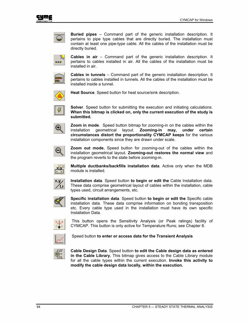
CYMCAP for Windows


Buried pipes – Command part of the generic installation description. It pertains to pipe type cables that are directly buried. The installation must contain at least one pipe-type cable. All the cables of the installation must be directly buried.

Cables in air – Command part of the generic installation description. It pertains to cables installed in air. All the cables of the installation must be installed in air.

Cables in tunnels – Command part of the generic installation description. It pertains to cables installed in tunnels. All the cables of the installation must be installed inside a tunnel.

Heat Source. Speed button for heat source/sink description.

Solver. Speed button for submitting the execution and initiating calculations. When this bitmap is clicked on, only the current execution of the study is submitted.

Zoom in mode. Speed button bitmap for zooming-in on the cables within the installation geometrical layout. Zooming-in may, under certain circumstances distort the proportionality CYMCAP keeps for the various installation components since they are drawn under scale.

Zoom out mode. Speed button for zooming-out of the cables within the installation geometrical layout. Zooming-out restores the normal view and the program reverts to the state before zooming-in.

Multiple ductbanks/backfills installation data. Active only when the MDB module is installed.

Installation data. Speed button to begin or edit the Cable Installation data. These data comprise geometrical layout of cables within the installation, cable types used, circuit arrangements, etc.

Specific installation data. Speed button to begin or edit the Specific cable installation data. These data comprise information on bonding transposition etc. Every cable type used in the installation must have its own specific Installation Data.

This button opens the Sensitivity Analysis (or Peak ratings) facility of CYMCAP. This button is only active for Temperature Runs; see Chapter 8.

Speed button to enter or access data for the Transient Analysis

Cable Design Data. Speed button to edit the Cable design data as entered in the Cable Library. This bitmap gives access to the Cable Library module for all the cable types within the current execution. Invoke this activity to modify the cable design data locally, within the execution.

CYMCAP for Windows


5.10.4 Defining standard and/or non-standard duct banks

Click on the Ductbank installation speed button to call for a duct bank installation. The program displays another prompt to inquire whether a regular duct bank or not is to be used.

Standard duct banks are duct banks featuring symmetrical arrangements of duct rows and columns. Asymmetrical duct banks feature arbitrary duct placement geometry within the duct bank. Click No to indicate that a regular duct bank is to be selected from the Duct bank library.

CYMCAP for Windows


5.10.5 Importing a duct bank from the Library

Once a standard duct bank is selected, the duct bank library becomes accessible, with all its entries in a scroll list. Any duct bank from the library can be selected and brought over. Highlight the desired duct bank in the Library drop down list to import the new duct bank in the installation. It is important at this point to specify the depth at which the duct bank will be placed. Here, the depth is specified by the duct bank center, but the top can also be used to set its location.

CYMCAP for Windows


5.10.6 Defining the general installation data and setup

Click the Apply button at the bottom of the Ductbank Library dialog box to display the Ductbank installation dialog box into which you will enter the General data for the installation (section 5.8.1). The pertinent information is shown below:

Enter your general data and click OK, the program will then display the Installation Setup window.

The following figure illustrates the possible cable configurations. Some options might not be active depending on the type of installation.

This is where you will enter the cables/circuits the installation includes. The simulation under consideration features 6 single core cables, in 2 circuits. The maximum conductor temperature is 90 degrees C and the circuit Load factor 0.75.

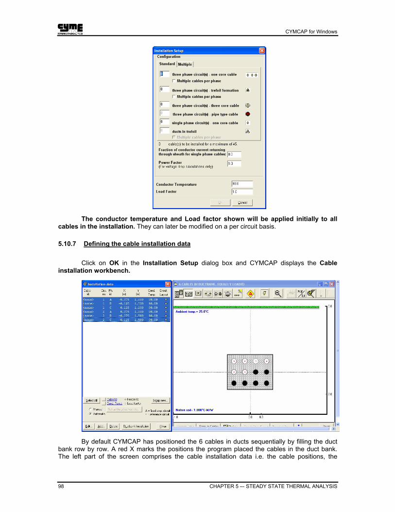
CYMCAP for Windows


The conductor temperature and Load factor shown will be applied initially to all cables in the installation. They can later be modified on a per circuit basis.

5.10.7 Defining the cable installation data

Click on OK in the Installation Setup dialog box and CYMCAP displays the Cable installation workbench.

By default CYMCAP has positioned the 6 cables in ducts sequentially by filling the duct bank row by row. A red X marks the positions the program placed the cables in the duct bank. The left part of the screen comprises the cable installation data i.e. the cable positions, the

CYMCAP for Windows


maximum temperature and the circuit layout. The bitmaps for the circuit layout clearly indicate that we deal with single core cables having one cable per duct.

If other circuit arrangements were chosen different bitmaps would appear for the circuit layout. More specifically:

Single core cable located at the displayed coordinates.

Trefoil formation which center is located at the displayed coordinates.

Three-core cable located at the displayed coordinates.

We need to specify now the cable types that will be used. Position the highlight bar on any cable of the first circuit (or drag it to highlight them all) and double click on it. The Cable library browser replaces the Installation data dialog box.

Selecting any cable type from the library is thus possible, with simultaneous visualization of the cable cross-section within the browser. Furthermore, by activating the Library cable filter the search can be narrowed down to pertinent cables only (e.g. single core). Position the highlight bar on the desired cable and click OK to import it to the installation. Note that CYMCAP will first verify if the selected cable fits in the duct.

Any duct showing an X symbol means that the cable is too large for the conduit.

CYMCAP for Windows


5.10.8 Rearranging the cables in the proper ducts

As seen, the application placed the cable arbitrarily, filling completely the upper row of the duct bank and moving on to the second row sequentially. Most probably this is not the desired cable positioning, then click on the button Permute cables to rearrange the cables as desired by pointing and dragging any cable to the desired location.

Once the desired positioning is achieved, click on the button Apply at the bottom of the

graphical display to accept the changes.

The final position of the cables is shown in the installation screen.

Since the cables in a duct bank installation need to be inside the conduits, CYMCAP can easily find the appropriate location of the cables because the possibilities are finite. In other types of installations this is not possible and the user needs to specify the x, y location of every cable.

CYMCAP for Windows


5.11 A study case for dissimilar directly buried cables

For this example we will consider one trefoil formation of single core cables (350KCMIL, 15kV rated), three single core cables (350KCMIL, 46kV rated submarine cables) in flat formation and one 3-core (250 KCMIL, 69kV rated) cable, directly buried in the ground. The installation therefore features 3 circuits and 3 different types of cables.

The maximum permissible conductor temperatures for the 15kV and 46kV submarine cable circuits shall be assumed to be 90°C, while their respective Load factors are 0.75. The 69 kV circuit will be assumed to have a fixed ampacity of 140.00 A at a load factor of 1.00. An irrigation pipe, having 150 cm diameter is in the vicinity, carrying water. The pipe will be modeled as a heat sink having a temperature of 10°C. The ampacities of the first two circuits are sought. The Unit system will be the Imperial system and the operating frequency shall be assumed to be 60 Hz.

In analyzing this case, the following CYMCAP options are illustrated: • Define a new execution using an existing one as template. • Modify the solution option from the CYMCAP menu. • Enter a group of cables using absolute coordinates. • How to enter in the installation cables using relative coordinates with respect to

already entered cables. • How to enter in the installation cables arranged in a trefoil formation. • How to designate a reference circuit when dissimilar cables are considered for the

installation. • How to perform steady state analysis when one circuit in the installation has a fixed

load carrying capacity. • How to model external heat sources. • How to view the reports for cables arranged in a trefoil formation.

5.11.1 Define a new execution using an existing one as template

We can proceed as in example 1 and define a new study with a new execution in it. An alternative manner is to use the existing execution for duct banks and create a new one within the same study. If the former way is selected, the steps that need to be followed have already been described. If the latter approach is followed, the old installation data need to be deleted and a new installation to be built anew. In both cases the solution option must be specified, in fact changed, to reflect the fact that the installation now has dissimilar cables.

CYMCAP for Windows


5.11.2 Modify the solution option from the CYMCAP menu

The solution Option can be specified from the main CYMCAP Menu. Enter the menu item Edit and access the Solution Option entry.

The new installation will comprise one trefoil formation, one flat formation and one 3-core cable. Since the majority of the conductor temperatures will be 90 °C and most of the circuits will feature a Load factor of 0.75 both can be specified along with the generic circuit description, when defining the installation setup.

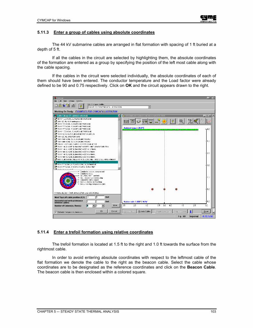
CYMCAP for Windows


5.11.3 Enter a group of cables using absolute coordinates

The 44 kV submarine cables are arranged in flat formation with spacing of 1 ft buried at a depth of 5 ft.

If all the cables in the circuit are selected by highlighting them, the absolute coordinates of the formation are entered as a group by specifying the position of the left most cable along with the cable spacing.

If the cables in the circuit were selected individually, the absolute coordinates of each of them should have been entered. The conductor temperature and the Load factor were already defined to be 90 and 0.75 respectively. Click on OK and the circuit appears drawn to the right.

5.11.4 Enter a trefoil formation using relative coordinates

The trefoil formation is located at 1.5 ft to the right and 1.0 ft towards the surface from the rightmost cable.

In order to avoid entering absolute coordinates with respect to the leftmost cable of the flat formation we denote the cable to the right as the beacon cable. Select the cable whose coordinates are to be designated as the reference coordinates and click on the Beacon Cable. The beacon cable is then enclosed within a colored square.

CYMCAP for Windows


The trefoil formation coordinates are then entered with respect to the beacon cable. As follows:

The last cable (3-core) is entered, using the same cable as beacon cable.

CYMCAP for Windows


5.11.5 Specify a “fixed ampacity circuit”

Click on More to specify the fact that this cable will have a Load factor of 1.00 and that it will be a fixed ampacity circuit. Note that by specifying the circuit to be a reference circuit, the Temperature field reverts to Circuit Ampacity. It is there that the fixed ampacity values need to be entered.

Once the circuits have been defined, since the cables are unequally loaded, one circuit needs to be designated as the reference circuit.

The reference circuit should be the cable circuit containing the hottest cable. If the wrong circuit is selected as reference the program may return “unexpected” results. The hottest cable could have exceeded the specified temperature. This is easily fixed by simply changing the reference to other circuit.

There is the possibility of performing the automatic selection of the reference circuit. This new feature is particularly useful for multiple duct bank installations with many cables when convergence was not obtained to avoid re-constructing the mesh (see next figure). However, the user must check that no target temperatures are being exceeded and that the ampacity of all the circuits is “reasonable”.

CYMCAP for Windows


It has not been made the default for all installations because users of older versions might have gotten the desired results with a specific reference circuit and the automatic selection of reference circuit might yield slightly different results. All new executions could use the automatic selection of the reference circuit.

5.11.6 Convergence and the Selection of Reference Circuit

As mentioned before, the reference circuit should be the circuit containing the hottest cable. CYMCAP converges in most cases when the reference circuit is properly selected. Sometimes, however, it is not easy to estimate before performing the simulation, which circuit would end up being the hottest one. When convergence is not obtained for a particular selection of the reference circuit, the user is encouraged to try all the circuits as reference.

There are a few cases that will not converge even after trying all circuits as reference. To get ampacity results, for at least some of the circuits, the user must change one or more of the circuits to fixed ampacity. This improves the chances for CYMCAP to converge.

Note that convergence only becomes an issue when performing ampacity calculations. Temperature simulations do not need the specification of a reference circuit and the results obtained are always accurate. This feature can be used to get ampacity for those very rare occasions when CYMCAP does not converge for ampacity calculations.

To get ampacity, the user will have to perform a number of temperature simulations varying the specified current of the circuits until the desired operating temperature is obtained. Depending on the number of circuits, a large of number of educated trial-and-error simulations would have to be carried out.

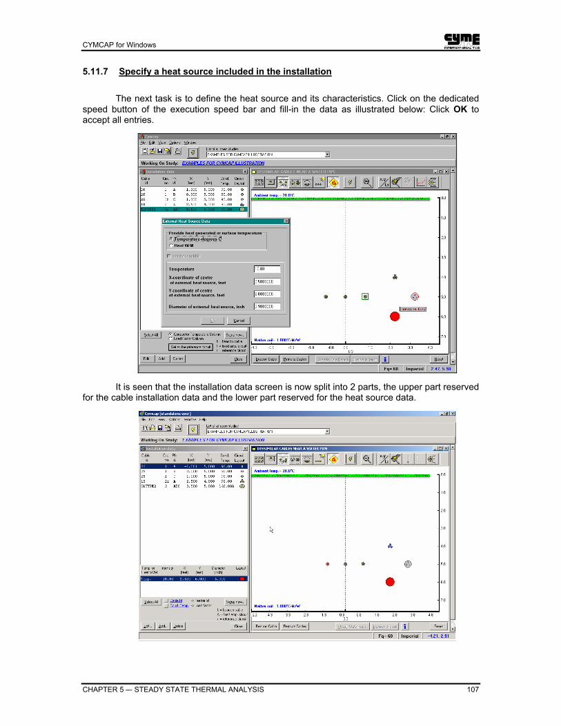
CYMCAP for Windows


5.11.7 Specify a heat source included in the installation

The next task is to define the heat source and its characteristics. Click on the dedicated speed button of the execution speed bar and fill-in the data as illustrated below: Click OK to accept all entries.

It is seen that the installation data screen is now split into 2 parts, the upper part reserved for the cable installation data and the lower part reserved for the heat source data.

CYMCAP for Windows


5.12 Specific installation data

The execution data need now to be completed by entering the specific installation data. The 15kV cables are assumed to be single-point bonded and the 44kV cables two-point bonded, non-transposed with even spacing along the cable run. The 69 kV cable is assumed to be two-point bonded. It is emphasized again that specific installation data need to be entered for all the cable types. The screen below indicates specific installation data for the 46 kV cables arranged in flat formation.

5.13 Results Reporting

CYMCAP has four facilities to report the computed results; three of them are graphical and one tabular (with many discriminating options). The graphical results are shown by:

• Labels directly shown on the installation screen (described in section 5.14 Steady-state results labels)

• Position labels following the mouse selection (section 5.15 Viewing the graphical ampacity reports by mouse selection)

• Combined with option (2) double clicking on the selected cable in the installation will give detailed information on the temperature and losses of a cable per layer.

CYMCAP for Windows


5.14 Steady-state results labels

Steady-State Results Labels have been introduced in CYMCAP to display the steady-state ampacity and temperature results for all cables directly on the installation. This capability allows the user to create enhanced reports using the graphic representation of the installation.

You can position the labels anywhere around the representation of the installation and select the type of connection line the between the individual cables and their associated labels. A label grid can be used also to help you rapidly position all labels orthogonally.

An example of an installation with labels after the solution has been obtained is illustrated below.

CYMCAP for Windows


5.14.1 View/hide labels

The main menu item View includes three options for viewing or hiding the labels. A dot is displayed on the left of the menu command indicating the active option.

No labels Hides all labels on the display. Short cut: CTRL+N All labels Displays all labels. Short cut: CTRL+L Only label(s) with cable(s) selected

Shows only the labels for selected cable(s).

Short cut: CTRL+O

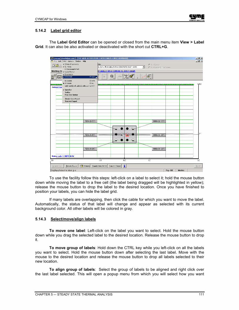
CYMCAP for Windows


5.14.2 Label grid editor

The Label Grid Editor can be opened or closed from the main menu item View > Label Grid. It can also be also activated or deactivated with the short cut CTRL+G.

To use the facility follow this steps: left-click on a label to select it; hold the mouse button down while moving the label to a free cell (the label being dragged will be highlighted in yellow); release the mouse button to drop the label to the desired location. Once you have finished to position your labels, you can hide the label grid.

If many labels are overlapping, then click the cable for which you want to move the label. Automatically, the status of that label will change and appear as selected with its current background color. All other labels will be colored in gray.

5.14.3 Select/move/align labels

To move one label: Left-click on the label you want to select. Hold the mouse button down while you drag the selected label to the desired location. Release the mouse button to drop it.

To move group of labels: Hold down the CTRL key while you left-click on all the labels you want to select. Hold the mouse button down after selecting the last label. Move with the mouse to the desired location and release the mouse button to drop all labels selected to their new location.

To align group of labels: Select the group of labels to be aligned and right click over the last label selected. This will open a popup menu from which you will select how you want

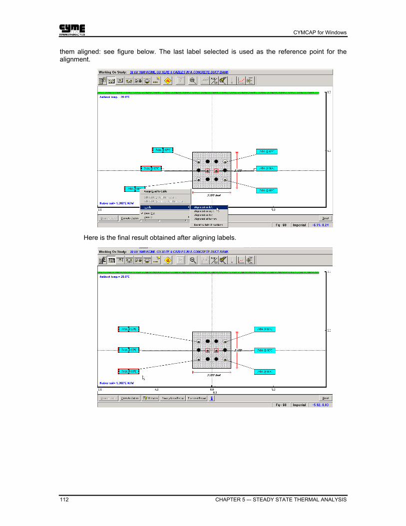
CYMCAP for Windows


them aligned: see figure below. The last label selected is used as the reference point for the alignment.

Here is the final result obtained after aligning labels.

CYMCAP for Windows


5.14.4 Change the connection line between the cable and its associated label

Select any label displayed on the installation and position the mouse cursor over that label. Roll the mouse wheel forward or backward until you find the desired connection line to be used between the cable and the label associated to it. Once done, left click anywhere on the display.

If your mouse does not have a wheel, then go to next sub-section for an alternative way to change the connection line.

5.14.5 Change the properties of a label

Select any label displayed on the installation and double-click to display the Label Editor dialog box to edit the label properties.

The Label Editor dialog box allows you to change the color of a selected label and of its text. You can also change the appearance of the port connector between the cable and the associated label by selecting the picture representing the final look desired. You can apply your selections to all labels by activating the Apply to all labels check box. Once is done, click OK to accept changes.

The figures below show an example of changes applied to one label.

CYMCAP for Windows


5.14.6 Reset all labels to their default positions

After solving an execution, move the mouse anywhere over the graphic representation of the installation and right click to display the popup menu. Open the submenu named Labels and select Reset to default positions. You will be prompted to confirm this action.

You can reset the labels to their default positions at any time.

CYMCAP for Windows


Here is the result obtained after selecting the option.

5.14.7 Keep all labels positions permanently

You simply need to Save the execution to keep the current positions of labels permanently. The next time that this execution will be opened and solved again, all labels will be displayed at the same location as before.

CYMCAP for Windows


5.15 Viewing the graphical ampacity reports by mouse selection

The reports for cables in a trefoil formation follow the same philosophy as for any other cable. The only difference is that CYMCAP recognizes the individual identity of every phase in the trefoil arrangement both when pointing with the mouse on the trefoil arrangement as well as for the detailed reports on a cable per cable basis.

CYMCAP for Windows


If another phase of the trefoil formation is of interest, the scroll list above the bitmap portraying the trefoil gives access to it. Select the appropriate phase and the new report will be generated.

Whenever viewing graphical ampacity reports, the cable that is enclosed in a red square was determined to be the hottest cable in the entire installation.

CYMCAP for Windows


5.16 Tabular Reports

CYMCAP generates a comprehensive steady state report. In addition of displaying the ampacities and temperatures, the steady state tabular report gives also the losses per cable layer, the skin and proximity factors, electrical resistances, thermal resistances per installation layer, standing voltages, and thermal capacitances.

The user gains access to the steady state report after performing a simulation by clicking on the Steady-State Report button at the bottom of the installation screen. When doing so, the following dialog box is displayed.

By clicking on the different radio buttons, the user can discriminate which information is displayed in the bottom part of the dialog box. The entire report, or sections of it, can be printed or saved into a file. Please be advised that the information in the steady state report is not saved in the CYMCAP database and when the execution is closed or changed, the information is lost. It will be necessary to re-run the execution to visualize it again.

5.17 MS Excel (Final) Report

CYMCAP (version 4.3 and higher) generates an extended graphical/tabular report in MS Excel format. It is intended as a final report that can be produced when the user is satisfied with the results and he/she wishes to write a report. To gain access to it click on the Excel Report button (as shown in the figure).

The Excel report will at the very least produce the summary report. It includes all the general input data, a figure with the installation and a table with the ampacity per cable. Depending on the number of cables and the installation type, the report may be in one or two pages. The following figures show and example.

The Summary report may include your company’s logo. For this, it will be necessary to capture the logo and enter it into the file Logo.jpg. The file should be set on the directory where CYMCAP is installed. The logo will be placed in the upper right-hand side corner (see figure below).

The Summary tab of the Excel sheet is always produced. When the user is working with the Imperial system of units this is the sole tab that will be produced. When the user wants the extended report, it is necessary to work in the Metric system of units.

CYMCAP for Windows


You can now operate on the results using the tools available in Excel; you can save or print the report as you wish. There are no facilities to automatically close Excel, thus the user will have to close it manually.

CYMCAP for Windows


When the user is working with the Metric system of units, the Excel report may contain up to 5 working sheets. Depending on the selected solution options and the modules that the user is subscribed to, the following reports could be generated:

• Summary – As described above.

• Electrical – Containing important electrical parameters, such as: resistances, inductances, capacitances, sequence impedances, losses, voltage drop, etc.

• Steady State – Displaying all intermediate calculation for the steady state ratings in accordance to the IEC 60287 Standards.

• Emergency – Duplicating the hand calculation of the emergency cable rating methods given in the IEC 60853 Standards.

• Short Circuit – Displaying all the parameters used in the IEC Standard 60949 for short circuit rating (only if the user has subscribed to the SCR module).

The following figure shows how the information is classified in the Excel reports. As before the user is free to operate, save and print one or all the sheets of the enhanced report.

CYMCAP for Windows


5.17.1 The Electrical Tab

The electrical tab requires further explanation and clarification. The displayed parameters have been computed with simplified equations and the user should use them in an informed manner and only when he/she is in full agreement with the calculation method. The equations and meaning of each parameter for the quantities not available in the IEC Standards 60287 are described next.

Dielectric Stress at conductor surface

=

i

ei D

DD

U

ln21

Stress Dielectric 0 [kV/mm]

Where: U0 = Phase to Neutral Voltage [kV] Di = Internal diameter of insulation (excluding shield) [mm] De = External diameter of insulation (excluding screen) [mm]

Inductance of Conductor

+=

cDS

KL2

ln2.0 [mH/km]

Where: S = Axial spacing between the conductors [mm] Refer to IEC 60287-1-1 (Clauses 2.3) Dc = Conductor diameter [mm] K = 0.0642 (for 7 wires stranded conductor) = 0.0554 (for 19 wires stranded conductor) = 0.0528 (for 37 wires stranded conductor) = 0.0514 (for 61 wires and above stranded conductor) = 0.05 (for solid conductor)

Reactance of Conductor

10002 Lf

Xπ

= [Ω/km]

Where: L = Inductance (mH/km) f = Frequency [Hz]

Positive Sequence Impedance

XjRZ Cac +=+ o90_ [Ω/km]

Negative Sequence Impedance

XjRZZ Cac +== +− o90_ [Ω/km]

CYMCAP for Windows


Zero Sequence Impedance

000 XjRZ += [Ω/km]

Where: R0 = Zero sequence resistance of the conductors per phase = AC Resistance of one conductor @ 20 °C without the increase for proximity effect + 3 resistance of the metallic covering for 3 core cables or + the resistance of the metallic covering for single core cables or + the resistance of one metallic sheath in parallel with three times the resistance of the armor for SL cables X0 = Zero Sequence Reactance = Reactance of sheath (see below)

Inductance of Sheath (and Concentric Wires)

=dSLs 2ln2.0 [mH/km]

Where: S = Axial spacing between the conductors [mm] Refer to IEC 60287-1-1 (Clauses 2.3) d = the mean diameter of the sheath [mm]

Reactance of Sheath

10002 LsfXs π

= [Ω/km]

Insulation Resistance @ 20 °C

=

i

eDDCIR ln

2100020@

πo [MΩ.km]

Where: Di = Internal diameter of insulation (excluding shield) [mm] De = External diameter of insulation (excluding screen) [mm]

Insulation Resistance @ 90 °C

10020@90@ CIRCIR

oo = [MΩ.km]

Capacitance

=

i

eDD

Cln18

ε [mF/km]

Where: Di = Internal diameter of insulation (excluding shield) [mm] De = External diameter of insulation (excluding screen) [mm] ε = Relative Permittivity of insulation Refer to IEC 60287-1-1 (Clause 2.2)

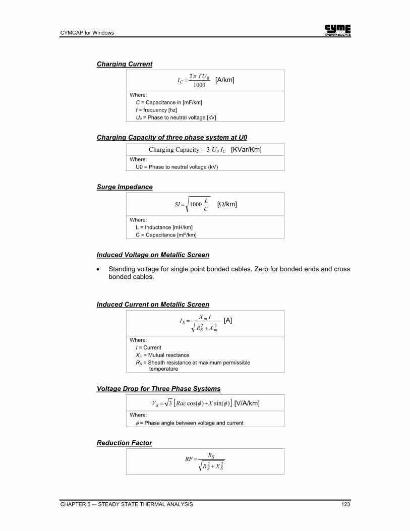
CYMCAP for Windows


Charging Current

10002 0UfIC

π= [A/km]

Where: C = Capacitance in [mF/km] f = frequency [hz] U0 = Phase to neutral voltage [kV]

Charging Capacity of three phase system at U0

Charging Capacity = 3 U0 IC [KVar/Km] Where:

U0 = Phase to neutral voltage (kV)

Surge Impedance

CLSI 1000= [Ω/km]

Where: L = Inductance [mH/km] C = Capacitance [mF/km]

Induced Voltage on Metallic Screen

• Standing voltage for single point bonded cables. Zero for bonded ends and cross bonded cables.

Induced Current on Metallic Screen

22mS

mS

XR

IXI+

= [A]

Where: I = Current Xm = Mutual reactance RS = Sheath resistance at maximum permissible temperature

Voltage Drop for Three Phase Systems

[ ])sin()cos(3 φφ XRacVd += [V/A/km]

Where: φ = Phase angle between voltage and current

Reduction Factor

22SS

S

XR

RRF+

=

CYMCAP for Windows


5.18 Opening more than one executions simultaneously

CYMCAP offers the possibility to work simultaneously on more than one execution. The executions may belong to the same or to different studies. In order to be able to open more than one execution, the CYMCAP Navigator needs to remain accessible. Once the navigator appears, click on the Hide on Edit checkbox to remove the tick mark. By default, the tick-mark is on, instructing CYMCAP to close the Navigator when an execution is edited. This is because the program assumes by default that the user will work on one execution at the time. If the tick-mark is removed, then the Navigator stays on to edit another execution when the previous execution has already been edited.

Note that the execution title appears at the top of the screen. There is also a scroll-list that contains the names of all the studies opened. The study title also appears clearly above the CYMCAP ribbon. If a second execution is opened, from the same study, the active windows will show the second execution unless CYMCAP is instructed to either tile or cascade the Windows (access the menu entry Windows to set the desired Option). Cascaded, the two executions look as follows.

CYMCAP for Windows


The windows highlighted pertain to the execution that was loaded last. Note that the

same could have been accomplished by clicking on the study title alone. In that case, all the executions within the study will be opened automatically.

CYMCAP groups the edited executions by study in order to facilitate editing. If the executions for one study are already opened and another study is opened, the executions for the previous study are iconized and the executions of the new study appear cascaded in the foreground. The newly opened study is added to the study scroll list. By accessing the proper study on the scroll-list one can bring to the foreground all its executions and iconize the rest without having to close individually all the executions in the foreground.

CYMCAP for Windows


If any of the executions in the foreground are closed, the remaining ones from the study are available. If all the executions within the study are closed, then all the iconized executions will appear in the foreground.

The same principles apply when editing executions from different studies and there is only one execution per study.

CYMCAP for Windows


5.19 Working with more than one executions simultaneously

Once more than one execution is opened any one can be designated as active. The following screen portrays two executions tiled vertically.

By performing any type of editing or operation, the execution occupies completely the

foreground as if it as the only one opened. The executions remain independent each retaining its own ribbon with full access to the entire editing facilities.

5.19.1 Submitting more than one executions simultaneously

Once 2 (or more) executions are opened, they can be submitted individually by clicking

on the Solve all executions button located next to the CYMCAP ribbon. All the reports for both executions will be generated.

CYMCAP for Windows

CHAPTER 6 –- TRANSIENT ANALYSIS 129

Chapter 6 Transient Analysis

6.1 General

Transient thermal analysis is performed to assess the maximum permissible currents that a cable can sustain over a specific period of time without violating cable material thermal specifications. These violations could either lead to imminent cable failure or substantially shorten the cable's life by causing premature failure. The transient analysis options supported by CYMCAP addresses these concerns and are subsequently analyzed.

6.2 Preliminary considerations

Transient analyses can only be performed after a steady state thermal analysis for the installation has already been successfully performed. This is because a part of the steady state simulation results are used as initial conditions for the transient calculations.

Every cable in the installation must be assigned a load curve for transient analysis studies. This curve determines the variation of the current over a given period of time. The actual ampacity assigned to the cable under transient conditions, is determined with the aid of the SCALING FACTOR. This number is a factor by which the steady state cable current, as resulted from steady state analysis, will be multiplied. The load curve itself has also a factor of its own for every portion in the curve (see Chapter 4). Therefore the current applied to the cable, for a given time interval, will be the product of the cable current as resulted from steady state analysis multiplied by the effective load curve scaling factor.

Note that the program does not support transient calculations in the presence of moisture migration. This means that transient studies can only be executed for the cases where moisture migration was not modeled in steady state. No transients for cables installed in air and/or riser poles, are supported either.

CYMCAP for Windows

130 CHAPTER 6 –- TRANSIENT ANALYSIS

6.3 Transient analysis options

6.3.1 Solve for Ampacity Given Time and Temperature

In this analysis option, the user enters the temperature that a specific cable component (conductor, sheath, etc.) is to reach in a desired time (hours) and the program computes the maximum possible current for the cables. The same cable component is effective for all cables in the installation. The user should NOT select a temperature below the ambient temperature used for the steady state analysis. The following screen illustrates the parameters involved.

Since more than one circuit may be present in the installation, it may be desirable to determine the ampacity of some with the remaining at a constant current value. This is expressed by the notion of the “participating circuit”. The program will calculate ampacities for all “participating” circuits if the option “simultaneously” is selected. Instead, if the option “one at a time” is selected, the program will calculate ampacities for one circuit at a time assuming that the remaining are held at their steady state loading. Non-participating circuits are always held at their steady state loading.

The program reports the required cable currents in terms of SCALING FACTORS based on the results obtained form the steady state analysis.

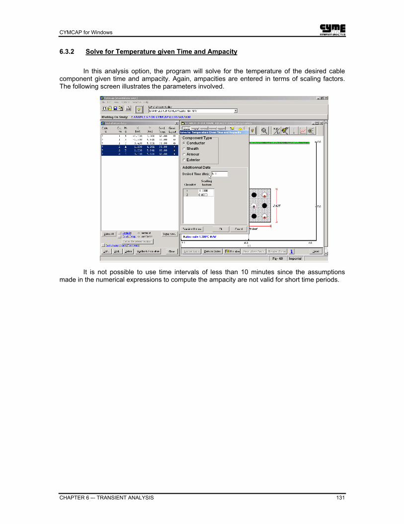
CYMCAP for Windows


6.3.2 Solve for Temperature given Time and Ampacity

In this analysis option, the program will solve for the temperature of the desired cable component given time and ampacity. Again, ampacities are entered in terms of scaling factors. The following screen illustrates the parameters involved.

It is not possible to use time intervals of less than 10 minutes since the assumptions made in the numerical expressions to compute the ampacity are not valid for short time periods.

CYMCAP for Windows


6.3.3 Solve for Time given Ampacity and Temperature

In this analysis option the user specifies the maximum temperature of the component of interest and the current. The program will calculate the time required to reach these conditions for the first time. When step-loading functions are applied, the program will calculate the time at which the maximum permissible temperature is reached. When more complex loading patterns are considered, the program will calculate only the FIRST occurrence (in the specified range) of the user-specified value of temperature and scale factor. The following illustrates the parameters involved.

Both the accuracy and the solution speed depend upon the selected RANGE OF SEARCH TIME and RESOLUTION. There are cases for which the program may not be able to find a solution. In this case, verify that the time range dictated for the search is consistent with the temperatures and ampacities specified.

CYMCAP for Windows


6.3.4 Ampacity as a function of Temperature

This option is similar to the second option described earlier with the difference that instead of considering one ampacity (scale factor) the program considers many at the time. The user supplies, as before, the cable component of interest (conductor sheath etc.), the required time of analysis in hours and a set of scaling factors. The set of scaling factors is defined by specifying the INITIAL and FINAL value for the scaling factor range and the RESOLUTION of the scale factor interval. The following illustrates the parameters involved.

For each scale factor there will be a different ampacity and therefore a different temperature the component of interest will reach in the specified time. The notion of “participating’ circuits” becomes relevant here as well. By default, all circuits are considered as “participating” unless a scaling factor is specified.

6.3.5 Ampacity as a function of Time

This option is similar to the third option described earlier with the difference that instead of considering one ampacity (scale factor) the program can consider many. The user supplies, as before, the cable component of interest (conductor, sheath, etc.) and the maximum permissible temperature that the component can reach. The program will then calculate how long the cables can carry a given set of currents.

The loads of interest are defined by specifying an INITIAL and a FINAL value for the scale factor as well as a RESOLUTION. This option requires the user to supply a time interval within which the calculations are made. It is possible that for a given set of data no solution will be found in the specified time interval.

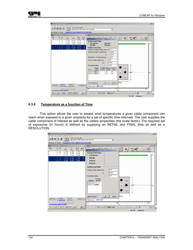
CYMCAP for Windows


6.3.6 Temperature as a function of Time

This option allows the user to assess what temperatures a given cable component can reach when exposed to a given ampacity for a set of specific time intervals. The user supplies the cable component of interest as well as the cables ampacities (the scale factor). The required set of exposures (in hours) is defined by supplying an INITIAL and FINAL time as well as a RESOLUTION.

CYMCAP for Windows


6.4 How to proceed for a transient analysis

The following steps are normally followed in the indicated sequence in order to carry out any of the transient analysis options.

1. Make sure that the load curves to be used are in the load curve library. If not, enter them first and then proceed.

2. Choose the appropriate transient analysis option and provide all the necessary data.

3. Assign loads to cables. This activity is crucial because it is here that the specific load curves will be assigned to various cables.

4. Save the changes for the new execution.

5. Submit the desired execution to obtain the steady state results and transient analysis.

6. View tabular and graphical results.

6.5 Informing CYMCAP that a transient analysis is to be performed

Suppose that for an existing execution a transient analysis is to be performed. Edit the execution at hand. Then from the CYMCAP menu select the Edit > Solution Option > Transient Analysis menu option. The check mark that appears next to it is the flag that indicated to CYMCAP that a transient simulation is to follow the steady state analysis.

CYMCAP for Windows


6.6 Example and Illustrations

6.6.1 Case description and illustrations

During the following example, the execution analyzed in chapter 6, featuring 6 cables in a duct bank is used to illustrate the process of performing a transient analysis with CYMCAP. Temperatures of all cables as function of time will be generated. Every circuit shall be assigned a different Load and the conductor temperatures as a function of time will be assessed. The Load curve for circuit 2 shall be considered to be the same as the Load curve for circuit 1. An overload of 20% and 40% will be assumed for the circuits #1 and #2 respectively. The temperatures will be monitored for 48 hours.

During the course of this example the following aspects of CYMCAP are illustrated:

• Specify the transient analysis option.

• Specify the data for the transient analysis option.

• Assign Loads to Cables.

• Submit the simulation.

• Generate the reports and view tabular and graphical results for transient analysis.

• How to selectively display results for various cables in the installation

• Change the color of the curves for the transient reports.

• Trace the transients results with the mouse instead of generating tabular reports.

CYMCAP for Windows


6.6.2 Specify the transient analysis option

Edit the execution, and as described in the previous paragraph, enable the transient analysis option. Then click on the ribbon bitmap that gives access to the transient data to select the desired analysis option.

6.6.3 Specify the data for the transient analysis option

Once the desired transient option has been selected, we need to provide the accompanying data.

Click on OK to accept the data and let us now assign loads to cables.

CYMCAP for Windows


6.6.4 Assign Loads to Cables

Click on the button labeled “Go to assign loads (transient)” located at the bottom left of the installation window (the same function can be performed by right clicking anywhere on the window that contains the pictorial representation of the cable installation.

The Load Curve library window is then displayed and any load curve can be assigned to the circuit in question. For this particular example the “weekly” loading curve will be used. Highlight the desired Load curve and click the Apply button. The same operation is repeated for the second circuit.

CYMCAP for Windows


6.6.5 Submit the simulation

Once the transient data is entered, the execution is submitted by clicking on the appropriate NAME on the ribbon. Although, this is the same button as used for steady state analysis, the transient analysis follows for this case. The successful completion of both steady state and transient analysis is indicated.

Once both steady state and transient analyses are successful, reports for both are available as the enabled buttons at the bottom of the screen indicate. Both reports can be accessed through these buttons.

CYMCAP for Windows


6.6.6 Generate the reports

Click on the Transient report button and, by default, the results for the first circuit appear.

The cables for which graphical results are displayed, are also color-highlighted on the actual installation and on the Installation Data dialog box to the left. Results for any cable in the installation can be selected by either (a) highlighting the cable on the cable installation screen (left) portraying the cables coordinates (b) pointing to the cable of interest in the installation and clicking on it. In either case, the cables are highlighted for clarity.

The horizontal dashed line shown on the graph represents the maximum permissible temperature specified in the data. Click on the Select All button at the bottom of the Installation Data dialog box to view the graphical results for all the cables. Similarly, any phase can also be viewed alone by highlighting it.

The load curve associated with any circuit can be superimposed on the graph picturing the temperature variations with time by clicking on the dedicated bitmap of the transient report window as illustrated below.

CYMCAP for Windows


Furthermore, a tabular report is available that portrays the time intervals during which the stipulated maximum temperature has been exceeded. Again, this can be accomplished by clicking on the dedicated bitmap in the ribbon of the transient report window. The result for this particular case, (no such intervals exist) is illustrated below:

CYMCAP for Windows


6.6.7 Change the color of the curves for the transient reports

It is also seen that the graphical results window indicates what cable and what phase is drawn. The color can be changed by double clicking on the color indicator of the curves.

6.6.8 Trace the transients results with the mouse

The results for the transient simulation can be graphically traced with the mouse. Position the mouse anywhere on any curve generated and an ordered pair appearing at the bottom right indicates what temperature pertains to what time.

CYMCAP for Windows


Finally, tabular reports are also available for the transient analysis. Both tabular and graphical reports can be printed/plotted and copied to the Windows clipboard as the appropriate bitmaps within the report-Windows indicate. Tabular reports can be generated by clicking on the most-left bitmap of the transient report window ribbon.

CYMCAP for Windows

CHAPTER 7 –- APPROXIMATE TEMPERATURE FIELD 145

Chapter 7 Approximate Temperature Field

7.1 Introduction

After a successful steady state simulation, CYMCAP can plot an approximate map of the isotherms for underground installations. The easiest way to produce the plot is by clicking on Ctrl–t. Alternatively, the plot can be obtained using the View→Approximate Temperature Field menu option.

CYMCAP for Windows

146 CHAPTER 7 –- APPROXIMATE TEMPERATURE FIELD

7.2 Scopes and Limitations

There are important assumptions made in the calculation of the temperature distribution. The user needs to be aware that CYMCAP only displays an approximate plot of the isothermals. As a consequence of the assumptions, the temperature values are only accurate at a far distance from the cables and when they are directly buried in soil with uniform and constant thermal resistivity.

The assumptions are the following:

• All media is assumed isotropic, homogeneous and linear. Therefore, air inside ducts and pipes is not considered. The concrete of backfills and duct banks is also neglected.

• Heat sources are represented as filaments

• The image method is used to warrant an isothermal (at ambient temperature) at the soil-air boundary

r'

r

h

h

surface

p(x,y)

θambient

Under those conditions we can compute the temperature with the fundamental solution of Fourier Law. This is obtained next. Let us start with the general expression of Fourier Law:

Wρθ −=∇2

Where: θ = Temperature [°K] ρ = Soil thermal resistivity [°K-m/W] W = Heat loss [W/m]

In cylindrical coordinates and assuming that there is not longitudinal heat flow (consistent with CYMCAP calculations) we have:

0)(1)(2

2=++ Wr

drd

rr

drd ρθθ

The fundamental solution is given by:

+=rrWr ambient'ln

2)(

πρθθ

Adding the effect of all conductors (and their images) we get (in Cartesian coordinates):

∑=

−+−

++−+=

conductorsN

k kk

kkkambient

yyxx

yyxxWyx

122

22

)()(

)()(ln

2),(

πρθθ

CYMCAP for Windows


7.3 Customizing the Isotherms

The number, level, color and value labels of the isotherms can be customized. After a successful steady state simulation, the users can gain access to the customization facility clicking on:

The defaults are shown in the next figure:

CYMCAP for Windows


The color of an individual isotherm is changed by double clicking on the color line and selecting a new one from the palette (see figure below).

A single value or a range can be added. Adding a range between 40 and 50 with a step of 2 is illustrated below.

The resolution the number of numerical labels and the zoom can be adjusted from the lower part of the Contour level data screen.

CYMCAP for Windows


The defaults produce acceptable results in most cases for isotherms that are not very close to the cables, which are the more accurate ones. Isotherms that are close to the cable may appear broken. This can be easily fixed by reducing the resolution. When the resolution is too small the calculation time could be very large. After 10 seconds the following message is issued.

7.4 Automatic Design of Backfills/Duct Banks

One of the applications of the approximate temperature field plot is the ability to determine the size of a backfill or duct bank. For example, consider that moisture migration will be prevented by substituting the native soil with temperature above 60°C by a backfill of thermally stable material. Start by performing a directly buried steady state ampacity simulation. Then press Ctrl-t to produce the temperature field plot.

Frequently it is necessary to zoom out to be able to see the bottom part of the installation.

Then by clicking and dragging the mouse from one corner to another the selected rectangular area can become automatically a backfill; see the figure.

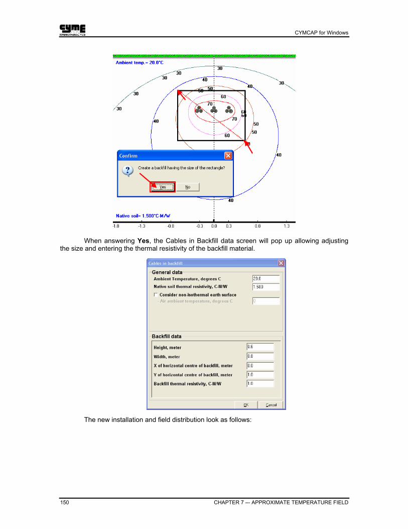
CYMCAP for Windows


When answering Yes, the Cables in Backfill data screen will pop up allowing adjusting the size and entering the thermal resistivity of the backfill material.

The new installation and field distribution look as follows:

CYMCAP for Windows


Remember that in the temperature field plot the presence of backfills and ducts is neglected.

If you do not like your results and need a different size you can simply click and pull to create a different size backfill (see figure below).

CYMCAP for Windows


This functionality works for:

• Directly buried • Backfills • Buried ducts • Nonstandard duct banks

CYMCAP for Windows

CHAPTER 8 –- THE SENSITIVITY ANALYSIS OPTION OF CYMCAP 153

Chapter 8 The Sensitivity Analysis Option of CYMCAP

This activity permits a particular kind of sensitivity analysis and is implemented to automate the generation and solution of a particular set of executions pertaining to the so-called “Peak Ratings Analysis”.

The problem manifests itself, normally, for various circuits (feeders) within a duct bank and can be defined as follows:

• Assume that the installation has a certain number of circuits.

• Assume that the “Temperature” analysis Option is selected for the steady state analysis. That means that for all involved circuits, currents are impressed and resulting temperatures as sought. This is considered to be the base case for the analysis.

• Assume now that one is interested in finding the maximum current that can be impressed in any of the circuits so that its temperature does not exceed a target temperature while the rest of the circuits remain unaltered, i.e., they carry the same currents as in the base case.

• Assume that the same question is of interest for all the circuits within the installation, considered one at a time.

If this problem is to be resolved using the base facilities of the program the user will be forced to:

• Create a new execution every time a new circuit is to be examined.

• For every one of these executions, the circuit in question needs to be selected.

• The circuit current needs to be changed to limiting temperature instead.

• The solution Option needs to be changed to “Unequally Loaded”

• The circuit in question needs to be labeled as the “Reference circuit”

• The execution needs to be renamed and saved

• The process needs to be repeated for all involved circuits.

• All the executions need to be submitted for solution.

All these activities are permissible activities and perfectly well defined within the capabilities of the program. The fact, however, remains that this is a tedious process and prone to error. That is why the Sensitivity Analysis option at hand is implemented to fully automate the process. In other words, the program will automatically generate the needed executions with the proper configuration, solve them simultaneously without any unnecessary user intervention and display the reports in a manner conducive to ready inspection. Furthermore, more than one limiting temperature can be requested on a per circuit basis.

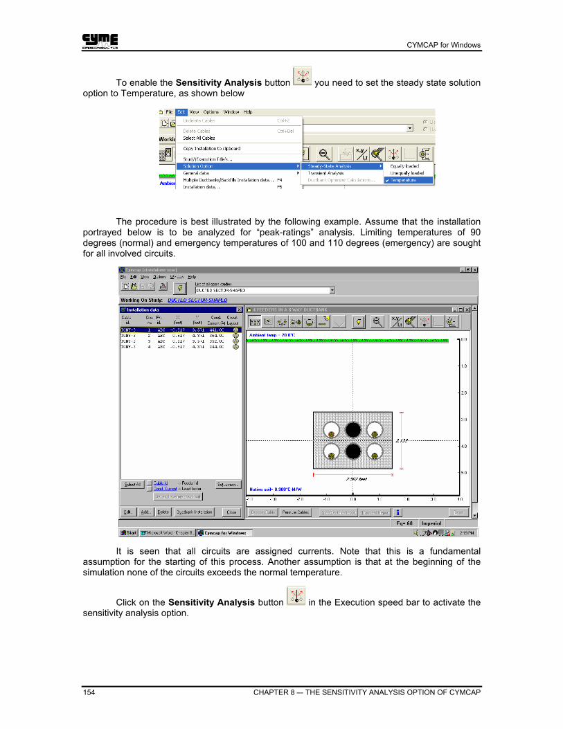
CYMCAP for Windows

154 CHAPTER 8 –- THE SENSITIVITY ANALYSIS OPTION OF CYMCAP

To enable the Sensitivity Analysis button you need to set the steady state solution option to Temperature, as shown below

The procedure is best illustrated by the following example. Assume that the installation portrayed below is to be analyzed for “peak-ratings” analysis. Limiting temperatures of 90 degrees (normal) and emergency temperatures of 100 and 110 degrees (emergency) are sought for all involved circuits.

It is seen that all circuits are assigned currents. Note that this is a fundamental assumption for the starting of this process. Another assumption is that at the beginning of the simulation none of the circuits exceeds the normal temperature.

Click on the Sensitivity Analysis button in the Execution speed bar to activate the sensitivity analysis option.

CYMCAP for Windows

CHAPTER 8 –- THE SENSITIVITY ANALYSIS OPTION OF CYMCAP 155

For this particular case, two emergency temperatures were requested (100 and 110 degrees) because the step was chosen to be 10.0 degrees. Since there are four circuits in the installation, a total of twelve executions shall be created (one execution for the normal temperature of 90 degrees and two for the emergency temperatures of 100 and 110 degrees for every circuit). Once the execution is saved, the ensuing prompt requests confirmation of the activity.

Click Yes to Proceed, and a total of 12 executions are created as can be seen in the Study Navigator.

CYMCAP for Windows

156 CHAPTER 8 –- THE SENSITIVITY ANALYSIS OPTION OF CYMCAP

These executions are already tagged and appear below the “parent” execution, featuring only currents in the circuits.

These executions need to be edited and solved. Click the Edit tagged button in the Navigator to display each in its dedicated window. All the windows will be arranged in cascade.

The Solve All Execution button in the CYMCAP toolbar can be used to solve them all simultaneously and results can be viewed at will after that.

CYMCAP for Windows

CHAPTER 9 –- THE CYMCAP MENU 157

Chapter 9 The CYMCAP Menu

9.1 Overview of the CYMCAP Menu

When outlining the program operational aspects in previous chapters, the application was operated from the Execution speed bar. Many of these functions can also be accessed from the CYMCAP menu located at the top of the screen encompassing the opened execution(s). The initial description assumes that CYMCAP was activated and that the Navigator is closed.

The CYMCAP menu features Files, Window, Help

9.2 The Files menu

Click on the Files menu and the options to either open a New study, Open Navigator or Exit appear as alternatives.

The first two menu options are also accessed through buttons located below the main menu items.

Open a new study

Display the CYMCAP Navigator (or pressing the F3 key)

CYMCAP for Windows

158 CHAPTER 9 –- THE CYMCAP MENU

9.3 The Windows menu

The Windows menu allows managing how executions will appear on the screen, if more than one were opened.

By default, executions will be displayed in Cascade.

9.4 The CYMCAP menu for opened executions

Once an execution is opened, the CYMCAP menu is expanded to accommodate the execution-related activities.

The menu items are File, Edit, View, Window and Help.

9.5 The File menu - Execution

By accessing now the CYMCAP menu item “File” it is seen that the previously displayed menu is expanded with execution management options.

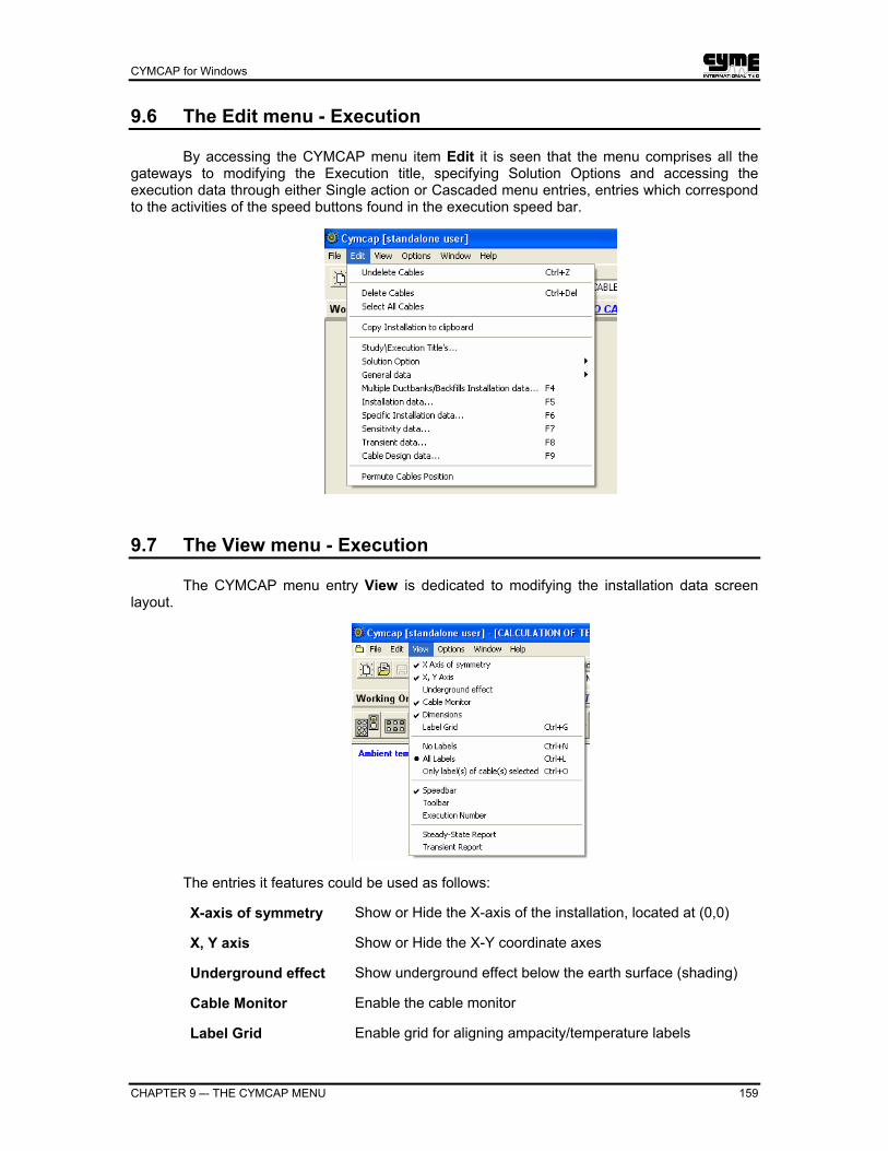
CYMCAP for Windows


9.6 The Edit menu - Execution

By accessing the CYMCAP menu item Edit it is seen that the menu comprises all the gateways to modifying the Execution title, specifying Solution Options and accessing the execution data through either Single action or Cascaded menu entries, entries which correspond to the activities of the speed buttons found in the execution speed bar.

9.7 The View menu - Execution

The CYMCAP menu entry View is dedicated to modifying the installation data screen layout.

The entries it features could be used as follows:

X-axis of symmetry Show or Hide the X-axis of the installation, located at (0,0)

X, Y axis Show or Hide the X-Y coordinate axes

Underground effect Show underground effect below the earth surface (shading)

Cable Monitor Enable the cable monitor

Label Grid Enable grid for aligning ampacity/temperature labels

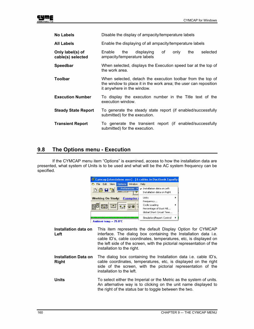
CYMCAP for Windows


No Labels Disable the display of ampacity/temperature labels

All Labels Enable the displaying of all ampacity/temperature labels

Only label(s) of cable(s) selected

Enable the displaying of only the selected ampacity/temperature labels

Speedbar When selected, displays the Execution speed bar at the top of the work area.

Toolbar When selected, detach the execution toolbar from the top of the window to place it in the work area; the user can reposition it anywhere in the window.

Execution Number To display the execution number in the Title text of the execution window.

Steady State Report To generate the steady state report (if enabled/successfully submitted) for the execution.

Transient Report To generate the transient report (if enabled/successfully submitted) for the execution.

9.8 The Options menu - Execution

If the CYMCAP menu item “Options” is examined, access to how the installation data are presented, what system of Units is to be used and what will be the AC system frequency can be specified.

Installation data on Left

This item represents the default Display Option for CYMCAP interface. The dialog box containing the Installation data i.e. cable ID’s, cable coordinates, temperatures, etc, is displayed on the left side of the screen, with the pictorial representation of the installation to the right.

Installation Data on Right

The dialog box containing the Installation data i.e. cable ID’s, cable coordinates, temperatures, etc, is displayed on the right side of the screen, with the pictorial representation of the installation to the left.

Units To select either the Imperial or the Metric as the system of units. An alternative way is to clicking on the unit name displayed to the right of the status bar to toggle between the two.

CYMCAP for Windows


Frequency To select any system AC electrical frequency for the thermal studies. An alternative way to achieve the same is by clicking on Fq= displayed to the right of the status bar to display the dialog box.

Cyclic Loading To select particular option for Cyclic Loading. The Neher-McGrath approach is the default.

Percentage of Duct Fill

To select the duct fill permitted for the ducted cables.

If 100% duct- fill is assumed, the program will verify the total external diameter of the cable, or the equivalent of a trefoil arrangement, with the internal diameter of the duct prior to permitting the placement of any cable in the duct. If another duct-fill percentage is specified, the program will compare the total external diameter of the cable with the internal duct diameter multiplied by the duct-fill factor. This is a precaution taken due to the fact that some margin is normally required between the duct and the cable so that the latter can be pulled in the duct.

The duct-fill factor can therefore determine whether a cable is eligible to be positioned within a given duct or not, during the editing process of the installation. Note that the program will ignore any inconsistencies and/or violations if the duct-fill factor is modified after the data has already been entered.

CYMCAP for Windows


Simulation/Report Control – Steady State

To select important simulation control parameters and the generation of a simulation Control report. These facilities are provided for the eventuality the numerical solution algorithm does not converge.

Simulation/Report Control – Transient Analysis

In general users do not have access to this option. These facilities are provided for advanced users, and only upon request, to better control the transient simulation process.

9.8.1 Simulation control parameters

• Convergence can be facilitated by relaxing (increasing) either the current or temperature convergence tolerance thresholds. These thresholds are, by default for steady state established to 1 A and 0.1 °C respectively. For Transients the tolerance is set to 0.5 °C. If increased, the program may converge for more cases at the expense of a less accurate solution. Still, generally a good estimate of the expected currents is obtained.

• The iteration report can be generated in order to view at what point the iterative procedure starts diverging. Quite often, the divergence manifests itself very close to the solution so once again a very good estimate of the expected currents can also be obtained through the iteration report.

• The number of iterations can also be increased/decreased at will. Experience with the program has however shown that 100 iterations are more than sufficient for steady state and 50 for transients. In fact, the program normally converges in less than 10 iterations.

• Unless valid reasons exist for modifying them it is strongly recommended that the simulation parameters control settings be left at their default values.

CYMCAP for Windows


9.9 Designate the Unit System for the session

CYMCAP permits the utilization of either the Metric or the Imperial system of units in order to facilitate data entry and avoid unnecessary conversions that otherwise would have to be done by the user. North American practice is still geared towards the Imperial system of units, while European and International practice favors the Metric System.

When the Imperial system of units is used, cable dimension and related data must be entered in KCMIL and inches while cable installation geometrical data must be entered in feet. For the Metric system, cable dimensions and related data are entered in mm and cable installation geometrical data in meters. In order to designate the system of units, activate the program and when the CYMCAP navigator comes up on screen, point to the status bar where the word (or Imperial) appear and click on it. This is a toggle switch that reverts to the alternative system of Units.

Note that during the simulation, the program permits to switch the system of units thus assuring even greater flexibility.

9.10 Designate the AC system frequency for the session

The ac system frequency is an important parameter in ampacity calculations for power cables in alternating current installations. Dielectric losses, ac conductor resistance and other important parameters are a direct function of the system frequency. In order to designate the desired frequency, once the program navigator is opened, click on the area of the status bar labeled Fq (located next to the system of units) and a dialog box will permit to enter any frequency desired.

9.11 Designate AC conductor resistance values

It is by invoking the AC frequency activity that CYMCAP permits the utilization of the IEC228 standard to obtain standard values of conductor resistance for the calculations (see chapter 3 for applicable restrictions). Another option is for the program to calculate the conductor resistance.

CYMCAP for Windows

CHAPTER 10 –- CYMCAP UTILITIES 165

Chapter 10 CYMCAP Utilities

10.1 Introduction

CYMCAP provides an array of facilities to manage the database files. It uses powerful functions to aid data exchange between users and computers. Furthermore, the program is quite flexible in accommodating North American and International design practices by supporting user-defined ac system frequencies, International standards for conductor resistance values, and the Metric and Imperial systems of units.

10.2 Designate the working directory for CYMCAP

CYMCAP provides the facility to work in more than one directory. The option to change the working directory permits a classification of databases and studies as well as modularity if more than one user works in parallel. In the former case, Cable, Duct Bank, Heat Source, Load curve and installation data can be kept safely in different partitions while in the latter, integration of important and relevant studies becomes transparent. In order to designate the CYMCAP working directory, activate the program and open the Navigator, click on the Utilities tab. By default the program considers as current (working) directory, the directory specified by the user during the installation process. The working directory appears at the top of the navigator for reference.

In order to change the working directory, click on the Browse button that is shown next to the activity Change Current directory to and using the browser, select the new working partition. The same task can be accomplished by accessing the scroll list displaying the directories already chosen (not only for the current but for previous sessions as well). Once the partition is selected, click on the button Apply to make it effective.

Note that a new working directory needs to exist before CYMCAP can point to it. From this screen CYMCAP does not provide the facility to create a new directory.

CYMCAP for Windows

166 CHAPTER 10 –- CYMCAP UTILITIES

10.3 Backup the contents of the Working directory to another directory

CYMCAP permits to Backup the contents of the working directory to another directory, the target directory, in order to safeguard them against potentially harmful, or undesired modifications. Activate the Browse button of the activity named: Backup current directory to this new location and select the desired directory. Please use the Windows explorer to create the desired target directory (if it does not exist) before the CYMCAP backup.

Once the target directory is created, click on the Apply button of the Navigator to backup the databases of the working directory.

NOTES:

• If the target directory is designated as A:\ (B:\) the contents of the working directory will be copied to a floppy disk.

• To copy the contents of any other directory, other than the working directory, designate that directory first as working directory and then proceed.

10.4 Append a database to another database

When the need to append the complete databases of one directory to another directory arises, it is not necessary to resort to selective tagging since this can be tedious and prone to errors. CYMCAP offers a dedicated facility to accomplish the task. It is named Append this database to the current directory. The term “current directory” is synonymous to the term “working directory”. This option permits therefore the merging of two sets of databases, each one being in a different directory. In order to accomplish this task, the source directory (the directory containing the database to be appended) needs to be selected with the browser and the target directory (the directory containing the database to be expanded) need to be designated as the working directory. CYMCAP also offers the possibility to selectively Copy selected items to a given data base (Cables, Load Curves, Shapes and/or Studies (see section 10.7).

CYMCAP for Windows


10.5 Restore from floppy disk to a directory on the hard-disk

This option permits transferring data between computers when transfer of data cannot take place electronically. The activity is called: Restore from floppy to this new location. The data of interest can at first be transferred to a floppy disk by backing up the contents of the directory to a floppy drive. Then specify the working directory with the Browser and click on the button Apply for the action to be in effect. Use the browser the same way as for the previous functions.

10.6 Tag specific items from the Libraries

There are times where particular entries of the CYMCAP libraries need to be transferred to a different partition. Instead of copying the entire libraries CYMCAP permits transferring some of their entries selectively by tagging the desired ones.

Assume for instance, that several Cables need to be tagged. In order to do that we enter the Navigator, activate the option Utilities and enable the Tag mode.

Once the Tag mode is enabled, we enter the Cable Library and start tagging the entries of interest. To tag a particular entry, position the highlight bar on it and click with the left mouse button.

Once an entry is tagged, the highlight bar is positioned on the next one. Click again to tag it or press the letter T on the keyboard. This way sequential tagging can be easily accomplished. Ctrl-T will tag all the library entries, Ctrl-U will un-tag all tagged ones. The same function can be accomplished by accessing the commands of pop-up menu of the window by right-clicking within the working area of the Navigator.

CYMCAP for Windows

168 CHAPTER 10 –- CYMCAP UTILITIES

10.7 Copy selected items to a given data base

The need may arise to transfer data from one directory to another in order to complement already existing databases. For instance, several important cable types or Load Curves may need to be transferred to studies in another directory. In order to append to a given data base any set of data, the first step is to tag the desired entries from the source database and the second step is to append the tagged entries to the target database.

Assume for instance that several Load curves are to be transferred form the working directory E:\CAPWIN to the database of the Load curves in the existing directory E:\TEST. We bring the CYMCAP navigator, enter the Option Utilities, designate as working directory the source directory E:\CAPWIN and enable the tag mode. Then we enter the Load Curve Library and tag the Load curves to be appended. Since the Load curve is composed of shapes the Load curve needs to be expanded first. We do that by double clicking on it with the left mouse button and then clicking on all shapes belonging to that Load curve.

CYMCAP for Windows


We then return to the Utilities activity and copy the tagged items to the existing target directory E:\TEST.

Notes

• If a Load curve or Heat Source is transferred, all the shapes belonging to the Load Curve or Heat Source are also transferred.

• If a study is transferred all the associated cables, duct bank, heat source and load curves are automatically appended to the target directory databases as well.

• When items are copied to a newly created directory, no other database items will be copied to that directory except the ones tagged. If, for instance, some cables are tagged, only the tagged cables will be transferred to the new directory. No duct banks, heat sources, load curves, shapes and studies will be transferred at all.

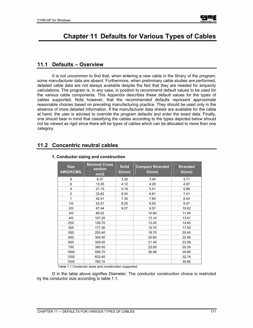
CYMCAP for Windows

CHAPTER 11 –- DEFAULTS FOR VARIOUS TYPES OF CABLES 171

Chapter 11 Defaults for Various Types of Cables

11.1 Defaults – Overview

It is not uncommon to find that, when entering a new cable in the library of the program, some manufacturer data are absent. Furthermore, when preliminary cable studies are performed, detailed cable data are not always available despite the fact that they are needed for ampacity calculations. The program is, in any case, in position to recommend default values to be used for the various cable components. This Appendix describes these default values for the types of cables supported. Note however, that the recommended defaults represent approximate reasonable choices based on prevailing manufacturing practice. They should be used only in the absence of more detailed information. If the manufacturer data sheets are available for the cable at hand, the user is advised to override the program defaults and enter the exact data. Finally, one should bear in mind that classifying the cables according to the types depicted below should not be viewed as rigid since there will be types of cables which can be allocated to more than one category.

11.2 Concentric neutral cables

1. Conductor sizing and construction

Size AWG/KCMIL

Nominal Cross section

mm2

Solid D(mm)

Compact Stranded D(mm)

Stranded D(mm)

8 8.37 3.26 3.40 3.71 6 13.30 4.12 4.29 4.67 4 21.15 5.19 5.41 5.89 2 33.62 6.54 6.81 7.41 1 42.41 7.35 7.60 8.43

1/0 53.51 8.25 8.55 9.47 2/0 67.44 9.27 9.57 10.62 3/0 85.02 10.80 11.94 4/0 107.20 12.10 13.41 250 126.70 13.20 14.60 350 177.30 15.70 17.30 500 253.40 18.70 20.65 600 304.00 20.60 22.68 650 329.40 21.40 23.59 750 380.00 23.00 25.35

1000 506.70 26.90 29.69 1250 633.40 32.74 1500 760.10 35.86

Table 1.1 Conductor sizes and construction supported.

D in the table above signifies Diameter. The conductor construction choice is restricted by the conductor size according to table 1.1.

CYMCAP for Windows

172 CHAPTER 11 –- DEFAULTS FOR VARIOUS TYPES OF CABLES

2. Conductor screen thickness

Conductor size (mm2) < 107.2 107.2 - 253.4 >253.4

Screen thickness (mm) 0.4 0.5 0.6 Table 1.2 Conductor screen thickness according to conductor size.

3. Insulation thickness

Rated kV Conductor size

(mm2) Insulation thickness

(mm) 5 8.37 - 506.7 2.29 > 506.7 3.55

8 13.3 - 506.7 2.92 > 506.7 4.44

15 32.62 - 506.7 4.44 > 506.7 5.58

25 All sizes 6.60 28 All sizes 7.11 35 All sizes 8.76 46 All sizes 11.56

>46 All sizes 11.56 Table 1.3 Insulation Thickness as per size and rated kV.

4. Insulation screen thickness

In the following table D stands for Diameter D over insulation(mm) <25.4 25.4-38.0 38.1-50.8 >50.8

Screen thickness (mm) 1.28 1.6 1.95 2.15 Table 1.4 Insulation screen thickness as per inner diameter

5. Jacket Thickness

In the following table D stands for diameter. D over everything but jacket (mm) <17.8 17.8-38.0 38.0-63.5 >63.5

Jacket thickness(mm) 1.2 1.6 2.2 2.9 Table 1.5 Jacket thickness as per inner diameter.

6. Concentric neutral

In the following table D stands for Diameter Conductor size Concentric wire D Number of wires

8 AWG 2.05 mm 11 6 AWG 2.05 mm 11 4 AWG 2.05 mm 11 2 AWG 2.05 mm 11 1 AWG 2.05 mm 11

1/0 AWG 2.05 mm 11 2/0 AWG 2.05 mm 14 3/0 AWG 2.05 mm 14 4/0 AWG 2.05 mm 22

250 KCMIL 2.05 mm 22 350 KCMIL 2.05 mm 18

CYMCAP for Windows


Conductor size Concentric wire D Number of wires 500 KCMIL 2.05 mm 26 600 KCMIL 2.05 mm 26 650 KCMIL 2.05 mm 26 750 KCMIL 2.58 mm 24

1000 KCMIL 2.58 mm 32 1250 KCMIL 2.58 mm 33 1500 KCMIL 2.58 mm 32

Table 1.6 Concentric neutral assembly as per conductor size.

The length of lay of the concentric neutral wires is taken to be 8 times the diameter of the cable under the wire assembly.

11.3 Extruded dielectric cables

1. Conductor sizes and construction

Same as for CONCENTRIC NEUTRAL CABLES. See table 1.1

2. Conductor screen thickness

Conductor area (mm2) 126.67 26.67-253.35 53.35-506.7 506.7

Conductor screen thickness (mm) 381 508 635 762 Table 2.1 Conductor screen thickness as per conductor size.

3. Insulation Thickness

Rated Voltage in kV

Conductor size in mm2

Insulation thickness in mm

46 126.67 13 126.67-1013.4 13

69 < 253.35 16.5 253.35-1013.4 16.5

115 760.00 20.32 760.00-1520.0 20.32

138 < 760.00 21.6 760.00-1520.0 21.6

Table 2.2 Insulation thickness as per size and rated kV.

4. Insulation screen thickness.

In the following table D stands for diameter D over insulation (mm) < 25.4 25.4-38.1 38.1-50.8 >50.8

Insulation screen thickness (mm) 1.27 1.6 1.96 2.16 Table 2.3 Insulation screen thickness as per inner diameter.

5. Jacket thickness

The jacket thickness is universally taken to be 2.5 mm.

CYMCAP for Windows


11.4 Low pressure oil filled cables (Type 3)

1. Conductor sizes and Construction

Conductor Size AWG or KCMILS

Nominal Cross section (mm2)

Compact Round D (mm)

Hollow core Outer D

(mm) 1/0 50 8.53 - 2/0 70 9.55 - 3/0 85 10.74 - 4/0 110 12.06 20 250 130 13.21 21 300 150 14.48 22 350 180 15.65 23 400 200 16.74 24 450 230 17.78 25 500 250 18.69 28 550 280 19.68 28 600 300 20.25 30 650 330 21.46 28 700 350 22.27 29 750 380 23.06 32 800 400 23.08 33 900 460 25.40 34

1000 510 26.90 35 1250 630 - 36 1500 760 - 39 2000 1010 - 44 2500 1270 - 49 3000 1520 - 54 3500 1770 - 57 4000 2030 - 61

Table 3.1 Conductor sizes and construction types.


2. Internal diameter for hollow conductor construction.

The default is universally taken to be 12.7 mm. (0.5 inch)

3. Conductor screen

Same as for EXTRUDED DIELECTRIC CABLES.

CYMCAP for Windows


4. Insulation Thickness

Rated Voltage in kV


15 2.54 25 3.43 35 4.32 46 5.21 63 6.73 69 7.24

115 11.05 120 11.43 130 12.20 138 12.83 161 13.46 230 19.30 345 26.29 500 34.01

Table 3.2 Insulation thickness as per rated kV.

5. Insulation screen


6. Jacket thickness

The jacket thickness is universally taken to be 2.5 mm.

11.5 High pressure oil (gas) filled cables

1. Conductor sizes and construction

4 or 6 Segments Sizes AWG/KCMIL

Nominal Cross Section (mm2)

Round D(mm) Stranded Compact D (mm)

3/0 85 11.9 10.7 - 4/0 107 13.4 12. - 250 127 14.6 13.2 - 300 157 16.0 14.5 - 350 177 17.3 15.6 - 400 203 18.5 16.7 - 450 228 19.6 17.8 - 500 257 20.6 18.7 - 550 279 21.7 19.7 - 600 304 22.7 20.7 - 650 329 23.6 21.5 - 700 355 24.4 22.3 - 750 380 25.3 23.1 - 800 405 26.2 23.8 - 900 456 27.2 25.4 -

1000 507 29.3 26.9 29.3 1250 633 32.7 - 32.7 1500 760 35.9 - 35.9 1750 887 38.8 - 38.8 2000 1013 41.5 - 41.5

CYMCAP for Windows


4 or 6 Segments Sizes AWG/KCMIL

Nominal Cross Section (mm2)

Round D(mm) Stranded Compact D (mm)

2250 1140 43.9 - 43.9 2500 1267 46.3 - 46.3 2750 1393 48.6 - 48.6 3000 1520 50.7 - 50.7 3250 1647 52.8 - 52.8 3500 1773 54.8 - 54.8 3750 1990 56.7 - 56.7 4000 2027 58.6 - 58.6

Table 4.1 Conductor sizes and construction types.


2. Conductor screen


3. Insulation thickness.

Rated Voltage in kV


69 6.86 115 10.67 120 11.05 138 12.45 161 14.86 230 18.92 345 25.91 500 27.94

Table 4.2 Insulation thickness as per rated LV level.

4. Insulation screen

Same as for extruded dielectric cables.

5. Skid Wires

• Skid Wire diameter is taken universally to be 5.08 mm. (0.2 inch)

• Number of skid wires is taken to be 2.

• Length of lay of skid wires is taken to be 76.2 mm. (3 inches)

CYMCAP for Windows


11.6 Sheath related defaults

1. Sheath Thickness.

The sheath thickness defaults described below pertain to all types of cables supported. They are compiled according to the practice followed for Low Pressure Oil Filled Cables. The calculation reads as follows:

Step A The quantities D1 and D2 are, at first, calculated based on whether the cable is a single conductor or a three core cable:

For Single conductor cables: D1 = ( D + 2T + 16 + 200 ) + 60 D2 = 1.03 ( D + 2T + 16 + 200 )

For three conductor cables: D1 = ( 2.155 D + 4.31 T + 207 + 40 ) + 60 D2 = 1.03 ( 2.155 D + 4.31 T + 207 + 40 )

where: D is the conductor diameter expressed in mils, T is the insulation thickness expressed in mils Xmm correspond to Ymils = (Xmm / 25.4 ) * 1000.00

Step B Take D3 = MAX ( D1, D2 )

Step C For LEAD sheath: S = 73.00 + 0.0270 D3 (mils)

The value calculated cannot be less than 110 (mils).

For SMOOTH ALUMINUM Sheath: S = 13.00 + 0.0400 D3 (mils)

For CORRUGATED ALUMINUM Sheath S = 19.90 + 0.0165 D3 (mils)

The inner radius of the corrugated sheath assembly is taken to be the cable radius under the sheath. The outer radius of the corrugated sheath assembly is by default taken to be the inner radius plus twice the sheath thickness computed above. The user should further adjust these dimensions for the particular case at hand if necessary.

2. Sheath Reinforcement Reinforcing tape thickness = 0.127 mm (0.005 inch) Tape over Insulation shield = 0.125 mm (0.0049 inch) Reinforcing tape width/metallic binder = 25.4 mm (1 inch) Number of reinforcing tapes = 2 Length of lay of tapes = 29.21 mm (1.25 inch) IEC related tape inclination = 54 degrees. Oversheath thickness = 2.0 mm (0.0787 inch)

CYMCAP for Windows


11.7 Armour related defaults

The defaults depicted here will universally apply for all types of cables equipped with armour protection.

1. Armour Bedding

Bedding Thickness in mm Cable Diameter under armour bedding in mm Tape Armour Wire Armour

0 - 11.43 .76 1.14 11.43 - 19.05 1.14 1.14 19.05 - 25.40 1.14 1.65 25.40 - 63.50 1.65 2.03

> 63.50 1.65 2.41 Table F.1 Armour Bedding as per inner Cable Diameter.

2. Armour Serving

Cable diameter under Armour Serving in mm

Serving Thickness in mm

0.00 - 19.05 1.27 19.05 - 38.10 1.65 38.10 - 57.15 2.03 57.15 - 76.20 2.41

> 76.20 2.79 Table F.2 Armour Serving as per inner Cable Diameter

3. Armour Tapes

Cable diameter under Bedding in mm

Tape Thickness in mm

0.00 - 25.40 0.51 > 25.40 0.76

Table F.3 Armour Tape thickness as per inner Cable Diameter.

4. Armour Wires

Cable diameter under Bedding in mm

Armour Wire Diameter in mm

0.00 - 19.05 2.11 19.05 - 25.40 2.77 25.40 - 43.18 3.40 43.18 - 63.50 4.19

> 63.50 5.16 Table F.4 Armour Wire size as per inner diameter.

• The armour wires are assumed to be TOUCHING and the necessary number is calculated from the cable dimensions.

• The length of lay of armour wires will be taken to be 1.3 times the diameter of the cable under armour.

11.7.1 Three core cables

The defaults for Conductor sizes and construction, Conductor shield, Insulation thickness and Insulation shield are the ones adopted for EXTRUDED DIELECTRIC CABLES.

Sheath, and Armour assemblies follow the general sheath and armour defaults.

CYMCAP for Windows

INDEX 1

INDEX

Accuracy of CYMCAP and References.....64 Additional cable installation salient aspects

...............................................................83 Ambient temperature and soil resistivity....76 Ampacity as a function of Temperature...133 Ampacity as a function of Time ...............133 Analysis options.........................................74 Append a database to another database 166 Approximate Temperature Field..............145 Armour Bedding/Armour Serving ..............27 Armour/Reinforcing tape............................26 Assign Loads to Cables...........................138 Automatic Design of Backfills/Duct Banks

.............................................................149 Backup the contents of the Working

directory to another directory ...............166 Barring certain bonding options.................87 Bonding......................................................84 Cable components, materials and

construction............................................17 Cable data in studies ...................................9 Cable design data window elements.........13 Cable Installation Data ..............................82 Cable Installation types .............................83 Cable layers...............................................35 Cable Library ...............................................9 Cable Library - Introduction .........................9 Cable Library data and executions............89 Cable library pop-up menu ........................12 Cable library window .................................10 Cable library window commands...............11 Cable transposition....................................87 Cables touching.........................................87 Case description and illustrations............136 Change the color of the curves for the

transient reports ...................................142 Change the connection line between the

cable and its associated label..............113 Change the properties of a label .............113 Concentric neutral cables........................171 Concentric neutral wires............................25 Conductor construction..............................19 Conductor data ..........................................18 Conductor material ....................................19 Conductor shield data................................21 Contents of CYMCAP..................................4

Convergence and the Selection of Reference Circuit ................................ 106

Copy selected items to a given data base............................................................ 168

Create a Load Curve using existing shapes.............................................................. 52

Creating a new cable ................................ 29 Creating a new duct bank......................... 40 Creating a new shape............................... 45 Creating a study........................................ 72 Curves and Shapes .................................. 43 Curves libraries command buttons ........... 52 Custom materials and thermal capacitances

.............................................................. 36 Customizing the Isotherms ..................... 147 CYMCAP GUI ............................................. 5 CYMCAP libraries and utilities - Overview . 5 CYMCAP menu for opened executions.. 158 CYMCAP Utilities .................................... 165 CYMCAP Utilities - Introduction.............. 165 Defaults – Overview................................ 171 Defaults for Various Types of Cables ..... 171 Define a new execution using an existing

one as template................................... 101 Defining a new study and a new execution

.............................................................. 91 Defining standard and/or non-standard duct

banks..................................................... 95 Defining the cable installation data........... 98 Defining the general installation data and

setup...................................................... 97 Designate AC conductor resistance values

............................................................ 163 Designate the AC system frequency for the

session ................................................ 163 Designate the Unit System for the session

............................................................ 163 Designate the working directory for

CYMCAP............................................. 165 Dielectric loss factors for insulating materials

.............................................................. 22 Drying and Impregnation .......................... 20 Duct bank Library - Introduction ............... 39 Duct bank/duct materials and construction87 Ductbank library management.................. 39 Enter a group of cables using absolute

coordinates.......................................... 103

CYMCAP for Windows

2 INDEX

Enter a trefoil formation using relative coordinates ..........................................103

Execution speed bar and associated command buttons ..................................93

Expanding and collapsing the curves........50 Extruded dielectric cables........................173 Filter Editor ................................................37 Fraction of return current for single phase

cables.....................................................88 General data for the installation ................76 Generate the reports ...............................140 Geometrical configuration of the installation

...............................................................82 Getting Started.............................................1 High pressure oil (gas) filled cables ........175 Importing a duct bank from the Library......96 Informing CYMCAP that a transient analysis

is to be performed ................................135 Installation steps – From a CD ....................2 Installation steps – From a downloaded file 3 Installing CYMCAP for Windows .................2 Insulation data ...........................................22 Insulation screen .......................................23 Jacket, oversheath and pipe coating

material ..................................................28 Keep all labels positions permanently .....115 Label grid editor.......................................111 Library of studies and executions..............67 Load and Heat Source Libraries

Management ..........................................49 Load Curve from field-recorded data.........57 Load-Curves/Heat Source Curves and

Shape Libraries......................................43 Low pressure oil filled cables (Type 3) ....174 Methodology and computational standards

...............................................................61 Modify the solution option from the

CYMCAP menu....................................102 Moisture migration modeling .....................77 Multiple cables per phase..........................82 Non isothermal earth surface modeling.....76 Opening more than one executions

simultaneously .....................................124 Other Libraries - Introduction.....................43 Overview of CYMCAP .................................1 Overview of CYMCAP menu ...................157 Particular modeling....................................35 Pipe material and dimensions ...................88 Populating the CYMCAP libraries ...............7 Preliminary considerations ......................129 Rearranging the cables in the proper ducts

.............................................................100 References ................................................66 Reset all labels to their default positions .114 Restore from floppy disk to a directory on

the hard-disk ........................................167

Results Reporting ................................... 108 Select/move/align labels ......................... 111 Setting the steady state analysis solution

Option.................................................... 92 Setting up the protection key ...................... 3 Shape Library Management ..................... 44 Sheath....................................................... 24 Sheath Reinforcing Material ..................... 24 Shifting a shape ........................................ 47 Simulation control parameters................ 162 Skid wires.................................................. 25 SL-type cables .......................................... 36 Software and hardware requirements ........ 2 Solve for Ampacity Given Time and

Temperature........................................ 130 Solve for Temperature given Time and

Ampacity.............................................. 131 Solve for Time given Ampacity and

Temperature........................................ 132 Specific cable installation data ................. 83 Specific installation data ......................... 108 Specify a “fixed ampacity circuit” ............ 105 Specify a heat source included in the

installation ........................................... 107 Specify the data for the transient analysis

option................................................... 137 Specify the transient analysis option ...... 137 Steady state analysis................................ 75 Steady state thermal analysis................... 90 Steady State Thermal Analysis................. 61 Steady State Thermal Analysis - General 61 Steady-state results labels...................... 109 Steps to create a new cable ..................... 16 Studies and executions............................. 66 Studies with CYMCAP ................................ 8 Study case for dissimilar directly buried

cables .................................................. 101 Study library pop-up menu........................ 68 Submit the simulation ............................. 139 Submitting more than one executions

simultaneously .................................... 127 Surrounding medium of the installation .... 77 Tabular Reports .............................. 118, 121 Tag specific items from the Libraries...... 167 Temperature as a function of Time......... 134 Temperature Field - Introduction ............ 145 Temperature Field – Scopes and Limitations

............................................................ 146 The CYMCAP Menu ............................... 157 The Ductbank Library ............................... 39 The Edit menu - Execution ..................... 159 The File menu - Execution...................... 158 The Files menu ....................................... 157 The Options menu - Execution ............... 160 The Sensitivity Analysis Option of CYMCAP

............................................................ 153

CYMCAP for Windows

INDEX 3

The View menu - Execution.....................159 The Windows menu.................................158 Three core cables....................................178 Trace the transients results with the mouse

.............................................................142 Transient Analysis ...................................129 Transient Analysis - Example and

Illustrations...........................................136 Transient Analysis - General ...................129

Transient analysis – How to proceed ..... 135 Transient analysis options ...................... 130 Useful considerations ............................... 35 View/hide labels...................................... 110 Viewing the graphical ampacity reports by

mouse selection .................................. 116 Windows Settings ....................................... 3 Working with more than one executions

simultaneously .................................... 127

Date post:	30-Nov-2015
Category:	Documents
Upload:	manoj
View:	1,681 times
Download:	247 times

Cymcap Manual

Documents