24
*
| Date post: | 13-Mar-2018 |
| Category: |
Documents |
| Upload: | duongnguyet |
| View: | 213 times |
| Download: | 0 times |

Household Food Demand in Nigeria: an Application of
Multivariate Double-hurdle Model
D. Akerele∗, R. Ti�n, & C. S. Srinivasan
8th April 2013
Paper prepared for presentation at the 87th Annual Conference of theAgricultural Economics Society, University of Warwick, United Kingdom
8 - 10 April 2013
Copyright 2013 by [Akerele, Ti�n & Srinivasan]. All rights reserved.Readers may make verbatim copies of this document for non-commercialpurposes by any means, provided that this copyright notice appears on allsuch copies.
Corresponding author: D. Akerele (e-mial: [email protected])
1

Household Food Demand in Nigeria: an Application of
Multivariate Double-hurdle Model
Abstract
A Bayesian approach was used to analyse household demand for sta-ples in Nigeria within the framework of a multivariate double-hurdle modelto account for censoring emanating from non-participation decisions. Wedemonstrate how to impose identi�cation constraints in the probit equationsand introduce a straightforward way of mapping observed and latent sharesin the demand (share) equations to satisfy adding up restrictions. Demandsfor cereals, beans and tubers are own-price inelastic with values close to unityin the lowest income quintile. Cross-price elasticities indicate demand pat-terns characterised by a mix of gross substitutability and complementarityrelationships among staple food subgroups. Presence of children and adoles-cents in the household as well as rural-urban and zonal (regional) di�erencesexact signi�cant in�uence on demand for staple foods. Total expenditureelasticities on staple food subgroups decline with higher income levels in linewith Engel's law. Cereals and tubers are all necessary goods in the mid-dle and highest income quintiles. However, they are luxury goods in thelowest income quintile. Our �ndings suggest that economic growth coupledwith targeted interventions such as cash or food stamp transfer programmesare crucial for improved consumption of major staples and nutrition amonghouseholds.
Key words: Bayesian approach, food demand, double-hurdle model,staples, Nigeria
JEL Code: D12
2

1 Introduction
Despite substantial e�orts to increase food supply through domestic pro-duction and massive importations over the past years, the rates of foodinsecurity and malnutrition in Nigeria is still alarming. Recent studies havereported food insecurity prevalence between 60 and 79 per cent among house-holds (Arene and Anyaeji, 2010; Orewa and Iyangbe, 2010; Olayemi, 2012;Omuemu et al., 2012) with incidence of malnutrition and related disordersspanning from 26.67 to 84.30 per cent in di�erent parts of the country(Akinyele, 2009; Goon et al., 2011; Aliyu et al., 2012; Ubesie et al., 2012).
Previous e�orts to enhance food security achieved limited successes asmost of the interventions concentrated more on the supply side of the prob-lem with little detailed evaluation of the demand side. Soaring prices of foodcommodities, inadequate purchasing powers, and income inequalities havebeen identi�ed, among others, as critical demand side factors stimulatingfood insecurity and malnutrition among the majority of households in Nige-ria and other developing countries (Obayelu, 2010; Olagunju et al., 2012;FAO, 2012). The greater burdens of food insecurity and malnutrition are of-ten endured by poor households. Over 70 percent of Nigerian households arepoor and expend between 60 to 80 percent or more of their earnings on food(Fregene and Bolorunduro, 2009; Adejobi and Babatunde, 2010; Obayelu,2010). Available statistics (national average) indicate that staples accountfor about 55 percent of the food budget in Nigeria (NBS, 2012) with mostpoor households devoting more than 60 percent of their food spending tostaples (Ashagidigbi et al., 2012; Ogunniyi et al., 2012).
The focus of this paper is on household demand for staples. Staplesare the main dietary sources of calories and proteins among Nigerian house-holds. They also constitute important sources of micro-nutrients in the dietsof many households (Gegios et al., 2010; Musa et al., 2012). The forego-ing underscores why detailed analysis of the structure of household demandfor staples is vital for food security and nutrition interventions in the coun-try, especially if policies are to impact on households through the market-place. And, in a highly strati�ed socioeconomic setting such as Nigeria,household food consumption responses to such interventions could vary byincome classes. Consequently, the �rst objective of this study is to examinehousehold demand for staples in Nigeria by income classes. We employ thehousehold data from the Nigeria Living Standard Survey (2003/2004) foranalysis.
One of the prominent attributes of cross-sectional (household) consump-tion studies is the preponderance of zero expenditure records (censoring in
3

the response/dependent variables); and how to appropriately handle themhas always been a major challenge confronting applied econometricians. Anumber of econometric models have been employed to handle the observedzeros with each model underpinned by di�erent hypotheses. These includethe Tobit model proposed by Tobin (1958) in which the observed zero ex-penditures are attributed purely to economic constraints. The model wasextended to a system of equations by Amemiya (1974) and have since beenapplied to several consumption studies (Perali and Chavas, 2000; Dong et al.,2004; Kasteridis and Yen, 2012). Following several criticisms of the tra-ditional Tobit model, Cragg (1971) introduced a two-step (double-hurdle)model which takes into account the fact that the observed zeros might alsobe linked to non-participation (abstention) decisions other than pure eco-nomic reasons. The model has also been employed in its variants (Yenand Jensen, 1996; Newman et al., 2001; Obayelu, Okoruwa and Oni, 2009;Akinbode and Dipeolu, 2012). The purchase infrequency model is anothereconometric model developed to account for the fact that the zero-valued ex-penditures might arise as a result of truncated sampling period as consumersmight be consuming from stock during the survey period or would have re-ported positive expenditures if the survey had spanned a longer period. Themodel has also been applied by several workers (Kimhi, 1999; Newman et al.,2001; Ti�n and Arnoult, 2010) on consumption studies. The p-tobit model(Deaton and Irish, 1984) and the double-hurdle model referred to as thepi-tobit model (Maki and Nishiyama, 1996; Maki and Garner, 2004) havealso been introduced to handle zero observations associated with genuinenon-consumption, purchase infrequency and misreporting.
In most cases, survey data do not provide detailed information regard-ing the sources of the observed zeros. In such situations, researchers areoften �compelled� to adopt a particular model on the basis of the assump-tions made about the potential sources of the zero observations (Kimhi,1999; Blisard and Blaylock, 1993)1 In this study, we attribute the observedzeros (censoring issues) in the household food consumption data to non-participation decisions. Hence, we employ the double-hurdle model for dataanalysis. The second objective of the study is to contribute to the literatureon censoring issues within demand systems by employing Bayesian approachto the estimation of multivariate double-hurdle (sample selection) model.
The remainder of the paper is scheduled as follows. We present thedouble-hurdle model in a multivariate framework in section 2 while estima-
1Some researchers also rely on the outcomes of statistical tests performed on a rangeof models deemed consistent with the data (Angulo et al., 2001; Newman et al., 2001).
4
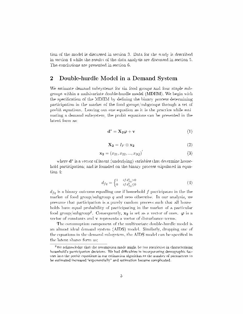
tion of the model is discussed in section 3. Data for the study is describedin section 4 while the results of the data analysis are discussed in section 5.The conclusions are presented in section 6.
2 Double-hurdle Model in a Demand System
We estimate demand subsystems for six food groups and four staple sub-groups within a multivariate double-hurdle model (MDHM). We begin withthe speci�cation of the MDHM by de�ning the binary process determiningparticipation in the market of the food groups/subgroups through a set ofprobit equations. Leaving out one equation as it is the practice while esti-mating a demand subsystem, the probit equations can be presented in thelatent form as:
d∗ = X2ϕ+ v (1)
X2 = IF ⊗ x2 (2)
x2 = (x21, x22, ..., x2Q)′
(3)
where d∗ is a vector of latent (underlying) variables that determine house-hold participation; and is founded on the binary process stipulated in equa-tion 4:
dfq ={1 if d∗fq>0
0 if d∗fq≤0(4)
dfq is a binary outcome equalling one if household f participates in the themarket of food group/subgroup q and zero otherwise. In our analysis, wepresume that participation is a purely random process such that all house-holds have equal probability of participating in the market of a particularfood group/subgroup2. Consequently, x2 is set as a vector of ones. ϕ is avector of constants and v represents a vector of disturbance terms.
The consumption component of the multivariate double-hurdle model isan almost ideal demand system (AIDS) model. Similarly, dropping one ofthe equations in the demand subsystem, the AIDS model can be speci�ed inthe latent shares form as:
2We acknowledge that the assumption made might be too restrictive in characterisinghousehold's participation decisions. We had di�culties in incorporating demographic fac-tors into the probit equations in our estimation algorithm as the number of parameters tobe estimated increased �exponentially� and estimation became complicated.
5

w∗ = X1Υ + u (5)
X1 = IF ⊗ x1 (6)
x1 = (x12, x12, ..., x1Q)′
(7)
x1q =
(1, lnp1,q, ..., lnpf+1,q, ln
(Eq
Pq
), S′q
)′, (8)
w∗ =(w∗1,1, w
∗1,2 ..., w
∗1,Q, , w
∗f,1, w
∗f,2 ..., w
∗f,Q,
)′, (9)
Υ =(α1, ψ1,1, ψ1,2, ..., ψ1,m+1, ω1, ς
′1, αf , ψf,1, ψf,2, ..., ψf,m+1, ωf , ς
′f
)′,
(10)
u = (u1,1, u1,1, ..., u1,Q, uf,1, uf,2, ..., uf,Q)′
(11)
Denoted by pfq is the price (index) of food group/subgroup f associatedwith household q, Eq is the total expenditure in the demand subsystem. De-noted by Pq =
∏f p
wfq
fq is the Stone's price index while Sq represents a vectorof demographic and other community/regional characteristics pertaining tohousehold q. Υ is a vector of coe�cients, u is a vector of disturbance termswhile w∗ is a vector of latent shares of food groups/subgroups in the demandsubsystem.
Drawing from Cragg (1971), the binary process stipulated in equation 4provides a linkage between the observed and the latent consumption (shares)of a multivariate double-hurdle model as follows:
wfq = w∗fq if dfq = 1 andw∗fq > 0 (12)
wfq = 0 if dfq = 0 andw∗fq > 0 (13)
or if dfq = 1 andw∗fq ≤ 0 (14)
or if dfq = 0 andw∗fq ≤ 0 (15)
6

where wfq is the observed share on food group/subgroup j by householdq. w∗fq is the associated latent share. In our studies, we assume that house-holds consume the groups/subgroups of food commodities being examinedat one time or the other. So, equations 14 and 15 are not considered.
Where positive consumption is recorded (in equation 12), it is possibleto formularise the mapping structure as:
wfq =w∗fq∑
f∈C w∗fq∀f ∈ C (16)
One key feature of equation 16 is that the latent shares of (positiveconsumption) adds up to unity. However, when the latent share(s) associ-ated with zero regime(s) (see equation 13) is/are added to the latent sharesof positive observation(s), the adding up property of demand is violated.The adding up (coherency) problem is resolved following Ti�n and Arnoult(2010) such that:
w∗fq = wfq
1−∑f /∈C
w∗fq
∀f ∈ C (17)
where w∗fq is the re-speci�ed latent shares which satis�es the adding uprestriction and
∑f /∈C w∗fq denotes the sum of the latent share(s) associated
with the observed zeros.The following conditions are imposed on the share equations in order to
conform with the properties of demand model. These include:homogeneity conditions which requires that∑
k
ψfg = 0 for all g, (18)
symmetry conditions which requires that
ψfg = ψgf for all f, g (19)
and concavity which requires that the Slutsky matrix (S) with elements:
Sfg = ψfg + ωfωgln
(E
P
)− wfδfg + wfwg (20)
is negative semi-de�nite. Where
δfg = 1 for f = g and δfg = 0 for f 6= g (21)
7

We follow Ti�n and Arnoult (2010) to impose homogeneity and symmetryrestrictions as
RΥ∗ = 0 (22)
where R is an r x F (F+2) matrix specifying the restrictions and Υ∗ denotesthe constrained version of matrix Υ. Incorporating the restrictions in ourmodel requires a re-parametrisation of the model. First, by specifying a(kF-r) x kF orthonormal matrix as:
RR′⊥ = 0 (23)
R⊥R′⊥ = I (24)
The restricted version of (Υ) can be stated as:
Υ∗ = R′⊥Υ (25)
where Υ is a (kF − r) x 1 vector of distinct parameters. Substitution ofequation 25 into equation 5 results into its restricted version speci�ed as:
w∗ = X1R′⊥Υ + u (26)
w∗ = AΥ + u (27)
whereA = X1R
′⊥ (28)
The AIDS model is estimated based on equation 27 but the restricted pa-rameters are regained from equation 25.
3 Bayesian Estimation
Prior to estimation, the sets of probit and demand equations are treated inthe form of seemingly unrelated regressions (SUR) as follows:
y∗ = Xβ + e, (29)
where
y∗ =(w∗′
, d∗′)′, X =
(A 00 X2
), β =
(Υ
′,ϕ
′)′, (30)
Presuming a di�use prior (Zellner, 1971:242) as:
8

p(β, Σ−1
)= p (β) p
(Σ−1
)∝ |Σ−1|
−(F+1)2 (31)
the conditional posterior distributions for β and Σ can be stated as:
p (β|y,X,Σ) ∼MVN
((Σ−1 ⊗X ′
X)−1 (
Σ−1 ⊗X ′)y∗,
(Σ−1 ⊗X ′
X))
(32)
p (Σ|y,X,β) ∼ IW(e′e, Q
)(33)
e =
u1,1 . . . uF,1 v1,1 . . . vF,1. .. .. .
u1,Q . . . uF,Q v1,Q . . . vF,Q
(34)
As earlier stated, the Slutsky matrix should be negative semi-de�niteto achieve concavity condition (see equation 20). Negativity condition isachieved, in practice, by specifying an accept/reject step in the estimationalgorithm such that only the draws (β ) from the distribution in equation32 which ful�ll the negativity condition are kept in the sample employed forinference.
It is important to note that the dependent variable (y∗) in equation 29contains both latent and observed elements. All the elements of the vector ofcontinuous (dependent) variables d∗ determining the binary outcomes andpart of the elements of w∗ associated with zero expenditures are latent (un-observed). Latency in both instances are regarded as missing data in thisstudy. We employ data augmentation strategy introduced by Tanner andWong (1987) to handle the missing (incomplete) data problems. Augment-ing observed (incomplete) data with latent data ensures unbiased estimation(Tanner and Wong, 1987). (Albert and Chib, 1993) demonstrate how toachieve data augmentation using the Gibbs sampler. They show that latentdata can be treated as additional blocks of unknown parameters in the es-timation algorithm if the conditional distributions of the latent data can beachieved. In our application, the Gibbs sampler was used to make iterativedraws from the conditional distributions of the latent data.
We now turn to the derivation of the conditional distributions. First, weconsider the conditional posterior for the missing data. Given the assump-tion that observations for a particular household are independent of the other
9

households, we introduce the conditional distributions by de�ning y∗q and y∗qto include exclusively the elements of y∗ and y∗ = Xβ which correspondto the respective qth household and draw the latent data on household ba-sis. Drawing latent data on food group/subgroup basis is also less di�cult.Hence, specifying the precision matrix ω = Σ−1, The conditional mean (Zfq)for each of the elements of y∗ can be speci�ed as:
Zfq = ˆy∗fq + ΣfΣ−1−f (y∗−f,q−y∗−f,q) = ˆy∗fq − ω−1ff ω−f (y∗−f,q−y∗−f,q) (35)
= ˆy∗fq − ω−1ff
∑f 6=g
ωgf (y∗−f,q−y∗−f,q) (36)
and the associated variance (ϑf ) expressed as:
ϑf = Σff −ΣfΣ−1−fΣ′−f = ω−1−f (37)
where ω = Σ−1 is the precision matrix, Σff is the fth on-diagonal elementof matrix (Σ), Σf is the fth row of Σ other than Σff , and Σ−f denotes thematrix within Σ after omitting both the fth column and fth row. ωff andω−f are speci�ed in the same way as Σff and Σ−f . yfq represents the �tted
value of yfq corresponding to the qth household. d−f,q and d−f,q are vectors
within d∗q and d∗q respectively, with their fth elements omitted. FollowingTi�n and Arnoult (2010), the missing data in the probit equations haveconditional distributions of the form:
dfq = 0 for d∗fq|d∗−f,q, β,X,Σ ∼N(Zfq, ϑf )I[−∞, 0] ∀f, q (38)
dfq = 1 for d∗fq|d∗−f,q, β,X,Σ ∼N(Zfq, ϑf )I[0,∞] ∀f, q (39)
and in the demand (share) equations, the form is:
wfq = 0 for w∗fq|d∗−f,q,Θ,X,Σ ∼N(Zfq, ϑf )I[0, 1] ∀f /∈C, q (40)
where I[−∞, 0] is an indicator variable equalling one if d∗fq ∈ [−∞, 0] and zero
otherwise. I[0,∞] and I[0, 1] are similarly speci�ed for d∗fq and w∗fq on theircorresponding intervals.
The next issue for discussion pertains to the identi�cation of the pro-bit equations. This is accomplished by putting restriction on the variance-covariance matrix:
10
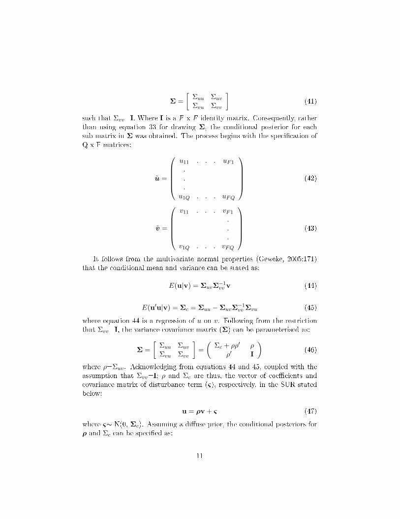
Σ =
[Σuu Σuv
Σvu Σvv
](41)
such that Σvv=I. Where I is a F x F identity matrix. Consequently, ratherthan using equation 33 for drawing Σ, the conditional posterior for eachsub-matrix in Σ was obtained. The process begins with the speci�cation ofQ x F matrices:
u =
u11 . . . uF1
.
.
.u1Q . . . uFQ
(42)
v =
v11 . . . vF1
.
.
.v1Q . . . vFQ
(43)
It follows from the multivariate normal properties (Geweke, 2005:171)that the conditional mean and variance can be stated as:
E(u|v) = ΣuvΣ−1vv v (44)
E(u′u|v) = Σc = Σuu −ΣuvΣ−1vv Σvu (45)
where equation 44 is a regression of u on v. Following from the restrictionthat Σvv=I, the variance-covariance matrix (Σ) can be parameterised as:
Σ =
[Σuu Σuv
Σvu Σvv
]=
(Σc + ρρ′ ρ
ρ′ I
)(46)
where ρ=Σuv. Acknowledging from equations 44 and 45, coupled with theassumption that Σvv=I; ρ and Σc are thus, the vector of coe�cients andcovariance matrix of disturbance term (ς), respectively, in the SUR statedbelow:
u = ρv + ς (47)
where ς∼ N(0, Σc). Assuming a di�use prior, the conditional posteriors forρ and Σc can be speci�ed as:
11

ρ|Σ−1c ∼ N[(
uΣ−1c u)−1
u′v,(uΣ−1c u
)−1](48)
and
Σ−1c |% ∼ IW (ς ′ς, Q) (49)
respectively. ρ and Σc are employed in the relations indicated in equation46 as the groundwork for sampling the restricted variance-covariance matrix(equation 46). The estimation algorithm is stipulated in subsection 3.1.
3.1 Estimation (Gibbs) Algorithm
The estimation algorithm describes the key steps involved in estimating theparameters of the model. The estimation algorithm are systematically pre-sented below.
1. Assume (select) the starting values for y∗ and Σ.2. Employ the newly drawn values of y∗ obtained from Steps 4 and 5
and Σ generated from Step 6 or those presumed in Step 1 (in case this isthe �rst draw) to draw the vector of parameters (β).
3. Calculate the Slutsky matrix from equation 20 using the appropriateelements of β and check if the matrix is negative semi-de�nite. If so, includethe drawn (sampled) vector of parameters (β). Otherwise, go back to theformer (immediate past) draw of β.
4. With the vectors of parameters (β) generated in Step 2, computey∗ = Xβ. Employ the appropriate elements in y∗ and Σ from step 6 or theassumed starting values in Step 1 (in case this is the �rst draw) to estimatethe mean as well as the variance of conditional distributions from equations36 and 37.
5 (a) To obtain the latent (missing) data for the probit equations, applythe appropriate mean and variance obtained from Step 4 to draw from thetruncated normal distributions speci�ed in equations 38 and 39.
5 (b) To generate latent data for the demand (share) equations wherezero expenditures are reported, utilise the appropriate mean and varianceobtained from Step 4 to take draws from the truncated normal distributionsin equations 40.
6. Use β obtained from Step 2 and y∗ from Steps 4 and 5 to drawcovariance matrix Σ.
7. Draw ρ from the normal distribution in equation 488. Draw Σc from the inverted Wishart distribution in equation 49.9. Use ρ and Σc to complete the covariance matrix Σ in equation 46.
12

10. Return to Step 2.
4 Description of Data
The Nigeria Living Standard Survey (NLSS) 2003/2004 household data andthe food price data for 2003/2004 obtained from the National Bureau ofStatistics, Nigeria are employed for this study. The NLSS data is the largest,most comprehensive available micro-data in the country which can be usedfor demand analysis. The NLSS data were collected at the household levelsfrom rural and urban sectors in various enumeration areas across the 36states of the country including the federal capital territory (Abuja) througha two-stage strati�ed sampling technique from September, 2003 to August2004. A total of 19158 households were sampled by means of questionnaire.The price data were collected on a monthly for the year 2003 and 2004 inboth rural and urban sectors across the 36 states of the country includingAbuja and in most of the enumeration areas covered by the household survey(NLSS). The food items in the food price �le correspond with those in theNLSS data. There are 70 food items in the price �le excluding tobacco.
The NLSS household data were compiled in di�erent �les having namesthat suitably describe the items contained in them. Although data collectedcovers di�erent aspects of household livelihoods, data on food purchased inthe markets (from food purchase �le), quantities of food consumed out ofwhat the household produce (from own-consumption �le) and data from thethe household expenditures and socio-demographic characteristics �les arerelevant to the study. Food data were collected from each household on aweekly basis over a period of six consecutive weeks. The values of foodspurchased in the markets were recorded in the Naria (national currency)while the quantities of foods consumed from household production were re-ported either in the standard or local measures. There are e�ectively 133food items listed in the food �les besides tobacco and cigarettes. However,not all household reported consumption of the entire food items. The own-consumption �le also contains information on the amount (price) each of the�own-consumed� food items could be sold for in the market. These prices arereferred to as proxy prices in this study. The food quantities were convertedto kilogramme and the associated prices expressed in price/kilogramme.
Relevant data in the household expenditure and demographic characteris-tics �le include expenditure on non-food items and non-food price index; age,gender and educational status of household head; the sector (rural/urban)and the geopolitical zone where household belongs; Food and Agriculture
13

Organization (FAO) adult equivalent (AE) household size and dates of �rstvisit to each household. Each of the NLSS household data �les contains in-formation on the states, sectors, enumeration areas and household numbers(unique identi�ers). The NLSS household data �les were �rst merged to-gether based on these information. There are 18880 households that mergedfrom all the household data �les. The resultant bigger �le is referred to ashousehold data �le.
Thereafter, the food price data were merged with the already mergedhousehold data �led based on state, sectors, enumeration areas and monthand year of data collection. Households in a given enumeration area are pre-sumed to be facing similar market price situation. Only 13950 householdsof entire households eventually merged successfully with the food price dataas some enumeration areas and months in the price �le do not merge per-fectly with the those in the NLSS household data �le. Where a food itemis consumed and the price is not available in the food price �le, the averageof the proxy price reported of the particular food items reported by house-hold(s) in the corresponding enumeration area, sector or state is computedand applied as the market price. Estimated expenditures on own-consumedfoods were computed and added to the corresponding food expenditure datafrom the food purchase �le. Expenditures on food and non food items wereconverted to monthly information and discounted by the adult equivalenthousehold size. The per capita adult equivalent information are used foranalysis. Households with per capita calorie intake below 500 kcal per daywere removed from the 13950 households as hardly would an average adultsurvive with that daily intake level. A total of 13142 households were �nallyemployed for analysis.
For the purpose of analysis, we �rst partition items into two categories-food and non-food items. The entire food entire were also divided into sixgroups (staples, animal products, beverages, fruits vegetables, fats and oilsand seeds and nuts). Since our focus is on staple, we limit further parti-tioning to staples. We classi�ed staples into four food subgroups namely:cereals, beans, tubers and snacks. Classi�cation of foods items are basedon previous studies on food demand and nutrition in the country (Oguntonaand Akinyele, 1995; Maziya-Dixon et al., 2004; Obayelu, Okoruwa and Ajani,2009). The proportion of households having zero consumption records on ce-reals, beans, tubers and snacks is approximately 1.33, 24, 20.33 and 77.66per cent respectively. We constructed the Thornqvist Theil price index torepresent the price of each food aggregates.
We estimated demand models at hierarchy of three budgeting stages. Atthe �rst stage, we estimated a single demand (share) equation with aggregate
14

food budget share as dependent variable. The second stage featured estima-tion of demand subsystem for the six food groups while the third stage in-volved estimation of a demand subsystem for the four staple food subgroups.We employ the appropriate elasticities obtained from the estimated demandmodels to compute unconditional price and total expenditure elasticities forthe four staple food subgroups following Edgerton (1997). Households weregrouped into �ve income quintiles in order to explore di�erences in house-hold demand responses.The demographic variables included in the demandequations are presented in Table 1.
15
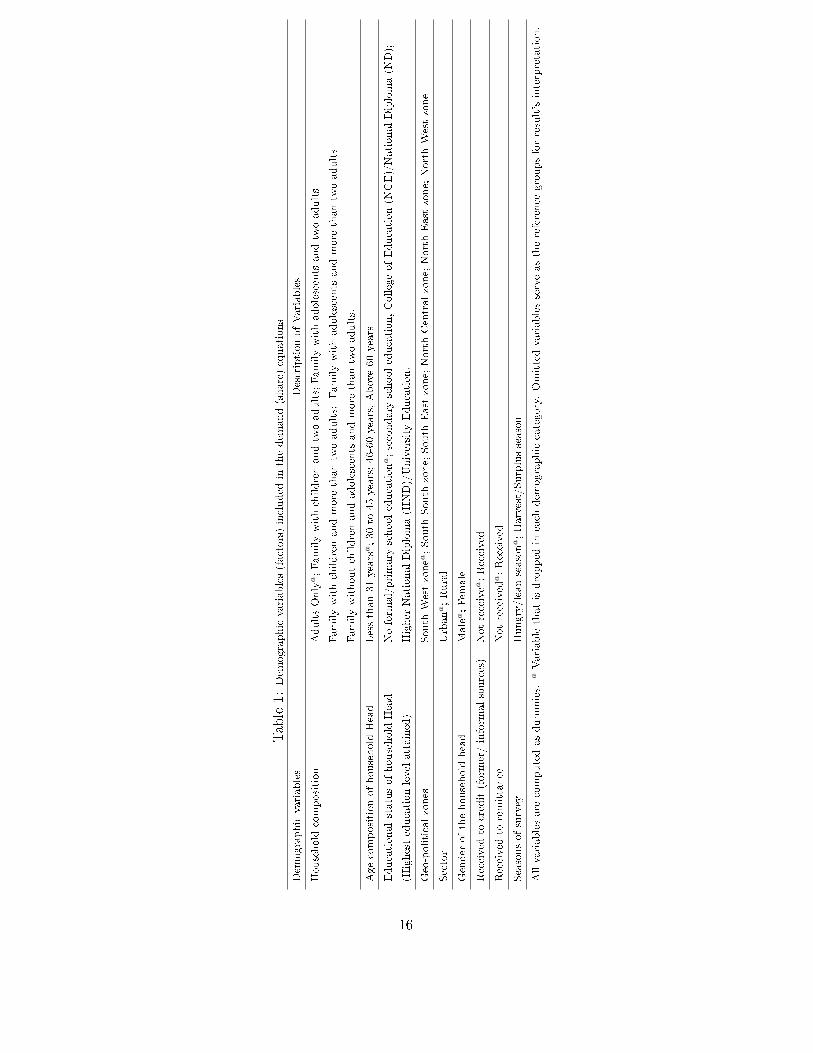
Table1:
Dem
ographicvariables(factors)included
inthedem
and(share)equations
Dem
ographicvariables
DescriptionofVariables
Household
composition
AdultsOnly
a;Familywithchildrenandtwoadults;Familywithadolescents
andtwoadults
Familywithchildrenandmore
thantwoadults;
Familywithadolescents
andmore
thantwoadults
Familywithoutchildrenandadolescents
andmore
thantwoadults.
Agecompositionofhousehold
Head
Lessthan31years
a;30to
45years;46-60years,Above60years
Educationalstatusofhousehold
Head
Noform
al/primary
schooleducationa;secondary
schooleducation,CollegeofEducation(N
CE)/NationalDiploma(N
D);
(Highesteducationlevelattained)
Higher
NationalDiploma(H
ND)/University
Education.
Geo-politicalzones
South
Westzonea;South
South
zone;South
East
zone;NorthCentralzone;NorthEast
zone;NorthWestzone
Sector
Urbana;Rural
Gender
ofthehousehold
head
Male
a;Fem
ale
Received
tocredit(form
er/inform
alsources)
Notreceivea;Received
Received
toremittance
Notreceived
a;Received
Seasonsofsurvey
Hungry/leanseasona;Harvest/Surplusseason
Allvariablesare
computedasdummies.
aVariablethatisdropped
ineach
dem
ographiccategory.Omittedvariablesserveasthereference
groupsforresult'sinterpretation.
16

5 Results and Discussion
The results of the unconditional price and total expenditure elasticities forcereals, beans, tubers and snacks are presented in Table 2. We do not reportthe results of the compensated and uncompensated elasticities obtained ateach stage of the hierarchy in this paper. They are available on request.However, we present the results of demographic factors in�uencing demandfor staple food subgroups (Table 3). All the parameters reported are themean values generated from the Gibbs sample. For brevity, we present resultsfor the lowest, middle (third) and the highest income quintiles.
Table 2 shows that all own price elasticities have the expected negativesigns. This is a result of the negativity constraint imposed on the curvatureof the expenditure function. Snacks has the largest own-price elasticitiesin each of the income quintiles; suggesting that demand for snacks is themost sensitive to changes in own-price. Own-price elasticities of cereals areconsistently high in the lowest, middle and highest income quintiles withvalues -0.938, -0.926 and -1.018 respectively. This indicates that householdsin the highest income quintile are the most sensitive to changes in cerealprices. Although demand for cereals is own-price inelastic in the lowest andthe middle income quintiles, elasticity values are close to unity. Demand forcereals is own-price elastic in the highest income quintile.
Cross-price elasticities indicate a mix of gross substitutability and com-plementarity relationships among staple food subgroups; indicating the roleof total expenditure (income) e�ects in stimulating cross-price responsivenessto food consumption among households. The complementary relationshipsfound between tubers and beans in the lowest and middle income quintiles areexpected. Households in Nigeria consume tubers such as yam and cocoyamwith beans in form of porridge. Consumption of tubers and tuber productswith bean cakes/meals and bean soups are also common, especially in thesouthern parts of the country. Total expenditure (income) elasticities on foodsubgroups decline with higher income levels in line with the Engel's, law. Allstaple food subgroups are normal goods across income quintiles except forsnack food subgroup which appears as inferior good in the highest incomequintile. Cereals and tubers have the highest total expenditure elasticitiesand are luxury goods among households in the lowest income quintile. Thissuggests that an average household in the poorest segment of the populationwill increase consumption of tubers and cereals more than other staple foodsif household income improves.
We now consider the in�uence of demographic factors on demand forstaple food subgroups (Table 3). We indicate a signi�cant variable with an
17

asterisk; showing that the 95 percentiles of its highest HPDIs excludes zero.The results of snacks subgroup are excluded as none of the demographicvariables included in the model had signi�cant e�ects on its demand. Theresults indicate that rural households in the middle and the highest incomequintiles consume more tubers and less beans than there urban counterparts.Variations in demand for staple food subgroups at the zonal levels is alsowell pronounced. For instance, while consumption of cereals is higher in theNorth Central, North East and North West zones, consumption is lower inthe South South and South East zones. The opposite is the case for tubers.Presence of children and adolescents in the households leads to high demandfor tubers. Demand for tubers is also higher among household headed byolder people compared to households headed by people below 31 years.
6 Conclusions
A major challenge confronting applied econometricians is how to suitablymodel the zero-valued observations (censoring) in the dependent variableswhile estimating demand systems using microdata. In this paper, we ap-plied a Bayesian approach to estimate household food demand systems usinga multivariate double-hurdle model to handle zero observations attributableto non-participation decisions. Demand patterns feature a mix of gross sub-stitutability and complementarity among staple food subgroups, indicatingthe importance of total expenditure(income) e�ect in determining cross-priceresponsiveness. Presence of children and adolescents, rural-urban and zonal(regional) variations and age of household head, among others, have signif-icant in�uence on demand for cereals, beans and tubers. Total expenditure(income) elasticities on food subgroups decline with higher income levels.
Although cereals, beans and tubers are normal goods, they are all nec-essary goods in the middle and highest income quintiles. Total expenditureelasticities of cereals and tubers greater than unity in the lowest incomequintile. The implication is that improved income would lead to higher con-sumption of cereals and tubers among households in the poorest incomequintile. In sum, while income growth would enhance consumption of sta-ples among households generally, targeted interventions such as cash or foodstamp transfers are advocated to boost access to major staple foods amongthe poorest household groups in the country.
18

Table 2: Unconditional elasticities for staple food subgroups
Quantity Price Total expenditure
Cereals Beans Tubers Snacks elasticity
Lowest income quintile
Cereals -0.938 0.018 0.041 -0.054 1.039
Beans 0.419 -0.968 -0.093 0.115 0.586
Tubers 0.060 -0.080 -0.915 -0.029 1.073
Snacks 1.623 1.765 1.477 -5.475 0.677
Middle income quintile
Cereals -0.926 0.076 0.041 0.072 0.806
Beans 0.502 -0.847 0.034 -0.145 0.498
Tubers -0.008 -0.024 -0.799 -0.010 0.919
Snacks 1.101 -0.290 0.197 -1.509 0.547
Highest income quintile
Cereals -1.018 0.083 0.257 0.079 0.184
Beans 0.365 -0.928 0.125 -0.047 0.149
Tubers 0.219 0.015 -0.835 -0.065 0.204
Snacks 7.544 -0.414 -2.667 -3.667 -0.245
19
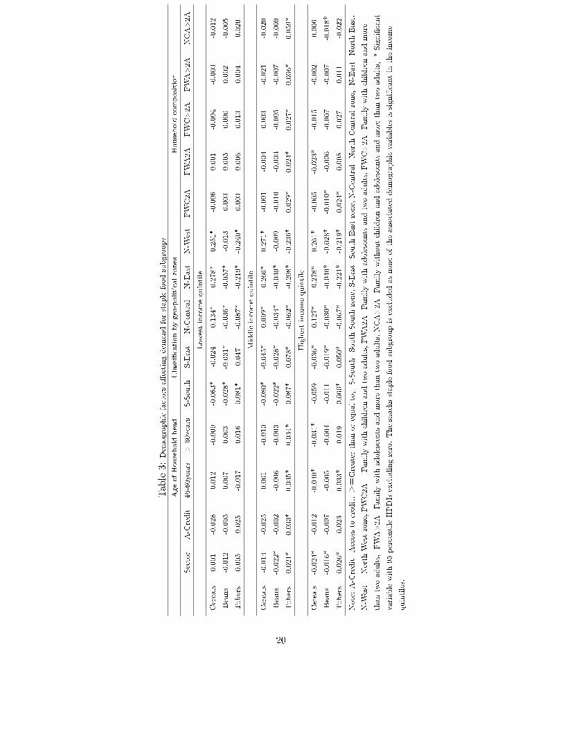
Table3:
Dem
ographicfactors
a�ectingdem
andforstaplefoodsubgroups
AgeofHousehold
head
Classi�cationbygeo-politicalzones
Household
composition
Sector
A-Credit
46-60years
>60years
S-South
S-East
N-Central
N-East
N-W
est
FWC2A
FWA2A
FWC>2A
FWA>2A
NCA>2A
Low
estincomequintile
Cereals
0.001
-0.028
0.012
-0.009
-0.063*
-0.024
0.134*
0.278*
0.251*
-0.006
0.001
-0.004
-0.003
-0.012
Beans
-0.012
-0.005
0.007
0.003
-0.028*
-0.031*
-0.036*
-0.057*
-0.013
0.003
0.005
0.000
0.002
-0.005
Tubers
0.005
0.025
-0.017
0.016
0.081*
0.047
-0.087*
-0.219*
-0.240*
0.003
0.006
0.013
0.004
0.020
Middleincomequintile
Cereals
-0.014
-0.025
0.001
-0.010
-0.080*
-0.045*
0.099*
0.260*
0.271*
-0.001
-0.004
0.003
-0.021
-0.020
Beans
-0.022*
-0.002
-0.006
-0.003
-0.022*
-0.028*
-0.034*
-0.039*
-0.009
-0.010
-0.003
-0.005
-0.007
-0.009
Tubers
0.021*
0.033*
0.035*
0.034*
0.087*
0.078*
-0.062*
-0.208*
-0.236*
0.029*
0.024*
0.027*
0.036*
0.059*
Highestincomequintile
Cereals
-0.024*
-0.012
-0.040*
-0.031*
-0.059
-0.036*
0.127*
0.278*
0.261*
-0.005
-0.023*
-0.015
-0.002
0.006
Beans
-0.016*
-0.007
-0.005
-0.004
-0.011
-0.019*
-0.030*
-0.040*
-0.028*
-0.010*
-0.006
-0.007
-0.007
-0.018*
Tubers
0.026*
0.023
0.033*
0.019
0.066*
0.050*
-0.067*
-0.221*
-0.219*
0.024*
0.008
0.027
0.011
-0.022
Note:A-Credit=Accessto
credit,>=Greaterthanorequalto,
S-South=South
South
zone,S-East=South
East
zone,N-Central=NorthCentralzone,
N-East=NorthEast,
N-W
est=
NorthWestzone,FWC2A=
Familywithchildrenandtwoadults,FWA2A=Familywithadolescents
andtwoadults,FWC>2A=Familywithchildrenandmore
thantwoadults,
FWA>2A=Familywithadolescents
andmore
thantwoadults,NCA>2A=Familywithoutchildrenandadolescents
andmore
thantwoadults,
*Signi�cant
variablewith95percentileHPDIsexcludingzero.Thesnacksstaplefoodsubgroupisexcluded
asnoneoftheassociateddem
ographicvariablesissigni�cantin
theincome
quintiles.
20
References
Adejobi, A. O. and Babatunde, R. O. (2010). Analysing the level of marketorientation among rural farming households in northern Nigeria, AfricanJournal of General Agriculture 6(4): 255�261.
Akinbode, S. O. and Dipeolu (2012). Double-hurdle model of fresh �sh con-sumption among urban households in South-West Nigeria, Current Re-search Journal of Social Sciences 4(6): 431�439.
Akinyele, I. O. (2009). Ensuring food and nutrition security in rural Ni-geria: an assessment of the challenges, information needs, and analyticalcapacity. Nigeria Strategy Support Program (NSSP) Background paper 7,International Food Policy and Research Institute.
Albert, J. A. and Chib, S. (1993). Bayesian analysis of binary and poly-chotomous response data, Journal of the American Statistical Association
88(422): 669�679.
Aliyu, A. A., Oguntunde, O. O., Dahiru, T. and Raji, T. (2012). Prevalenceand determinants of malnutrition among pre-school children in northernNigeria, Pakistan Journal of Nutrition 11(11): 1092�1095.
Amemiya, T. (1974). Multivariate regression and simultaneous equationmodels when the dependent variables are truncated normal, Econometrica42: 999�1012.
Angulo, A. M., Gil, J. M. and Gracia, A. (2001). The demand fror alcoholicbeverages in Spain, Agricultural Economics 26(2001): 71�83.
Arene, C. J. and Anyaeji, R. C. (2010). Determinants of food security amonghouseholds in nsukka metropolis of enugu state, nigeria, Pakistan Journal
of Social Sciences 30(1): 9�16.
Ashagidigbi, W. M., Yusuf, S. A. and Okoruwa, V. O. (2012). Determinantsof households' food demand in nigeria,World Rural Observations 4(4): 17�28.
Blisard, N. and Blaylock, J. (1993). Distinguishing between market parti-cipation and infrequency of purchase models of butter demand, AmericanJournal of Agricultural Economics 75: 314�320.
21

Cragg, J. G. (1971). Some statistical models for limited dependent variableswith application to the demand for durables, Econometrica 39(5): 829�844.
Deaton, A. and Irish, M. (1984). Statistical models for zero expenditures inhousehold budgets, Journal of Public Economics 23(1-2): 59�80.
Dong, D. D., Gould, B. W. and Kaiser, H. M. (2004). Food demand inmexico: An application of the ameniya-tobin approach to the estimationof a censored food system, American Journal of Agricultural Economics
86(4): 1094�1107.
Edgerton, D. L. (1997). Weak separability and the estimation of elasticity inmultistage demand system, American Journal of Agricultural Economics
79(1): 62�79.
FAO (2012). The state of food insecurity in the world 2012. Rome , (Availableat http://www.fao.org/docrep/016/i3027e/i3027e.pdf).
Fregene, T. B. and Bolorunduro, P. I. (2009). Role of women in food securityand seasonal variation of expenditure pattern in coastal �shing communit-ies in Lagos State, Journal of Agricultural Extension 13 (2): 21�33.
Gegios, A., Amthor, R., Maziya-Dixon, B., Egesi, C., Mallowa, S., Nungo,R., Gichuki, S., Mbanaso, A. and Manary, M. J. (2010). Children con-suming cassava as a staple food are at risk for inadequate zinc, iron, andvitamin a intake, Plant Foods for Human Nutrition 65(1): 64�70.
Geweke, J. (2005). Contemporary Bayesian Econometrics and Statistics,New Jersey, USA, Wiley & Son Inc.
Goon, D. T., Toriola, A. L., Shaw, B. S., Amusa, L. O., Monyeki, M. A.,Akinyemi, O. and Alabi, O. A. (2011). Anthropometrically determinednutritional status of urban primary schoolchildren in Makurdi, Nigeria,BMC Public Health 11:769: 1�8.
Kasteridis, P. and Yen, S. (2012). U.S. demand for organic and conventionalvegetables: a Bayesian censored system approach, Australian Journal of
Agricultural and Resource Economics 56(3): 405�425.
Kimhi, A. (1999). Double-hurdle and purchase-infrequency demand analysis:a feasible integrated approach, European Review of Agricultural Economics
26(4): 425�442.
22

Maki, A. and Garner, T. I. (2004). The gap between macro and micro eco-nomic statistics: Estimation of the misreporting model using micro-datasets, Available at http://repec.org/esAUSM04/up.17601.1075102278.pdf.
Maki, A. and Nishiyama, B. (1996). An analysis of under-reporting for micro-data sets: The misreporting or double-hurdle model, Economics Letters
52(3): 211�220.
Maziya-Dixon, B. M., Akinyele, I. O., Oguntona, E. B., Nokoe, S., Sanusi,R. A. and Harris, E. (2004). Nigeria food consumption and nutrition sur-
vey 2001-2003 Summary, International Institute of Tropical Agriculture(IITA).
Musa, U., Hati, S. S. and Mustapha, A. (2012). Levels of fe and zn in staplecereals: Micronutrient de�ciency implications in rural northeast Nigeria,Food and Public Health 2(2): 28�33.
NBS (2012). Consumption pattern in nigeria 2009/10: Preliminary report(2012), (Available at http://www.nigerianstat.gov.ng/).
Newman, C., Henchion, C. and Matthews, A. (2001). Infrequency of purchaseand double-hurdle models of irish households' meat expenditure, EuropeanReview of Agricultural Economics 28(4): 393�412.
Obayelu, A. E. (2010). Global food price increases and nutritional status ofNigerians: the determinants, coping strategies, policy responses and im-plications, ARPN Journal of Agricultural and Biological Science 5(2): 67�80.
Obayelu, A. E., Okoruwa, V. O. and Ajani, O. I. Y. (2009). Cross-sectionalanalysis of food demand in the north central, nigeria: The quadratic al-most ideal demand system (quaids) approach, China Agricultural Eco-
nomic Review 1(2): 173�193.
Obayelu, A. E., Okoruwa, V. O. and Oni, O. A. (2009). Analysis of ruraland urban households' food consumption di�erential in the north-central,nigeria: A micro-econometric approach, Journal of Development and Ag-
ricultural Economics 1(2): 18�26.
Ogunniyi, L. T., Ajao, A. O. and Oladejo, J. A. (2012). Food consump-tion patterns in ogbomoso metropolis of Oyo State, Nigeria, Journal ofAgriculture and Social Research 12(1): 74�83.
23

Oguntona, E. B. and Akinyele, I. O. (1995). Nutrient Composition of Com-
monly Eaten Food in Nigeria -Raw, Processed and Prepared, Food BasketFoundation, Ibadan.
Olagunju, F. I., Oke, J. T. O., Babatunde, R. and Ajiboye, A. (2012). De-terminants of food insecurity in ogbomoso metropolis of oyo state, nigeria,PAT 8 (1): 111�124.
Olayemi, A. O. (2012). E�ects of family size on household food security inOsun State, Nigeria, Asian Journal of Agriculture and Rural Development
2(2): 136�141.
Omuemu, V. O., Otasowie, E. M. and Onyiriuka, U. (2012). Prevalenceof food insecurity in Egor local government area of Edo State, Nigeria,Annals of African Medicine 11(3): 139�145.
Orewa, S. I. and Iyangbe, C. (2010). The struggle against hunger: thevictims and the food security strategies adopted in adverse conditions,World Journal of Agricultural Sciences 6(6): 740�745.
Perali, F. and Chavas, J. (2000). Estimation of censored demand equationsfrom large cross-section data, American Journal of Agricultural Economics
82(4): 1022�1037.
Tanner, M. A. and Wong, W. H. (1987). The calculation of posterior distri-butions by data augmentation, Journal of the American Statistical Asso-
ciation 82(398): 528�540.
Ti�n, R. and Arnoult, M. (2010). The demand for a healthy diet: estimatingthe almost ideal demand system with infrequency of purchase, EuropeanReview of Agricultural Economics 37(4): 501�521.
Tobin, J. (1958). Estimation of relationships for limited dependent variables,Econometrica 26: 24�36.
Ubesie, A. C., Ibeziako, N. S., Ndiokwelu, C. I., Uzoka, C. M. and Nwafor,C. A. (2012). Under-�ve protein energy malnutrition admitted at theUniversity of Nigeria Teaching Hospital, Enugu: a 10 year retrospectivereview, Nutrition Journal 11(43): 1�7.
Yen, S. T. and Jensen, H. H. (1996). Determinants of household expenditureson alcohol, Journal of Consumer A�airs, Summer 30(1): 48�67.
Zellner, A. (1971). An Introduction to Bayesian Inference in Econometrics.
24


