ISSN 1063-7788, Physics of Atomic Nuclei, 2013, Vol. 76, No. 10, pp. 1301–1307. c© Pleiades Publishing, Ltd., 2013.

ELEMENTARY PARTICLES AND FIELDSTheory

DDD-Dimensional Smorodinsky–Winternitz Potential:Coherent State Approach∗

Nuri Unal**

Akdeniz University, Department of Physics, Antalya, TurkeyReceived May 29, 2012

Abstract—In this study, we construct the coherent states for a particle in the D-dimensional maximallysuperintegrable Smorodinsky–Winternitz potential. We, first, map the system into 2D harmonic oscilla-tors, second, construct the coherent states of them by evaluating the transition amplitudes. Third, in theCartesian and the hyperspherical coordinates, we find the coherent states and the stationary states of theoriginal sytem by reduction.

DOI: 10.1134/S1063778813090202

1. INTRODUCTION

The most familiar examples of the maximally su-perintegrable systems are the Kepler–Coulomb prob-lem in 2 and 3 dimensions [1–3] and the harmonicoscillator [4, 5]. First, Smorodinsky, Winternitz,and their collaborators searched the generalizationsof the Kepler–Coulomb problem and the harmonicoscillators in 2-dimensional systems [6–8]. Max-imally superintegrable quantum systems appear inmany domains of physics. Later, Evans discussedthe generalization of the Smorodinsky–Winternitzpotentials in 3 dimensions [9]. In these studies, theintegrals of motion are first or second order withrespect to momenta. Kalnins, Kress, and Millerand Daskaloyannis and his collaborators obtained thecomplete classification of the second-order superin-tegrable systems [10–16].

Grosch and his collaborators discussed the so-lution of the quantum problem for two- and three-dimensional Smorodinsky–Winternitz potentials byusing the path integrals [17]. In a recent paper,Quesno discussed the solution of the quantum prob-lem for a particle in D-dimensional generalization ofthe Smorodinsky–Winternitz potentials [18].

First, Schrodinger derived the coherent states forthe one-dimensional harmonic oscillator [19]. Theseare eigenstates of the lowering operator of the har-monic oscillator with complex time-dependent eigen-values and satisfy the minimum uncertainty relationsand are used in the quantum theory of the electro-dynamics in 1963 and recognized as the Glauber

∗The text was submitted by the author in English.**E-mail: nuriunal@akdeniz.edu.tr

states [20]. Brown and, later, Nieto and Simmons de-veloped a general formalism to construct the coherentstates for the different potentials with some dynamicalsymmetry groups [21, 22].

In usual formulation, the Feynman path integralsgive the transition amplitudes between the configu-ration space eigenstates of the particle. In 1998, wederived the transition amplitudes between the eigen-states of the lowering operator for a particle in theharmonic oscillator, and defined the coherent statesin terms of these amplitudes by using a complemen-tary formulation of the Feynman path integrals [23].Later, we constructed the coherent states for theKepler–Coulomb problem, the Morse potential, five-dimensional Coulomb potential, non-central Hart-mann potential, the generalized MIC–Kepler poten-tial and two-dimensional Smorodinsky–Winternitzpotential [24–28].

The aim of this study is to construct the coherentstates for a particle in D-dimensional Smorodinsky–Winternitz potential. The paper is organized asfollows. In Section 2, we map the Lagrangian for aparticle in D-dimensional Smorodinsky–Winternitzpotential into the Lagrangian for a particle in 2Ddimensional harmonic oscillators and evaluate thekernel for this system. In Section 3, we reduce thiskernel into the kernel for a particle in D-dimensionalSmorodinsky–Winternitz potential and derive thecoherent states. In Section 4, we obtain the coherentstates in configuration space for D-dimensionalCartesian coordinates and hyperspherical coordi-nates. Finally, Section 5 is the conclusion.

1301

1302 NURI UNAL

2. SMORODINSKY–WINTERNITZSUPERINTEGRABLE POTENTIALS

IN D DIMENSIONSThe Hamiltonian for a particle in D-dimensional

Smorodinsky–Winternitz superintegrable potentialis given as

H =D∑

ν=1

12M

[(puν )2 +

k2ν

u2ν

+ (Mω)2 u2ν

]. (1)

In here, M and ω are the mass and frequency of theparticle and kν , with ν = 1, 2, . . . ,D, are constantparameters. Then, the Lagrangian, L, is given as

L =12

D∑

ν=1

(puν

duν

dt− uν

dpuν

dt

)− H.

In Eq. (1), puν , with ν = 1, 2, . . . ,D, are the lin-ear momenta of the particle, and −∞ < uν < +∞.However, the Hamiltonian, H , is similar to the radialHamiltonian of 2D harmonic oscillators. In order torepresent puν as the radial momentum of a particle intwo-dimensional space, we assume,

(puν )2 → (puν )2 +1

4u2ν

.

Here, the terms 1/4u2ν are the contribution of the

ordering in the square of the radial momenta, puν . Wechoose the units such that � = 1. Then, H becomes

H =D∑

ν=1

12M

[(puν )2 +

k2ν

u2ν

+ (Mω)2 u2ν

]. (2)

Here, k2ν = k2

ν + 1/4.

In order to represent k2ν/2Mu2

ν terms in H as thekinetic energy contribution of the azimuthal momentaof a particle,

p2φν

2Mu2ν

,

we introduce dummy angles φν by the Lagrange mul-tipliers. Then, the Lagrangian, L, becomes

L =D∑

ν=1

[12

(puν

duν

dt− uν

dpuν

dt

)

+dφν

dt

(pφν − kν

) ]− H,

where the Hamiltonian, H , is

H =1

2M

D∑

ν=1

[p2

uν+

p2φν

u2ν

+ (Mω)2 u2ν

]. (3)

Then, we obtain a 2D-dimensional system and Hcorresponds to the Hamiltonian of 2D harmonic os-cillators with mass, M , angular frequency, ω, and

polar coordinates, (uν , φν). In here, the Cartesiancoordinates of the oscillators, vi, with i = 1, . . . , 2D,are related into the polar coordinates uν , and φν suchthat

vν + ivν+D = uν exp iφν .

We introduce the classical corresponds of the lower-ing and raising operators, ai and a†i , as

ai =1√2

(√Mωvi +

ipvi√Mω

), (4)

a∗i =1√2

(√Mωvi −

ipvi√Mω

).

Then, the Lagrangian, L,becomes

L =2D∑

i=1

[12i

(da∗idt

ai − a∗idai

dt

)− ωa∗i ai

]. (5)

The kernel for a particle in 2D oscillators potential,between the initial and final eigenstates of the lower-ing operators, ai, is given as [23]

K(a∗1, . . . , a∗2D, t; a1, . . . , a2D, 0) (6)

= exp

(−iDωT +

2D∑

i=1

a∗i aie−iωt

).

If we expand the exponential into the power series, weobtain the stationary states:

K(a∗1, . . . , a∗2D, t; a1, . . . , a2D, 0)

=2D∏

i=1

∞∑

ni=0

((a∗i ai)

ni

ni!e−i(ni+1/2)ωt

).

In here, the time evolution factor,

e−i(∑2D

i=1 ni+D)ωt,

gives the energy spectrum, E, as

E = ω

(2D∑

i=1

ni + D

), (7)

where, ni is zero or an integer.The quantum numbers are introduced in polar co-

ordinates as

nν = (nr)ν +12

(|mν | + mν) ,

nν+D = (nr)ν +12

(|mν | − mν) .

Thus, the energy spectrum becomes

E = 2ωD∑

ν=1

[(nr)ν +

12|mν | +

12

]. (8)

This is the correct energy spectrum of 2D harmonicoscillators.

PHYSICS OF ATOMIC NUCLEI Vol. 76 No. 10 2013

D-DIMENSIONAL SMORODINSKY–WINTERNITZ POTENTIAL 1303

3. COHERENT STATES

We denote the final (initial) coherent eigenstates oftwo oscillators in polar coordinates by a±ν (λ±ν):

a±ν =(aν ± iaν+D)√

2.

Then,

K(a∗±1, . . . , a∗±D, t;λ±ν , . . . , λ±D, 0) (9)

=D∏

ν=1

K(a∗±ν , t;λ±ν , 0

).

where K(a∗±ν , t;λ±ν , 0

)is the kernel of the oscilla-

tors with number ν and ν + D. We write it as

K(a∗±ν , t;λ±ν , 0

)= K

[a∗±ν ;λ±ν(t)

](10)

=∞∑

(nr)ν=0

+∞∑

mν=−∞e−iωt

[U(nr)ν ,mν , (a±ν)

]∗

× U(nr)ν ,mν , [λ±ν(t)] ,

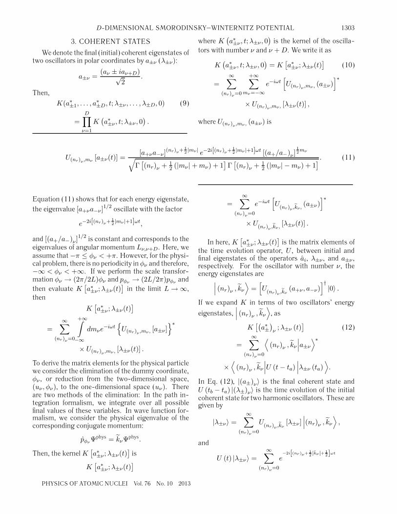
where U(nr)ν ,mν , (a±ν) is

U(nr)ν ,mν[a±ν(t)] =

[a+νa−ν ](nr)ν+ 1

2|mν | e−2i[(nr)ν+ 1

2|mν |+1]ωt [(a+/a−)ν ]

12mν

√Γ[(nr)ν + 1

2 (|mν | + mν) + 1]Γ[(nr)ν + 1

2 (|mν | − mν) + 1] . (11)

Equation (11) shows that for each energy eigenstate,the eigenvalue [a+νa−ν ]

1/2 oscillate with the factor

e−2i[(nr)ν+ 12|mν |+1]ωt,

and [(a+/a−)ν ]1/2 is constant and corresponds to the

eigenvalues of angular momentum Lν,ν+D. Here, weassume that −π ≤ φν < +π. However, for the physi-cal problem, there is no periodicity in φν and therefore,−∞ < φν < +∞. If we perform the scale transfor-mation φν → (2π/2L)φν and pφν → (2L/2π)pφν andthen evaluate K

[a∗±ν ;λ±ν(t)

]in the limit L → ∞,

then

K[a∗±ν ;λ±ν(t)

]

=∞∑

(nr)ν=0

+∞∫

−∞

dmνe−iωt

{U(nr)ν ,mν , [a±ν ]

}∗

× U(nr)ν ,mν , [λ±ν(t)] .

To derive the matrix elements for the physical particlewe consider the elimination of the dummy coordinate,φν , or reduction from the two-dimensional space,(uν , φν), to the one-dimensional space (uν). Thereare two methods of the elimination: In the path in-tegration formalism, we integrate over all possiblefinal values of these variables. In wave function for-malism, we consider the physical eigenvalue of thecorresponding conjugate momentum:

pφνΨphys = kνΨphys.

Then, the kernel K[a∗±ν ;λ±ν(t)

]is

K[a∗±ν ;λ±ν(t)

]

=∞∑

(nr)ν=0

e−iωt[U

(nr)ν ,kν ,(a±ν)

]∗

× U(nr)ν ,kν ,

[λ±ν(t)] .

In here, K[a∗±ν ;λ±ν(t)

]is the matrix elements of

the time evolution operator, U , between initial andfinal eigenstates of the operators ai, λ±ν , and a±ν ,respectively. For the oscillator with number ν, theenergy eigenstates are

∣∣∣ (nr)ν , kν

⟩=[U

(nr)ν ,kν(a+ν , a−ν)

]†|0〉 .

If we expand K in terms of two oscillators’ energy

eigenstates,∣∣∣ (nr)ν , kν

⟩, as

K[(

a∗±)ν;λ±ν (t)

](12)

=∞∑

(nr)ν=0

⟨(nr)ν , kν

∣∣∣a±ν

⟩∗

×⟨

(nr)ν , kν

∣∣∣U (t − ta)∣∣∣λ±ν (ta)

⟩.

In Eq. (12), |(a±)ν〉 is the final coherent state andU (tb − ta) |(λ±)ν〉 is the time evolution of the initialcoherent state for two harmonic oscillators. These aregiven by

|λ±ν〉 =∞∑

(nr)ν=0

U(nr)ν ,kν

[λ±ν ]∣∣∣(nr)ν , kν

⟩,

and

U (t) |λ±ν〉 =∞∑

(nr)ν=0

e−2i[(nr)ν+1

2 |kν |+ 12 ]ωt

PHYSICS OF ATOMIC NUCLEI Vol. 76 No. 10 2013

1304 NURI UNAL

× U(nr)ν ,kν

(λ±ν)∣∣∣(nr)ν , kν

⟩.

The coherent states are parametrized by D quantum

numbers,[(nr)ν + 1

2

∣∣∣kν

∣∣∣]

, ν = 1, 2, . . . ,D.

4. COHERENT STATESIN CONFIGURATION SPACE

4.1. Coherent States in Cartesian CoordinatesIn the previous section, we derive the kernel be-

tween the initial and final coherent states. However,in this section, we introduce a new kernel betweenthe configuration space eigenstates and the coherentstates for each set of harmonic oscillators as

Kν [uν , φν , t;λ±ν , 0] = Kν [uν , φν ;λ±ν(t)] (13)

=∫

da∗+da+da∗

−da−

(2πi)2e−a∗

+a+−a∗−a−

× 〈uν , φν |a+ν , a−ν〉Kν

[a∗±ν ;λ±ν (t)

].

The matrix elements, 〈uν , φν |a+ν , a−ν〉 can be calcu-lated by using the representations of a±ν in terms ofuν , φν , and puν , pφν , in Eq. (4). Since the volumeelement of the two-dimensional space is uνduνdφν ,the normalized wave functions will be

〈uν , φν |a+ν , a−ν〉

= Ne−Mωu2ν/2e

√Mωuν(a+νe−iφν +a−νeiφν )− 1

2a2

,

where a2 is defined asa2 = a2

+ + a2−,

and the normalization constant, N , is given as

N =(

Mω

π

)1/2

e−|λν |2/2.

If we substitute 〈uν , φν |a±ν〉 into Eq. (13) andintegrate over a∗±ν , a±ν , the result is

Kν [uν , φν ;λ±ν(t)] = Ne−iωte−Mωu2ν/2 (14)

× e√

Mω[uν(λ+νe−iφν +λ−νeiφν )]− 12λ2

ν ,

where we omit the time dependence of the λ±ν .In order to derive coherent states in polar coordi-

nates, we rewrite Eq. (13) as

Kν(uν , φν ;λ±ν) = Ne−iωte−Mωu2ν/2+(iλν)2 (15)

× e

√Mωu2

ν(−iλν)2

2

[(ei(φν−Δν+ π

2 )−e−i(φν−Δν+ π2 ))]

,

where the phase, Δν , is

λν + iλν+D =√

λ2ν exp iΔν .

Then, we can expand the kernel in terms of Besselfunctions as

Kν(uν , φν ;λ±ν) = Ne−iωte−Mω

�u2

ν/2−λ2ν (16)

×+∞∑

mν=−∞J|mν |

(−2i

√Mωu2

ν

λ2ν

2

)eimν(φν−Δν+ π

2 ).

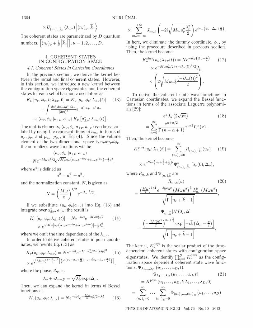
In here, we eliminate the dummy coordinate, φν , byusing the procedure described in previous section.Then, the kernel becomes

Kphysν (uν ;λ±ν(t)) = Ne−ikν(Δν−π

2 ) (17)

× e−Mωu2ν/2+(−iλν(t))2/2J

kν

×

⎛

⎝2

√

Mωu2ν

(−iλν(t))2

2

⎞

⎠ .

To derive the coherent state wave functions inCartesian coordinates, we expand the Bessel func-tions in terms of the associate Laguerre polynomi-als [29]:

ezJα

(2√

xz)

(18)

=∞∑

n=0

zn+α/2

Γ (n + α + 1)xα/2Lα

n (x) .

Then, the kernel becomes

Kphysν [uν ;λ± (t)] =

∞∑

(nr)ν=0

R(nr)ν ,kν

(uν) (19)

× e−2iω

(nr+ k

2+ 1

2

)tΨ∗

(nr)ν ,kν[λν(0),Δν ] ,

where Rnr ,k and Ψ(nr),k

are

Rnr,k(u) (20)

=

(Mωπ

)1/4e−

Mω2

u2 (Mωu2

) k2 Lk

nr

(Mωu2

)√

Γ[nr + k + 1

] ,

Ψnr ,k

[λ∗(0),Δ]

=

(− (λ∗(0))2

2

)nr+ k2 exp

[−ik

(Δν − π

2

)]

√Γ[nr + k + 1

] .

The kernel, Kphysν is the scalar product of the time-

dependent coherent states with configuration spaceeigenstates. We identify

∏Dν=1 K

physν as the config-

uration space dependent coherent state wave func-tions, Ψλ1,...,λD

(u1, . . . , uD, t):

Ψλ1,...,λD(u1, . . . , uD, t) (21)

= Kphys (u1, . . . , uD, t;λ1, . . . , λD, 0)

=∞∑

(nr)1=0

. . .

∞∑

(nr)D=0

Φ(nr)1,...,(nr)D(u1, . . . , uD)

PHYSICS OF ATOMIC NUCLEI Vol. 76 No. 10 2013

D-DIMENSIONAL SMORODINSKY–WINTERNITZ POTENTIAL 1305

× e−2iω[(nr)1+ ... +(nr)D+ 12(|k1|+ ...+|kD|)+ D

2 ]t

×[Ψ(nr)1,...,(nr)D

(λ1, . . . , λD)]∗

.

In Eq. (21),

Φ(nr)1,...,(nr)D(u1, . . . , uD) (22)

= (u1)1/4 R

(nr)1,k1(u1) · · ·

(u2

D

)1/4R

(nr)D,kD(uD),

Ψ(nr)1,...,(nr)D(λ∗

1, . . . , λ∗D)

= Ψ(nr)1,k1

[λ∗1(0),Δ1] · · ·Ψ(nr)D,kD

[λ∗D(0),ΔD ] ,

are the energy eigenstates in Cartesian coordinatesand holomorphic coordinates of D oscillators, re-spectively. Thus, for a particle in the potentialgiven by Eq. (1), Ψλ1,...,λD

(u1, . . . , uD, t) is thecoherent state and it is given in terms of the nor-malized energy eigenstates in Cartesian coordinates,Φ(nr)1,...,(nr)D

(u1, . . . , uD).

4.2. Coherent States in Hyperspherical Coordinates

Cartesian coordinates, (u1, . . . , uD) are relatedinto hyperspherical coordinates (r, θ1, . . . , θD−1) bythe following relations:

u1 = r sin θ1 · · · sin θD−1, (23)

uν = r sin θ1 · · · cos θD−ν+1, ν = 2, . . . ,D.

Similarly, we introduce hyperspherical coordinates for(λ1, . . . , λD) as (Λ,Θ1, . . . ,ΘD−1)

λ1 = Λsin Θ1 · · · sinΘD−1, (24)

λν = Λsin Θ1 · · · cos ΘD−ν+1, ν = 2, . . . ,D.

In order to find the coherent state wave functions inhyperspherical coordinates, we write the product oftwo modified Bessel functions in terms of one mod-ified Bessel function [30]:

z

2Jμ (z sin α sinβ) Jν (z cos α cos β)

= (sin α sin β)μ (cos α cos β)ν∞∑

l=0

N(μ,ν)l

× Jμ+ν+2l+1 (z) P(μ,ν)l (cos 2α) P

(μ,ν)l (cos 2β) ,

where the constant, N(μ,ν)l , is

N(μ,ν)l =

i (−1)l l!Γ (μ + ν + l + 1)Γ (μ + l + 1) Γ (ν + l + 1)

.

We parametrize the product of two modified Besselfunctions as

Jk1

⎛

⎝2

√

Mωu21

[−λ2

1

]

2

⎞

⎠Jk2

⎛

⎝2

√

Mωu22

[−λ2

2

]

2

⎞

⎠

= Jk1

(2ξ1 sin θD−1 sin ΘD−1)

× Jk2

(−2iξ1 cos θD−1 cos ΘD−1) ,

where

u2 + iu1 =√

u21 + u2

2 exp iθD−1,

λ2 + iλ1 =√

λ21 + λ2

2 exp iΘD−1,

ξ1 =

√

Mω(u2

1 + u22

)[−(λ2

1 + λ22

)]

2.

Then, we combine Jk1

and Jk2

as

Jk1

(−2iξ1 sin θD−1 sin ΘD−1)

× Jk2

(−2iξ1 cos θD−1 cos ΘD−1)

=∞∑

l1=0

N(k1,k2)l1

J2l1+k1+k2+1

(−2iξ1)

ξ1

× dl1k1,k2

(cos 2θD−1)dl1k1,k2

(cos 2ΘD−1),

where the angular wave functions dl1,k1,k2

(cos 2θD−1)are defined in terms of Jacobi polynomials,

P(k1,k2)l1

(cos 2θD−1), as

dl1k1,k2

(cos 2θD−1) = (sin θD−1)k1

× (cos θD−1)k2 P

(k1,k2)l1

(cos 2θD−1) .

In the similar way, we write uν+1 and λν+1 as

uν+1 =√

u21 + . . . + u2

ν cos θD−ν,

and λν+1 =√

λ21 + . . . + λ2

ν cos ΘD−ν .

We express ξν in terms of ξν+1 as

ξν = ξν+1 sin θD−(ν+1) sin ΘD−(ν+1) =

√Mω

2(u2

1 + . . . + u2ν+1

) [−(λ2

1 + . . . + λ2ν+1

)].

PHYSICS OF ATOMIC NUCLEI Vol. 76 No. 10 2013

1306 NURI UNAL

Then, similarly, we combine

J2l1+k1+k2+1

(2ξ2 sin θD−2 sin ΘD−2) Jk3

(2ξ2 cos θD−2 cos ΘD−2)

ξ1

=∞∑

l2=0

N(2l1+k1+k2+1,k3)l2

J2l2+2l1+k1+k2+2

(2ξ2)

ξ1ξ2

× dl22l1+k1+k2+1,k3

(cos 2θD−2)dl22l1+k1+k2+1,k3

(cos 2ΘD−2).

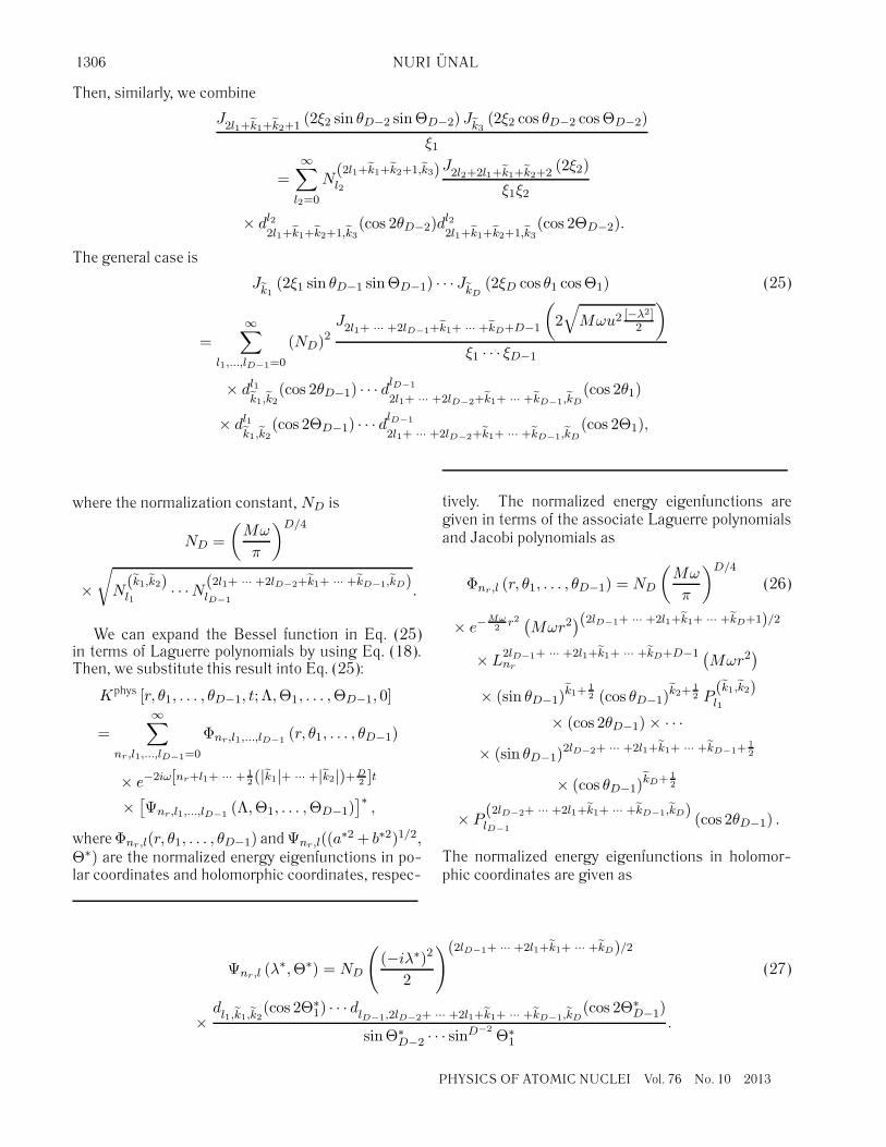
The general case is

Jk1

(2ξ1 sin θD−1 sinΘD−1) · · · JkD(2ξD cos θ1 cos Θ1) (25)

=∞∑

l1,...,lD−1=0

(ND)2J

2l1+ ··· +2lD−1+k1+ ··· +kD+D−1

(2√

Mωu2 [−λ2]2

)

ξ1 · · · ξD−1

× dl1k1,k2

(cos 2θD−1) · · · dlD−1

2l1+ ··· +2lD−2+k1+ ··· +kD−1,kD(cos 2θ1)

× dl1k1,k2

(cos 2ΘD−1) · · · dlD−1

2l1+ ··· +2lD−2+k1+ ··· +kD−1,kD(cos 2Θ1),

where the normalization constant, ND is

ND =(

Mω

π

)D/4

×√

N(k1,k2)l1

· · ·N(2l1+ ··· +2lD−2+k1+ ··· +kD−1,kD)lD−1

.

We can expand the Bessel function in Eq. (25)in terms of Laguerre polynomials by using Eq. (18).Then, we substitute this result into Eq. (25):

Kphys [r, θ1, . . . , θD−1, t; Λ,Θ1, . . . ,ΘD−1, 0]

=∞∑

nr ,l1,...,lD−1=0

Φnr,l1,...,lD−1(r, θ1, . . . , θD−1)

× e−2iω[nr+l1+ ··· + 12(|k1|+ ··· +|k2|)+ D

2 ]t

×[Ψnr,l1,...,lD−1

(Λ,Θ1, . . . ,ΘD−1)]∗

,

where Φnr,l(r, θ1, . . . , θD−1) and Ψnr,l((a∗2 + b∗2)1/2,Θ∗) are the normalized energy eigenfunctions in po-lar coordinates and holomorphic coordinates, respec-

tively. The normalized energy eigenfunctions aregiven in terms of the associate Laguerre polynomialsand Jacobi polynomials as

Φnr ,l (r, θ1, . . . , θD−1) = ND

(Mω

π

)D/4

(26)

× e−Mω2

r2 (Mωr2

)(2lD−1+ ··· +2l1+k1+ ··· +kD+1)/2

× L2lD−1+ ··· +2l1+k1+ ··· +kD+D−1nr

(Mωr2

)

× (sin θD−1)k1+

12 (cos θD−1)

k2+ 12 P

(k1,k2)l1

× (cos 2θD−1) × · · ·

× (sin θD−1)2lD−2+ ··· +2l1+k1+ ··· +kD−1+

12

× (cos θD−1)kD+ 1

2

× P(2lD−2+ ··· +2l1+k1+ ··· +kD−1,kD)lD−1

(cos 2θD−1) .

The normalized energy eigenfunctions in holomor-phic coordinates are given as

Ψnr,l (λ∗,Θ∗) = ND

((−iλ∗)2

2

)(2lD−1+ ··· +2l1+k1+ ··· +kD)/2

(27)

×d

l1,k1,k2(cos 2Θ∗

1) · · · dlD−1,2lD−2+ ··· +2l1+k1+ ··· +kD−1,kD(cos 2Θ∗

D−1)

sinΘ∗D−2 · · · sinD−2 Θ∗

1

.

PHYSICS OF ATOMIC NUCLEI Vol. 76 No. 10 2013

D-DIMENSIONAL SMORODINSKY–WINTERNITZ POTENTIAL 1307

The energy eigenstates in Eq. (26) are in agreementwith [18].

5. CONCLUSION

In this study, we solved the quantum equationsfor a particle in the D-dimensional Smorodinsky–Winternitz potentials and derived the coherent statesand energy eigenstates of the system. We first trans-formed the system into a particle in 2D-dimensionalharmonic oscillator potential and derived the evolu-tion of the coherent states for this new system. Sec-ond, the coherent states of D-dimensional originalsystem is derived by dimensional reduction. Third,in the Cartesian and hyperspherical coordinates, weobtained the stationary states of a particle in D-dimensional Smorodinsky–Winternitz potentials byexpanding the time-dependent coherent states intothe power series of raising operators of the system.

ACKNOWLEDGMENTS

This work was supported by Akdeniz University,Scientific Research Projects Unit.

REFERENCES1. W. Pauli, Z. Phys. 36, 336 (1926).2. V. Fock, Z. Phys. 98, 145 (1935).3. V. Bargmann, Z. Phys. 99, 576 (1936).4. J. M. Jauch and E. L. Hill, Phys. Rev. 57, 641 (1940).5. M. Moshinsky and Yu. F. Smirnov, Contemporary

Concepts in Physics, Vol. 9 (Harwood, Amsterdam,1996).

6. I. Fris, V. Mandrosov, Ya. A. Smorodinsky, et al.,Phys. Lett. 16, 354 (1965).

7. P. Winternitz, Ya. A. Smorodinsky, M. Uhlir, andI. Fris, Sov. J. Nucl. Phys. 4, 444 (1967) [Yad. Fiz.4, 625 (1966)].

8. A. A. Makarov, Ya. A. Smorodinsky, Kh. Valiev, andP. Winternitz, Nuovo Cimento A 52, 1061 (1967).

9. N. W. Evans, Phys. Rev. A 41, 5666 (1990).10. E. G. Kalnins, J. M. Kress, and W. Miller, J. Math.

Phys. 46, 053509 (2005).11. E. G. Kalnins, J. M. Kress, and W. Miller, J. Math.

Phys. 46, 053510 (2005).12. E. G. Kalnins, J. M. Kress, and W. Miller, J. Math.

Phys. 46, 103507 (2005).13. E. G. Kalnins, J. M. Kress, and W. Miller, J. Math.

Phys. 47, 043514 (2006).14. E. G. Kalnins, J. M. Kress, and W. Miller, J. Math.

Phys. 47, 093501 (2006).15. C. Daskaloyannis and K. Ypsilantis, J. Math. Phys.

47, 042904 (2006).16. C. Daskaloyannis and Y. Tanoudis, J. Math. Phys. 48,

072108 (2007).17. C. Grosche, G. S. Pogosyan, and A. N. Sissakian,

Fortschr. Phys. 43, 453 (1995).18. C. Quesno, SIGMA 7, 035 (2011).19. E. Schrodinger, Naturwissenschaften 14, 664 (1926).20. R. J. Glauber, Phys. Rev. Lett. 10, 84 (1963); Phys.

Rev. 130, 2529 (1963).21. M. M. Nieto and L. M. Simmons, Jr., Phys. Rev. Lett.

41, 207 (1978).22. L. S. Brown, Am. J. Phys. 41, 525 (1973).

23. N. Unal, Found Phys. 28, 755 (1998).

24. N. Unal, Phys. Rev. A 63, 052105 (2001); Turk.J. Phys. 24, 463 (2000).

25. N. Unal, Can. J. Phys. 80, 875 (2002).

26. N. Unal, in Fluctuating Paths and Fields, Ed. byW. Janke et al. (World Sci., Singapore, 2001).

27. N. Unal, J. Math. Phys. 47, 122105 (2006).

28. N. Unal, J. Math. Phys. 48, 122107 (2007); Cent.Eur. J. Phys. 7, 774 (2009); Phys. Atom. Nucl. 74,1758 (2011) [Yad. Fiz. 74, 1796 (2011)].

29. I. S. Gradshteyn and I. M. Ryzhik, Table of Inte-grals, Series, and Products (Academic Press, NewYork, 1980).

30. G. N. Watson, Theory of Bessel Functions (Cam-bridge Univ. Press, London, 1922).

PHYSICS OF ATOMIC NUCLEI Vol. 76 No. 10 2013