ADEM A278 463 A F"ORTRAN 13ASED LEARNING SYSTEM USING MULTILAYER BACK- PROPAGATION NEURAL NETWORK TECHNIQUES THlES IS Gregory L. Reinhart C~aptain, USAF D I AFIT/GOR/ENS/94M-11 ELECT APR 2 21994 DEPARTMENT OF THE AIR FORCE DTICQUALITYflSMPC'rED AIR UNIVERSITY AIR FORCE INSTITUTE OF TECHNOLOGY Wright-Patterson Air Force Base, Ohio
Transcript
ADEM A278 463
A F"ORTRAN 13ASED LEARNING SYSTEM USING
MULTILAYER BACK- PROPAGATION
NEURAL NETWORK TECHNIQUES
THlES ISGregory L. Reinhart
C~aptain, USAF D IAFIT/GOR/ENS/94M-11 ELECT
APR 2 21994
DEPARTMENT OF THE AIR FORCE DTICQUALITYflSMPC'rEDAIR UNIVERSITY
a Ability to monitor change in weights between network nodes while the network was
training. The specific weights to monitor would be user defined and would be reported
after each epoch.
* Ability to interrupt network training to see the "status" of the neural network.
* After analyzing the "status" of the network, decide whether to continue training the
network or to quit training and report on final results.
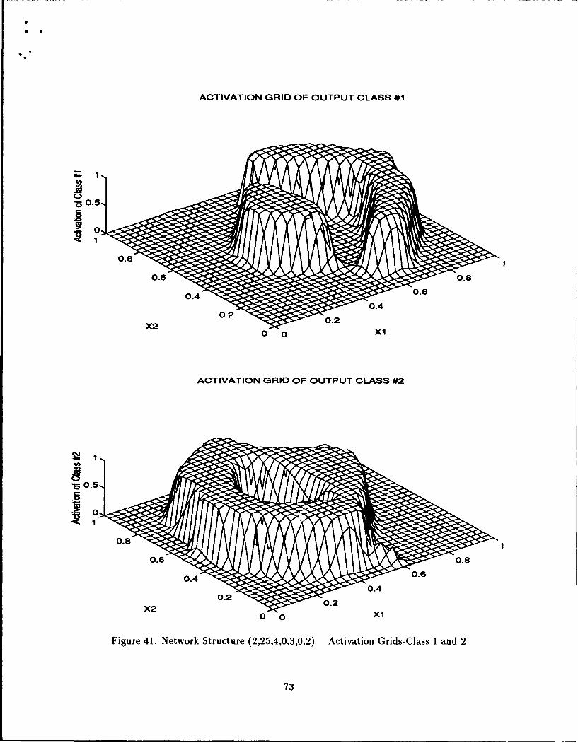
* After network is trained, produce 2D graphs of historical output errors, classification
errors, and user requested weights. Also produce 3D graphs of network activations
and saliencies as specified by the user. All 3D graphs will have the ability to rotate
to any view in an interactive mode and then be printed.
"* Reduce the number of random numbers required to run the network.
"* Increase computer storage efficiency in order to handle larger networks and data sets.
"* Interface a sort algorithm into the current FORTRAN program to improve the effi-
ciency of reshuffling the training and test sets after each epoch.
1.3 Scope
FORTRAN software developed by Belue for her thesis titled An Investigation of
Multilayer Perceptrons for Classification provided an excellent program shell from which
to begin the revisions and extensions [1]. In addition, subroutines developed by Steppe for
her dissertation titled Feature Selection in Feedforward Neural Networks were incorporated
into the main body of the software [18].
In order to revise and incorporate new procedures into the existing software, a thor-
ough study of the underlying concepts of multilayer back-propagation and feature saliency
was required. In addition, the logic and program flow of the existing software had to be
analyzed and thoroughly understood. The next step was to develop an interface between
FORTRAN and MATLAB that would allow the user to "jump" between the two languages
as often and whenever the user desired, while still maintaining network training integrity.
All throughout this process, a constant eye was kept on ways to improve computational
efficiency and ways to shrink data storage requirements. Finally, graphs, output reports,
5
and raw data files had to be designed to display the volumes of data produced by the
program.
6
II. Literature Review
This chapter provides a review of the literature concerning multilayer back-prop-
agation neural networks, the saliency metric, and sort algorithms. Specifically, it will
define terms peculiar to the neural network field, describe the multilayer back-propagation
algorithm, define the concept of saliency and its calculation, describe high-order inputs
and their relation to correlation matrices, and finish with a discussion on the Shell-Mezgar
sort algorithm. The intent is to give the reader a feel for why things were calculated the
way they were in the FORTRAN code and why the parameter file is designed the way it
is. See Appendix A for an example of the parameter file.
2.1 Terms Defined
As in many other fields of science, neural networks have their own brand of termi-
nology. Several basic terms related to this field are defined below.
"* Back-propagation A learning algorithm for updating weights in a multilayer, feed-
forward, mapping neural network that minimizes mean squared mapping error [4].
"* Classifier The decision making system built by the neural network. In a sense, the
final set of weights.
"* Epoch A complete presentation of the data set being used to train the niultilayer
perceptron, also called a training cycle.
"* Exemplar The input data to a neural network is a finite set of solved cases. Each
case is known as an exemplar or input vector.
"• Feature The individual measurements found in exemplars which contain information
useful for distinguishing the various classes. In other fields, features are known as
attributes or independent variables.
"* Feedforward Characterized by multilayer neural networks whose connections ex-
clusively feed inputs from lower to higher layers; in contrast to a feedback network,
a feedforward network operates only until its inputs propagate to its output layer.
An example of a feedforward neural network is the multilayer perceptron [4].
7
"* Hidden Units Those processing elements in multilayer neural network architectures
which are neither the input layer nor the output layer, but are located in between
these and allow the network to undertake more complex problem solving [4].
"* Learning Algoithms In neural networks, the equations which modify some of the
weights of processing elements in response to input and output values [4].
"* Multilayer Perceptron A multilayer feedforward network that is fully connected
and which is typically trained by the back-propagation learning algorithm [4].
"* Neural Network An information processing system which operates on inputs to
extract information and produces outputs corresponding to the extracted information
[4].
"* Single-layer Perceptron A type of neural network algorithm used in pattern clas-
sification problems and trained with supervision. Connection weights and thresholds
in a perceptron can be fixed or adapted using a number of different algorithms [4].
"* Supervised Training A means of training adaptive neural networks which requires
labeled training data and an external teacher. The teacher knows the correct response
and provides an error signal when an error is made by the network [4].
"* Weight A processing element (or neuron or unit) need not treat all inputs uni-
formly. Processing elements receive inputs by means of interconnects (also called
'connections' or 'links'); each of these connections has an associated weight which
signifies its strength. The weights are combined to calculate the activations [4].
2.2 Error Rates
The overall objective of building a classifier is to learn from samples and to generalize
to new, as yet unseen cases. Performance is most easily and directly measured in terms
of the error rate, which is the ratio of the number of errors to the number of samples or
cases.number of errorserror rate =(1number of cases
8
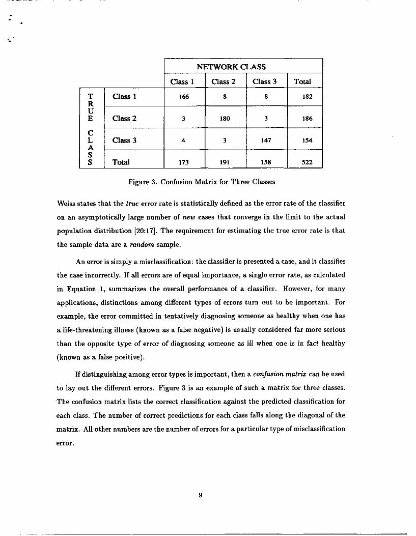
NETWORK CLASS
Class 1 Class 2 Class 3 Total
T Class 1 166 8 8 182RUE Class 2 3 180 3 186
CL Class 3 4 3 147 154AS
S Total 173 191 158 522
Figure 3. Confusion Matrix for Three Classes
Weiss states that the true error rate is statistically defined as the error rate of the classifier
on an asymptotically large number of new cases that converge in the limit to the actual
population distribution [20:171. The requirement for estimating the true error rate is that
the sample data are a random sample.
An error is simply a misclassification: the classifier is presented a case, and it classifies
the case incorrectly. If all errors are of equal importance, a single error rate, as calculated
in Equation 1, summarizes the overall performance of a classifier. However, for many
applications, distinctions among different types of errors turn out to be important. For
example, the error committed in tentatively diagnosing someone as healthy when one has
a life-threatening illness (known as a false negative) is usually considered far more serious
than the opposite type of error of diagnosing someone as ill when one is in fact healthy
(known as a false positive).
If distinguishing among error types is important, then a confusion matrix can be used
to lay out the different errors. Figure 3 is an example of such a matrix for three classes.
The confusion matrix lists the correct classification against the predicted classification for
each class. The number of correct predictions for each class falls along the diagonal of the
matrix. All other numbers are the number of errors for a particular type of misclassification
error.
9
The apparent error rate of a classifier is the error rate of the classifier on the sample
cases that were used to design or build the classifier. Since we are trying to extrapolate
performance from a finite sample of cases, the apparent error rate is the obvious starting
point in estimating the performance of a classifier on new cases. For most types of classi-
fiers, the apparent error rate is a poor estimator of future performance. Lippmann believes
that in general, apparent error rates tend to be biased optimistically. The true error rate
is almost invariably higher than the apparent error rate. This happens when the classifier
has been overfitted (or overspecialized) to the particular characteristics of the sample data
[10].
It is useless to design a classifier that does well on the design sample data, but
does poorly on new cases. And unfortunately, using solely the apparent error to estimate
future performance can often lead to disastrous results on new data. Many a learning
system designer has been lulled into a false sense of security by the mirage of favorably
low apparent error rates [20:25].
2.3 Training vs Test vs Validation Set
Instead of using all the cases to estimate the true error rate, the cases can be parti-
tioned into three sets [7:115-117]. The first set is used to design the classifier, the second
to test the classifier, and the third to validate the classifier.
" The Training Set: This set is used to design or train the weights in the multilayer
perceptron. Foley's Rule [5] provides some guidelines as to the minimum number
of training vectors required for accurate classification as a function of the number
of input features. Foley showed empirically that the number of training samples per
class should be greater than three times the number of features.
" The Test Set: This set is used to test the accuracy of training while training is
ongoing. After each epoch, the test set acts as a barometer for determining when
the accuracy of the perceptron is at an acceptable level.
10
* The Validation Set: After the multilayer perceptron is considered optimally trained,
the validation set is presented to the classifier. It verifies the performance of the clas-
sifier since its exemplars are never seen by the classifier during its development.
2.4 Multilayer Perceptrons
This section will use a building block approach to define the algorithm used in multi-
layer back-propagation. It starts out with the idea of a linear discriminant, then graduates
to the concepts of single output perceptron, learning rate, multilayer perceptron, back-
propagation, and finally, the concept of momentum.
2.4.1 Linear Discriminants. Linear discriminants are the most common form of
classifier, and are quite simple in structure. The name linear discriminant simply indicates
that a linear combination of the evidence will be used to separate or discriminate among
the classes and to select the class assignment for a new case. For a problem involving n
features, this means geometrically that the separating surface between the samples will
be an (n - 1) dimensional hyperplane [10]. In most situations, classes can overlap and
therefore cannot be completely separated by a plane (or line in two dimensions). The
classic example of this is the logical "exclusive or (XOR)" problem.
Equation 2 gives the general form for any linear discriminant,
wIX1 + w2X2 +...-- + wXn - WO (2)
where (x 1 , X2,... , x,) are the usual list or vector of n features, and wi are constants that
must be estimated. A linear discriminant simply implements a weighted sum of the values
of the observations. Intuitively, we can think of the linear discriminant as a scoring function
that adds to or subtracts from each observation, weighing some observations more than
others and yielding a final total score. The class selected, Ci, is the one with the highest
score.
2.4.2 Single-Output Perceptron. The simplest neural net device is the single-
output perceptron. More complex neural networks can be described as combinations of
11
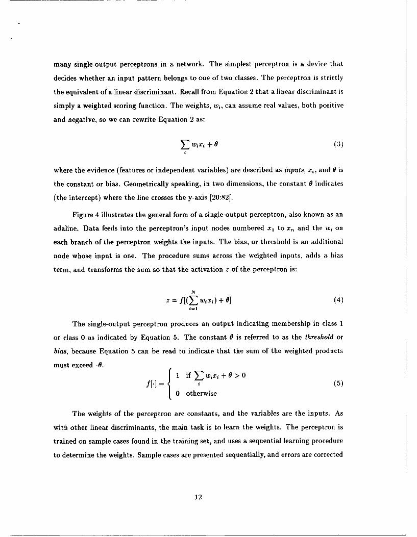
many single-output perceptrons in a network. The simplest perceptron is a device that
decides whether an input pattern belongs to one of two classes. The perceptron is strictly
the equivalent of a linear discriminant. Recall from Equation 2 that a linear discriniinant is
simply a weighted scoring function. The weights, w,, can assume real values, both positive
and negative, so we can rewrite Equation 2 as:
jw x, + 0 (:)
where the evidence (features or independent variables) are described as inputs, xj, and 0 is
the constant or bias. Geometrically speaking, in two dimensions, the constant 0 indicates
(the intercept) where the line crosses the y-axis [20:821.
Figure 4 illustrates the general form of a single-output perceptron, also known as an
adaline. Data feeds into the perceptron's input nodes numbered x, to x,, and the wi on
each branch of the perceptron weights the inputs. The bias, or threshold is an additional
node whose input is one. The procedure sums across the weighted inputs, adds a bias
term, and transforms the sum so that the activation z of the perceptron is:
Nz = f EWix) + 0] (4)i=1
The single-output perceptron produces an output indicating membership in class 1
or class 0 as indicated by Equation 5. The constant 0 is referred to as the threshold or
bias, because Equation 5 can be read to indicate that the sum of the weighted products
must exceed -0.
= f1 if Ewix:+0>0f[] (5)
0 otherwise
The weights of the perceptron are constants, and the variables are the inputs. As
with other linear discriminants, the main task is to learn the weights. The perceptron is
trained on sample cases found in the training set, and uses a sequential learning procedure
to determine the weights. Sample cases are presented sequentially, and errors are corrected
12
z=f[(I wixi)+ 0]
+1
w R
x x x1 2 2
Figure 4. Single-Output Perceptron
by adjusting the weights after each erroneous output. If the perceptron output matches
the desired or true output, the weights are not adjusted.
Equation 6 describes the general form of an iterative procedure that adjusts the
weights. A sample is presented to the perceptron. Each new weight is computed by adding
a correction to the old weight. We describe the current weight as wi(t), the weight at time
t. The new weight is wi(t + 1), which will be the current weight at time t + 1. The new
weight wi(t-+ 1) is computed by adding an adjustment factor, Awi(t) to the current weight
wi(t). The threshold 0(t) is also revised.
wi(t + 1) = wi(t) + Awi(t) (6)
0(t + 1) = 0(t) + AO(t)
The task of the training procedure is to find Awi, the adjustment to any weight wi.
The training procedure for perceptrons is given in Equation 7, where d is the desired or
true answer, f[-] is the perceptron output, and xi is the perceptron input.
Awi(t) = (d-f[-])xi (7)
AO(t) = (d-f[.])
13
When a case is presented to the perceptron and the output is correct, no change is
made to any of the weights. If the output is incorrect, each weight is adjusted by adding or
subtracting the corresponding value in the input pattern. The hope is that each adjustment
will move the weights closer to the true weights.
2.4.3 The Learning Rate. While the perceptron convergence theorem, proved by
Rosenblatt, states that for linearly separable data the perceptron will eventually converge,
the speed with which the training will be completed is not known [15]. One may have to
wait a very long time for an answer. The perceptron will not necessarily get closer and
closer to the answer after each epoch. However, there are a number of modifications to
the data and the training procedures that may speed up learning and convergence. Two
of the most important are:
1. Normalize the data: Performance is often improved by normalizing the data between0 and 1, or by using Gaussian normalization.
2. Make the learning rate adjustable by introducing a learning rate parameter, q in theperceptron weight updating procedure. Instead of using Awi as the correction factor,we use i7Awi, where q1 is usually chnsen between 0 and 1.
Weiss states that, while these measures can improve the rate of convergence, there is
no way of knowing in advance the value of the learning rate that will speed up convergence
the most for a specific data set. He adds that, if the learning rate is too large, training
may not converge and just oscillate between wrong answers. Or, it may converge to a local
minimum [20:86-90]. Equation 7, when modified to incorporate a learning rat'- term, 77,
becomes Equation 8. As we shall see later in this chapter, Equation 8 will be used in the
training procedures for more complicated neural nets.
Awi(t) = 77(d- f[.])x, (8)
AO(t) = 7j(d- f[-])
The perceptron cannot train correctly when the classes are not linearly separable. In
addition, very few real-world applications are truly linearly separable. Hence, relying on
the predictive potential of linear solutions has troubled many researchers because it is easy
to come up with counter-examples of simple data sets that cannot be separated by lines.
14
The most commonly cited example comes from applying the "exclusive or" XOR, logical
operator on two binary features. A very similar learning system that fits a line, but is less
dependent on linear separability for good results, is discussed in the next section.
2.4.4 Least Mean Square Learning System. The least mean square learning
system, known simply as LMS, is another system that finds linear solutions. The only
functional difference is in the way the output, f[.1, is computed. The LMS system uses
the actual net output without any further mapping into 0 or 1. For a given input, the
output of the LMS device is simply the product of the inputs and weights summed with
the threshold.
f[.] = wjx, + 0 (9)
For the LMS learning system, the correct answers are still expressed as 0 or 1, but the
output is now a real number.
The goal of the LMS training procedure is to minimize the average squared distance
from the true answer to the net output. This is equivalent to finding a set of weights and
a threshold that minimize:
-(d, fj[.]) 2 (10)
Where j ranges over the number of samples in the training set.
It should be noted that the LMS training procedure does not directly reduce the
classification error rate. Rather, it reduces the distance between the output and the true
answer. Weiss states that reducing this distance is usually strongly related to reducing
classification error rates. However, it is quite possible that the classification error rate can
be relatively high even with a relatively small error distance. The error distances for the
correct answers may be quite small, while the erroneous answers may barely be on the
other side of the boundary [20:89].
2.4.5 Multilayer Perceptrons. The single-output perceptron and LMS learning
systems of the previous sections can be naturally extended to more complicated neural
networks. For example, the outputs of several perceptrons could be used as input to
15
other perceptrons. These devices could then be chained together ill many different ways.
Figure 5 illustrates the general structure of a multilayer network structure.
The perceptron can be described as a single-layer neural network, where a layer
represents a set of output devices. The network of Figure 5 is a two-layer network. Input
nodes are not counted as a layer. The inputs are connected to the first layer of outputs.
These outputs serve as inputs to the second layer of outputs. This is a fully connected
network; since every node serves as input to nodes in the next layer above.
The multilayer neural network has multiple outputs and multiple layers of outputs.
The final layer of outputs contains the decision results, called output units. The output
units of the intermediate layers are referred to as hidden units because they are not units
that are naturally defined by the application. Like the perceptron, each output unit has a
threshold or bias associated with it.
The multilayer network of Figure 5 can be extended to unlimited numbers of ad-
ditional layers. Potentially, this makes the multilayer neural network a very powerful
classifier. Cybenko has shown that, a two-layer network with one layer of hidden units,
can implement most decision surfaces, and can closely approximate any decision surface
[3]. In addition, this two-layer structure allows for the formation of nonlinear decision
regions, including disjoint regions. Therefore, this two-layer network structure is used in
the FORTRAN program developed in this research.
2.4.6 Back-Propagation Procedure. The multilayer neural net can be trained by
using the back-propagation training procedure. Before we discuss this procedure, a slight
variation in the computation of the output f[.], must be considered.
In the previously described perceptron, once the weighted sum was computed, the
activation of the output unit was determined by threshold logic. The activation f[.], was
0 or 1, depending on whether a threshold was exceeded. This threshold logic activation
function creates a nonlinearity, a desirable characteristic. However, it does not provide the
other desirable characteristic which we seek; that of a continuously differentiable function
[11]. In order to obtain these two characteristics, an alternative activation function, f[.],
is used; it is known as the sigmoidal or logistic function. For any real-valued numbers,
16
NETWORK
2 2 2
... Outputs
WA
Iz.
... HiddenLayer
S• +1win
W.0
x1 x2 x. +1 Inputs
Figure 5. Multilayer Network Structure
DETAIL OF HIDDEN LAYER NODE (m=2) DETAIL OF OUTPUT LAYER NODE (k=--)
whem N.: (ZWXI)+ 0 : - whee N,= N w,.;)+
02
I 2
e0,
+1 +1
,IJg X' w..2 I
23 2 212 2e
Figure 6. Detail of Hidden Layer and Output Layer Nodes
17
the output of the sigmoidal function is between 0 and 1. This function and its graph are
shown in Equation 11 and Figure 7.
1f(a) + (11)
-3 -2 -1 0 1 2 3S
Figure 7. Nonlinear Sigmoid Function
Equations 12 and 13 show how each training vector is propagated up through the
network to produce network outpuLs zM1 and zk. Equations 14 and 15 show how the
network outputs are then back-propagated down through the network, producing error
derivatives 61 and bJ. These error derivatives are then used to adjust the weights. After
the weights have been adjusted, the next training vector is presented and the process is
repeated. These equations are the heart of the back-propagation training procedure.
In Equation 12 the output or activation, z, , of a hidden unit, m, is computed by
applying a sigmoidal function to the net input, Nm, of unit m. The net input of hidden
unit m is the sum of the bias of hidden unit m, 01,,,, and the weighted sum of the input
features, xj, connected to hidden unit m. The weight, w!, connects input node j to hidden
node m. Refer to Figure 6 (Detail of Hidden Layer Node).
n
Nm = m X1 (11j=1 (12)
Zm . l+e N-
18
In Equation 13 the output or activation z4, of an output unit, k, is computed by applying
a sigmoidal function to the net input, Nk, of output unit k. The net input of output unit
k is the sum of the bias of unit k, 6k, and the weighted sum of the hidden layer outputs,
zi, connected to output unit k. The weight, wk connects hidden node j to output node k.
Nk E-- i iN--, W(13)
Z2 1
Equation 14 begins the error back-propagation by calculating the error derivative,
62, associated with output unit k:
b = z2(1 - Z)(dk- k) (14)
where z2 is the output of output unit k, and dk is the desired or true output of output unit
k. In Equation 15 the error derivative of hidden unit j, bJ1 is calculated by:
--z •2k wjk (15)k
where z• is the output of hidden unit j, 6b is the error derivative calculated in Equation 14,
and w?, is the weight connecting hidden unit j to output unit k.
We now have all the information required to calculate the new weights at time (t+ 1)
from the current weights at time t. Using Equations 6 and 8:
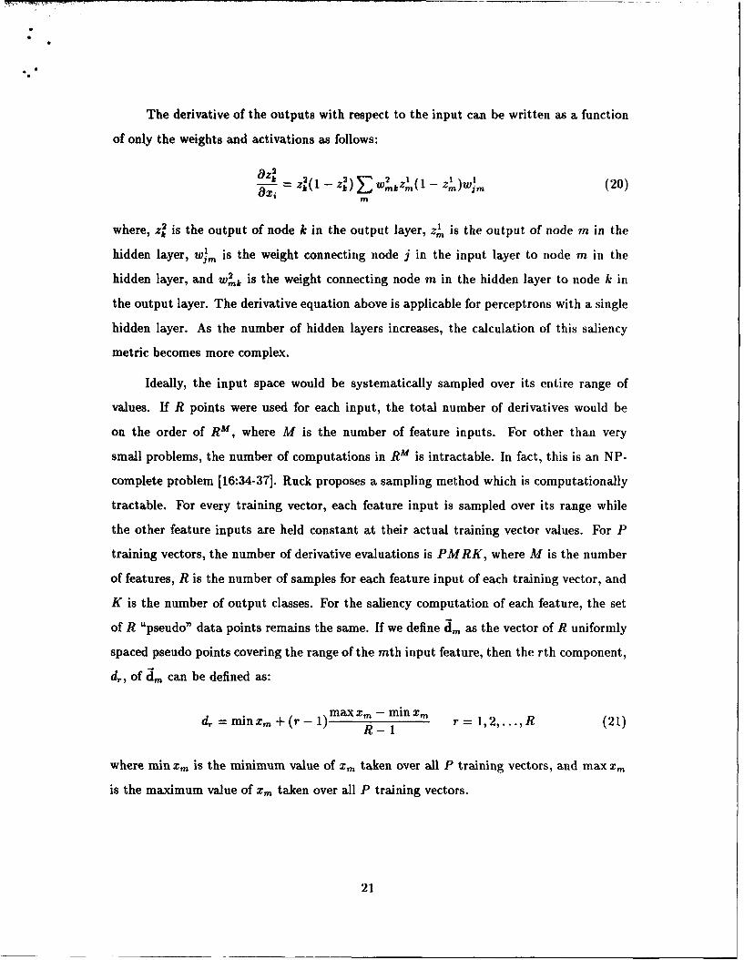
where minxm, is the minimum value of x.. taken over all P training vectors, and max xm
is the maximum value of xm taken over all P training vectors.
21
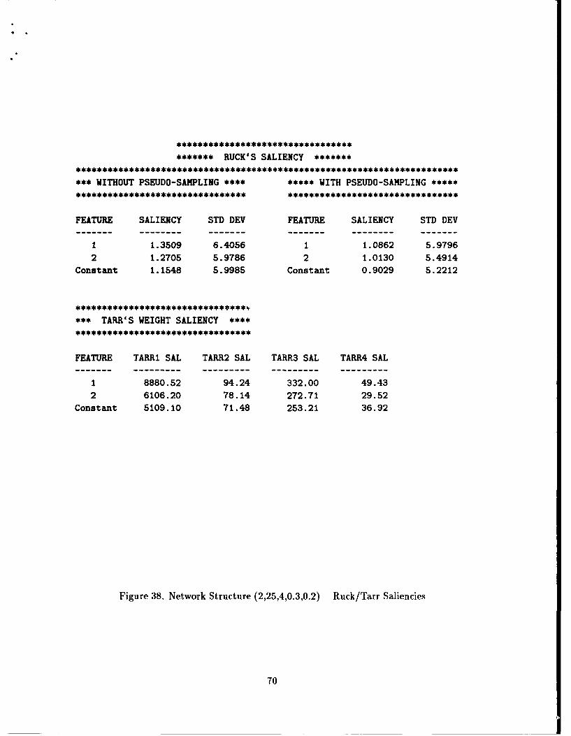
The Ruck saliency metric, Ai, for feature i when a sigmoid nonlinearity is used is
defined as:P M R K O2
X P (22)p1l iai1 r=I k-I (•X-'-i X f
where P is the number of training vectors i; M is the number of features; R is the number
of uniformly spaced points covering the range of each input feature found in the training
set; K is the number of output classes; the vector i(r) is the vector '4p with its mth
component replaced by, dr, the rth component of din; and (.-(r),i) indicates that the
derivative is evaluated with the feature vector j(r) and the final estimates of the trained
network weight parameters W. Also, the absolute value of the derivative is used, so positive
and negative derivative changes do not cancel out.
Equation 22 has been modified from Ruck's original presentation to reflect that for
each vector there are PMRK derivative evaluations as Ruck intended, rather than just
PRK derivative evaluations as denoted in Ruck's notation [16:37].
2.5.2 Tarr's Saliency. A simpler method of determining the relative significance
of the input features once the network has been trained has been suggested by Tarr. He
states the following:
When a weight is updated, the network moves the weight a small amountbased on the error. Given that a particular feature is relevant to the problemsolution, the weight would be moved in a constant direction until a solutionwith no error is reached. If the error term is consistent, the direction of themovement of the weight vector, which forms a hyper-plane decision boundary,will also be consistent. ... If the error term is not consistent, which can be thecase on a single feature out of the input vector, the movement of the weightattached to the node will also be inconsistent. In a similar fashion, if the featuredid not contribute to a solution, the weight updates would be random. In otherwords, useful features would cause the weights to grow, while weights attachedto non-salient features would simply fluctuate around zero. [19:44]
Therefore, the following alternate saliency metric is proposed:
rw= (W 2 (23)
Which is simply the sum of the squared weights between input node i and hidden node m.
22
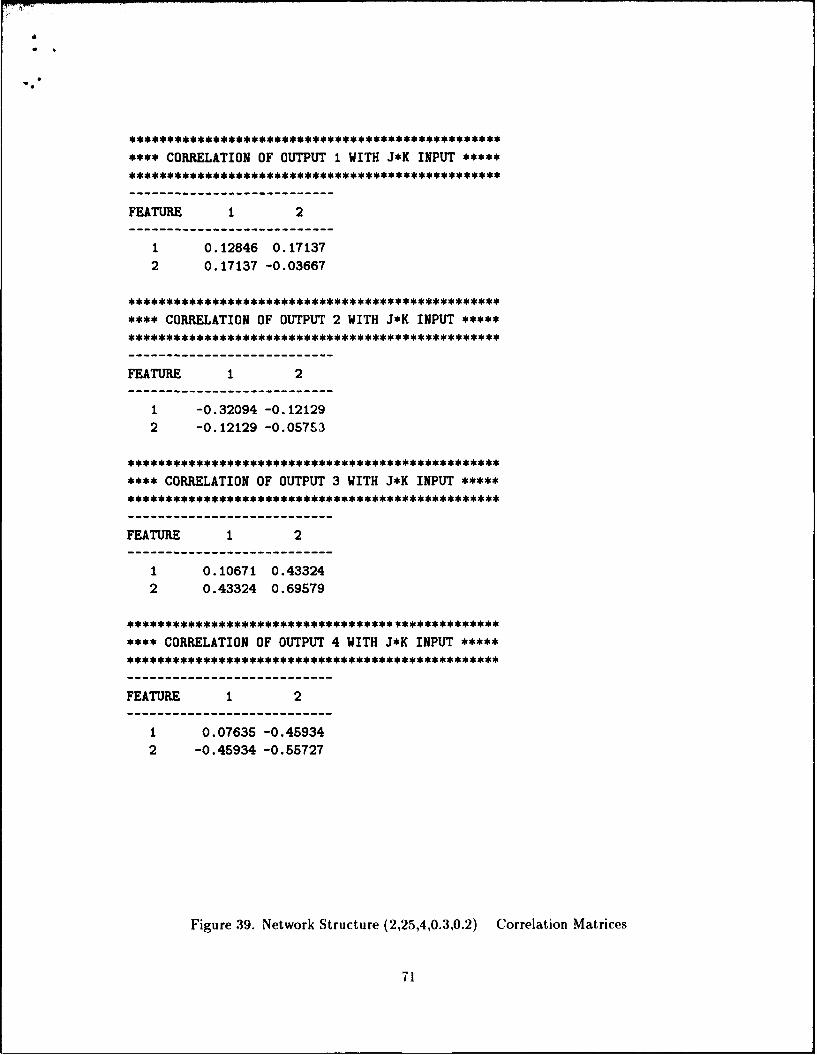
2.6 High-Order Inputs and Correlation
Networks that have second, third or greater order terms for inputs are referred to as
high-order networks. If two inputs x, and x2 represent two separate pieces of information,
then x2 or xIx 2 may represent pieces of information more important to discrimination than
either one separately. Giles suggests that an examination of correlation matrices which
relate the high-order input terms with the outputs of a trained network would be useful.
The entries in the correlation matrix that have the largest absolute value correspond to the
high-order input terms that should be considered for inclusion in the network [6:4977-4978].
We will use the following equations to calculate the second-order correlation matrix of the
product of two inputs with the output. These equations and notation were developed by
Belue and Bauer [2:9].
First, define the sample covariance C(i, (j, k)), between the ith output node of the
network and the second-order product of the jth and kth input nodes as:
and x8(j) is the value of the jth feature in exemplar s, x-(k) is the value of the kth feature
in exemplar s, zr(s) is the output of output node i for exemplar s and N is the number of
exemplars in the training set.
Next, define an element of the second-order correlation matrix R(i, (j, k)), as the
correlation between the ith output node of the network and the second-order product of
the jth and kth input nodes where:
23
R(i,(j,k)) = C Uij k))
1 [zr(s) - T(i)I2f [z, - (j, k)]2 (26)
The entries in the correlation matrix that are greatest in absolute value correspond to
second-order terms that are highly correlated with output i.
2.7 The Shell-Mezgar Sort
Empirical evidence has shown that a reshuffling of training vectors at the beginning of
each epoch will yield superior results [20:99-100]. With some networks requiring thousands
of epochs before they are trained, it is wise to incorporate an efficient reshwlif*ing algorithm
into the software. By generating a random number for each training vector and then
sorting on these random numbers, we can reshuffle the training vectors. Therefore, the
efficient reshuffling algorithm that we seek transforms into an efficient sort algorithm.
According to Press, et.al., for the basic task of sorting N elements, the best sort
algorithms require on the order of several times N1og 2N operations. The algorithm inventor
tries to reduce the constant in front of this estimate to as small a value as possible [13:226-
229]. Knuth has shown that for "randomly" ordered data, the operations count on the
Shell-Mezgar sort goes approximately as N 12 , for N < 60000 [9]. Since our sort index
consists of random numbers, and the number of training vectors will be < 60000, the
Shell-Mezgar sort is an ideal candidate. In chapter 4 there is a table which compares
Nlog2N and N1. 27 for various values of N. A FORTRAN version of this sorting routine
may be found in Press, et.al. [13:226-229].
24
IHL Methodology
The overall objective of this thesis was to develop software to assist the researcher
in building an appropriate back-propagation neural network. The software was to enable
the researcher to quickly define a neural net structure, run the neural network, interrupt
training at any point to analyze the status of the current network, re-start training at the
interrupted point if desired, and analyze the final network. What follows is a synopsis of
each of the subroutines found in the FORTRAN code as well as the MATLAB interface.
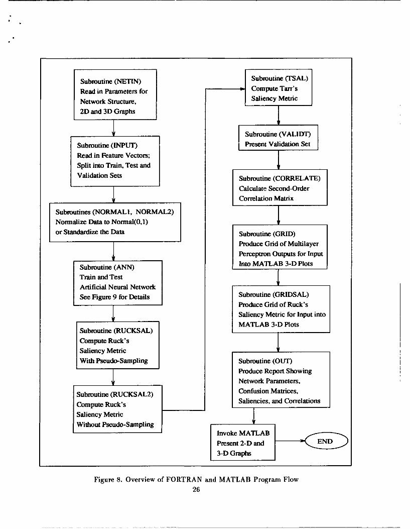
By following the program flow we can define the methodology used. Figure 8 shows the
overall program flow.
3.1 Defining Neural Network Parameters
The subroutine NETIN reads all network parameters from a user designated param-
eter file. These parameters name the raw data file, determine a stopping criteria, layout
the neural network structure, and define the desired 2D and 3D graphs. An explanation
of the required parameters follows. The FORTRAN program will prompt the user for the
name of this parameter file. Appendix A gives an example of such a parameter file and
defines the allowable values.
"* Data File Name This parameter defines the name of the data set where all the raw
data resides. Training, test, and validation sets will be pulled from this data set in
a random order.
"* Stopping Criteria Determines when training of the neural network will end. The
user can specify number of epochs or average absolute error as the stopping criteria.
If number of epochs is specified, the program will stop and present the network
results as they existed at the end of the specified epoch. If average absolute error is
specified, the program will stop when the average absolute error (for the training or
test set) at the end of an epoch is less than or equal to the specified error rate. It
should be noted that this parameter is over-ridden if the user terminates training of
the network interactively. See sub-section 3.4.3.
25
Subroutine (NETIN) Subroutine (TSAL)
Read in Parameters for Compute Tafr's
Network Structure, Saliency Metric
2D and 3D Graphs F
I _ Subroutine (VALIDT)
Subroutine (INPUT) Present Validation Set
Read in Feature Vectors;
Split into Train, Test and
Validation Sets Subroutine (CORRELATE)
Calculate Second-Order
Correlation Matrix
Subroutines (NORMALI, NORMAL2)
Normalize Data to Normal(0,l)
or Standardize the Data Subroutine (GRID)
Produce Grid of Multilayer
Perceptron Outputs for Input
Subroutine (ANN) Into MATLAB 3-D Plots
Train and Test
Artificial Neural Network
See Figure 9 for Details Subroutine (GRIDSAL)
Produce Grid of Ruck's
Saliency Metric for Input into
MATLAB 3-D PlotsSubroutine (RUCKSAL)
Compute Ruck's
Saliency Metric
With Pseudo-Sampling Subroutine (OUT)
Produce Report Showing
Network Parameters,
Subroutine (RUCKSAL2) Confusion Matrices,
Compute Ruck's Saliencies, and Correlations
Saliency Metric
Without Pseudo-SamplingInvoke MATLAB
Present 2-D and
3-D Graphs
Figure 8. Overview of FORTRAN and MATLAB Program Flow
26
"* Number of Training Vectors (NI) Defines the number of vectors to be put into
the training set.
"* Number of Test Vectors (N2) Defines the number of vectors to be put into the
test set.
"* Number of Validation Vectors (N3) Defines the number of vectors to be put into
the validation set.
"* Number of Input Nodes This parameter is equal to the number of features or
independent variables found in each vector.
"* Number of Middle Nodes The user must determine the number of middle nodes
required in the network structure. This may have to be determined through experi-
mentation.
"* Number of Output Nodes This parameter is equal to the number of output classes
found in each vector.
"* Type of Learning Rate (LTYPE) Defines the type of learning rate that will be used
in the back-propagation algorithm. There are six types of learning rates: constant,
linear, log, log-linear, loq-square root, and log-square root linear. See Appendix A
for a detailed description of the learning rates supported by this software.
"* Learning Rate Gives the constant learning rate value, if (LTYPE=1) in the pa-
rameter above. If (LTYPE $ 1), this parameter is ignored.
"* Momentum Rate Defines the constant momentum rate that will be used in the
back-propagation algorithm. If no momentum rate is desired, set momentum rate
equal to zero.
"* Range of Weight Initialization Before beginning the back-propagation algorithm,
the program must initialize all weights between the nodes to random numbers. The
random number generator used in the FORTRAN program generates Uniform(O, 1)
random deviates U. These random deviates are then run through a transformation
function of the form:
a + (b - a)U (27)
27
where a is the desired lower limit of the range initialization, and b is the desired
upper limit. In effect, we are generating random deviates with a Uniform(a,b)
distribution.
"* Random Number Seed Defines the seed for the random number generator used
in initializing weights and determining the sort order of the training set.
"* Type of Normalization of Data Determines if data is to be normalized. User may
normalize data between (0, 1), standardize the data, or use the data in its original
form.
"* Number of Divisions for Pseudo-sampling This parameter is used when calcu-
lating Ruck's saliency. This is the value of R as described in Equation 22.
"* Graphics Parameters Define 2D and 3D graphs which will be created by MAT-
LAB. See Appendix A for details.
3.2 Defining Train, Test and Validation Sets
The subroutine INPUT reads the raw data from a single file. Each input line is an
exemplar or case. This case vector consists of feature values and the corresponding correct
classification. For example, a problem with two input features x, and x2, and four output
classes c1 ,c 2 , c 3 and c4 , would have the following input vector: (xI,x 2,c 1 ,c 2,c 3 ,c 4 ). If a
particular case had a correct classification of class 3 the vector would be: (x 1, x 2, 0, 0, 1,0)
A random number is generated and attached to each vector. We then perform a Shell-
Mezgar sort on the vectors using these random numbers as the sort index. We then place
the first N1 vectors in the training set, the next N2 vectors in the test set, and finally the
last N3 vectors in the validation set, wher N1, N2 and N3 are defined in the parameter
file described above. This procedure randomly creates the training, test and validation
sets. To create different sets, simply change the random number seed in the parameter file.
These three sets of vectors will remain fixed throughout the entire computer run. However,
the vectors within the training set are reshuffled after each epoch.
28
3.3 Normalization of Data
The subroutines NORMAL1 and NORMAL2 normalize the data now residing in the
train, test and validation sets. The user has the option, as specified in the parameter file,
of not normalizing the data at all, normalizing between 0 and 1, or performing Gaussian
normalization. Subroutine NORMAL1 normalizes each of the feature vectors to values
between 0 and 1, based on the range of the training set. The test set and validation set
are also normalized based on the range of the training set. By basing normalization on
the training set only, we keep everything on the same scale.
Subroutine NORMAL2 statistically normalizes each of the feature vectors to values
based on the mean and standard error of the training set. Let xi be the vector value of
the ith feature, ii be the mean of feature i over the training set and si be the standard
deviation. Then for every vector in the training, test and validation set, the normalized
ith feature is:
X1 = (28)Ssi
This procedure is known as standardization. Ruck refers to it as Gaussian Normalization
[16:15-16].
3.4 Artificial Neural Network (ANN)
Subroutine ANN is the heart of this FORTRAN based neural network system. It
is where the back-propagation algorithm is performed. Figure 9 gives a detailed flow
of the subroutine ANN. This subroutine assumes the following network structure and
characteristics:
"* Fully connected feed-forward perceptrons
"* Back-propagation training as defined in Equations 18 and 19.
"* Single hidden layer
"* Sigmoid non-linear transformation
The artificial neural net subroutine begins by initializing the weights connecting both
the input layer and hidden layer and the hidden layer and output layer. Normally, these
29
Randomize Weights
Calculate Learning Begin Another Epoch
Rate and Reshuffle
Training Vectors
Present a TrainingExemplar
if No
Calculate Actual
Output Program No Acceptable
SInterrupted Error Rate or
By User ? Final Epoch ?
SYes Yes
Call MATLABPresent
Compare Network vs 2-D Graphs
Desired Outputs and
UPDATE WEIGHTSS~User Terminates
Training? NoAll Training
N Vectors Presented ? FI1
YeseI Yes STOP TRAINING L
Present TestData Data END Subroutine
ANN
Figure 9. Subroutine ANN Program Flow30
weights are random numbers between -.5 and +.5. This range of weight initialization is
controlled by the user from the input parameter file. After the random initialization is
complete, the program begins epoch number one. Each presentation of the set of training
vectors and test vectors is defined as an "epoch".
3.4.1 Calculations By Epoch. At the beginning of each epoch a learning rate
is calculated. Except for the constant learning rate, all learning rates are a function of
the specific epoch number. As the epoch number increases, all learning rate functions are
designed to decrease. Recall that the selection of a learning rate is of critical importance
in finding the true global minimum of the absolute error. Back-propagation training with
too small a learning rate is agonizingly slow, but too large a learning rate may produce
oscillations between relatively poor solutions. See Appendix A, for specific learning rate
functions.
The next step in the ANN subroutine is the reordering of the feature vectors in the
training set into a random list. Random ordering prevents the network from learning the
order of the data and may speed the training time. This random reordering is accomplished
by attaching a random number to each training vector and then using the random number
as a sort key. A Shell-Mezgar sort is then applied to the set of training vectors. As
mentioned in Section 2.7, this sort needs to be very efficient since it is performed at the
beginning of each epoch, which may number in the thousands.
With the training set randomly sorted, we are ready to begin training of the weights
in the network. For each exemplar in the training set the algorithm performs the following
three steps. First an activation of the hidden layer and output layers is calculated using
the sigmoid non-linear transformation. Second, the activations of the output layer are
compared to the desired (known) output and placed into the training set confusion ma-
trix. Finally, the back-propagation training procedure is performed updating the network
weights. After all the training vectors have been presented to the network, the weights
are held constant and the test vectors are presented to the perceptron. Once again, the
activations of the output layer are compared to the desired (known) output, but this time
placed into the test set confusion matrix. After all training and test vectors have been
31
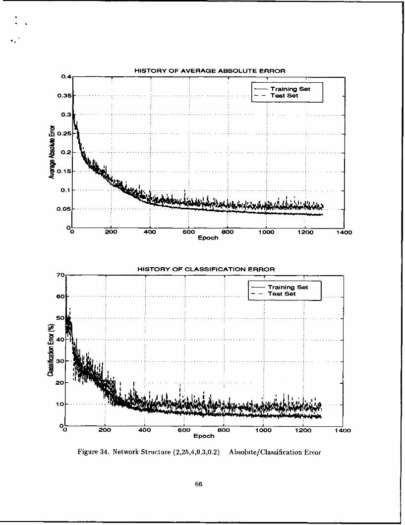
presented to the network, an average absolute error and classification error are calculated
for the training and test sets. These two errors appear on the 2D graphs produced by
MATLAB. They are used as an indicator of the performance of the network. By collecting
the absolute error and classification error for the two sets at the end of each epoch, an
error curve can be constructed and a minimum error observed somewhere along this curve.
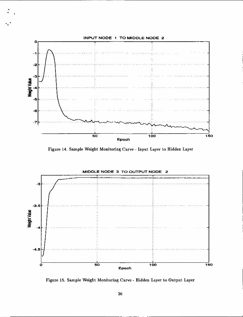
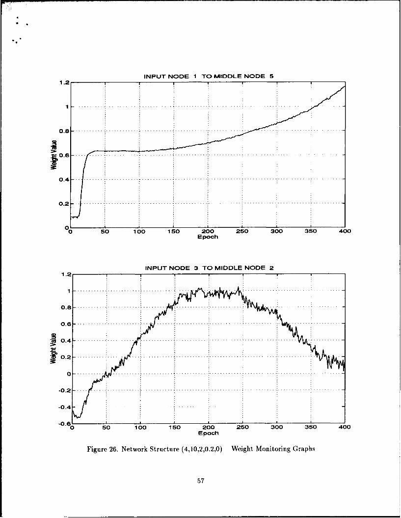
In addition, the weights specified by the user to be monitored are saved at the end of each
epoch. By graphing these weights, we can see how they have changed over the entire run.
Some will be trained and remain relatively constant, while others will still be increasing
or decreasing.
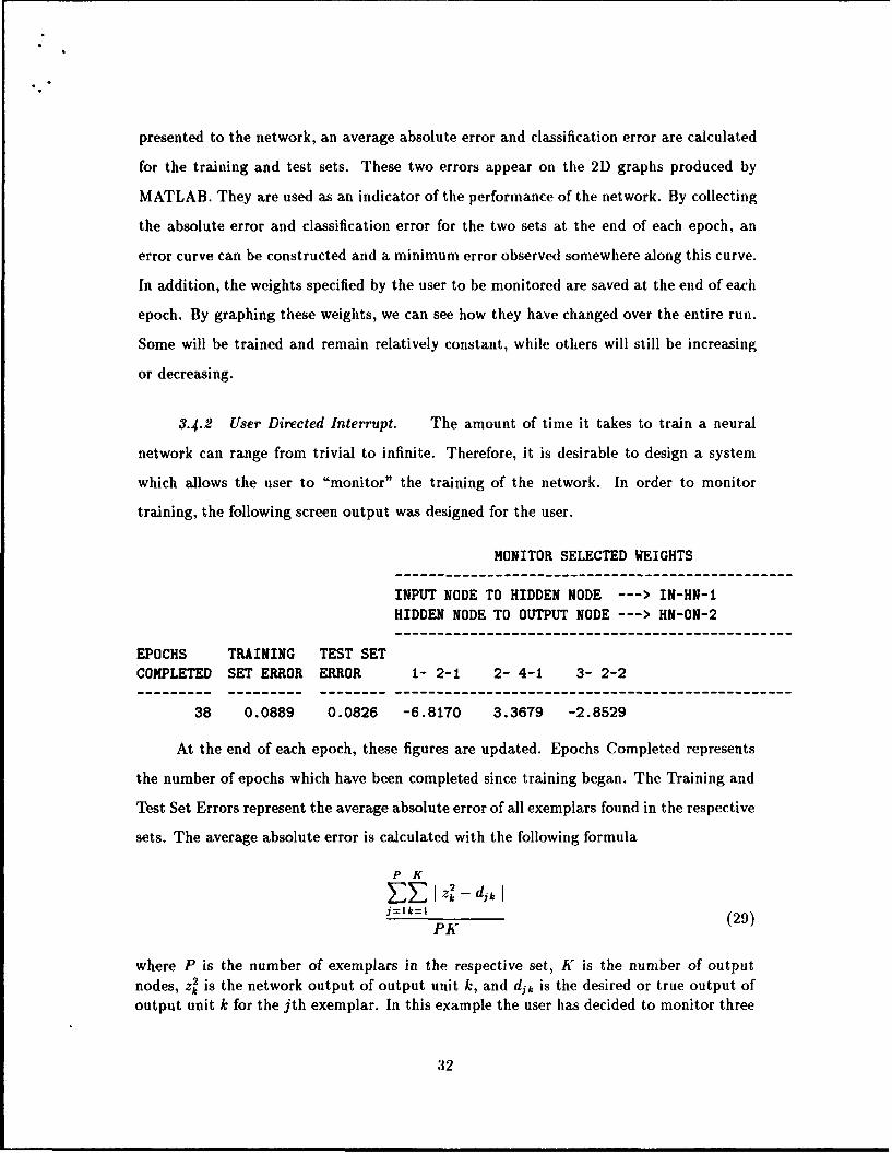
3.4.2 User Directed Interrupt. The amount of time it takes to train a neural
network can range from trivial to infinite. Therefore, it is desirable to design a system
which allows the user to "monitor" the training of the network. In order to monitor
training, the following screen output was designed for the user.
MONITOR SELECTED WEIGHTS
INPUT NODE TO HIDDEN NODE --- > IN-HN-1HIDDEN NODE TO OUTPUT NODE --- > HN-ON-2
EPOCHS TRAINING TEST SETCOMPLETED SET ERROR ERROR 1- 2-1 2- 4-1 3- 2-2
38 0.0889 0.0826 -6.8170 3.3679 -2.8529
At the end of each epoch, these figures are updated. Epochs Completed represents
the number of epochs which have been completed since training began. The Training and
Test Set Errors represent the average absolute error of all exemplars found in the respective
sets. The average absolute error is calculated with the following formula
P K
j=Ik=1 (29)PK
where P is the number of exemplars in the respective set, K is the number of outputnodes, z4 is the network output of output unit k, and dik is the desired or true output ofoutput unit k for the jth exemplar. In this example the user has decided to monitor three
32
different weights. For example, the second monitored weight is designated "2-4-1". Thecode "2-4-1" indicates the user is monitoring the weight connecting input node 2 to hiddennode 4 of layer 1. The third monitored weight is designated "3-2-2". The code "3-2-2"indicates the user is monitoring the weight connecting hidden node 3 to output node 2 oflayer 2. To help the researcher keep these indices straight, the heading provides a simplekey:
INPUT NODE TO HIDDEN NODE --- > IN-HN-1HIDDEN NODE TO OUTPUT NODE --- > HN-ON-2
where IN represents the input node, HN the hidden node, and ON the output node.
The last digit represents the layer.
As the user watches the epochs "tick" by (or comes back to the terminal after lunch
or the following day for a "large" neural net), they can interrupt the training procedure at
any time. See Appendix A for details. At the end of each epoch subroutine ANN checks
to see if the user has interrupted training of the network. If it detects an interrupt the
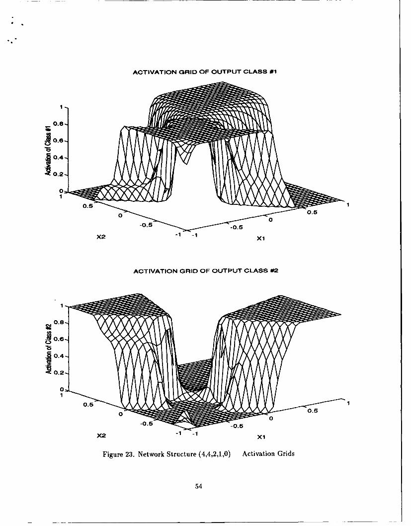
FORTRAN program pauses, creates an input file for MATLAB called "plotdatl.m", and
calls MATLAB. The MATLAB program automatically produces four separate graphs of
error curves. See Figures 10, 11, 12, and 13. Figure 10 shows the average absolute error of
the training and test sets for each epoch, while Figure 11 displays the same information for
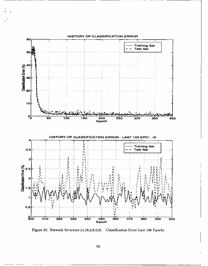
the last 100 epochs only. Figure 12 shows the classification errors of the training and test
sets for each epoch, while Figure 13 displays the same information for the last 100 epochs
only. In addition to the four graphs mentioned above, the user has designated specific
weights to monitor in the parameter file. A graph is produced for each weight specified.
See Figures 14, and 15.
The goal is to cease training at the point corresponding to a minimum error on the test
set. The choice of this point may be difficult since it is necessary to consider both average
absolute error and classification error. After analyzing the graphs the researcher must
determine if additional training of the network is required, or if the network is sufficiently
trained. After quitting the MATLAB program, the FORTRAN program prompts the
user for their decision. If its determined that additional network training is required, the
program will begin at the point where it was interrupted. No information from prior
training is lost. The user may interrupt the training process as often as necessary. If its
determined that the network is sufficiently trained, the program saves all information as
33
HISTORY OF AVERAGE ABSOLUTE ERROR0.6
Training Set-- Test Set
LUJ
_0 50o 100 150Epoch
Figure 10. Sample Average Error Distance Curves for Training and Test Sets
HISTORY OF AVG ABSOLUTE ERROR - LAST 100 EPOCHS0.09
I~ Taining Set0.08 - -Test Set
e'If ll I % i
-2 0 .0 8 ..... ... . .. ... .... ... .. .. .
~0.0 5 .. .. . .1 ... .. .. ..
a s ... .. II I I 1 1 : j . ; 1 ;J
~0.06 - ... .... I !..
S it
0.055 -' ....
0.05
004o 6 70 80 90 100 110 120 130 140 150Epoch
Figure 11. Sample Average Error Distance Curves -Last 100 Epochs Only
ICLASS lICLASS 21 TOTAL I-----------------4-----------4------------
I ICLASS 11 99 I 8 I 10711 T 1 I 92.52%1 7.48%1 I1 R I ------------------------------------I U ICLASS 21 15 I 103 I 11811 E 1 I 12.71%1 87.29%1 I1 I ----------------------------I I TOTAL I 1141 1111 2251
I ICLASS 11 106 I 1 I 10711 T 1 I 99.07%I 0.93%1 I1 R I ------------------------------------I U ICLASS 21 0 I 118 I 11811 E I 1 0.00oI 100.001 II I ---------------- +-----------+------------
ICLASS lICLASS 21 TOTAL I-------------------------------------------
ICLASS 11 67 1 0 I 6711 T I I 100.00ol 0.00%1 IIR I ÷------------------------ ------------I U ICLASS 21 1 I 57 I 581I E I I 1.72%1 98.28%1 I1 I --- ------------- +-----------+------------
ICLASS lICLASS 21CLASS 31CLASS 41 TOTAL I----------- +-----------4-----------4------------+-----------+------------
I ICLASS 11 193 I 9 I 3 I 2 I 20711 T 1 I 93.24%1 4.35%1 1.45%l 0.97%1 I1 R I --------------------------------- +------- +------------I U ICLASS 21 10 I 201 I 1 I 1 I 21311 E 1 I 4.69%1 94.37Xl 0.47%1 0.47%1 I1-------+---------+-----------4------------+-----------4------------
ICLASS 31 6 I 1 I 174 I 0 I 18111 1 I 3.31%1 0.55X1 96.13%1 0.00%1 II I------------+-----------+-----------+-----------4------------I ICLASS 41 1 I 1 1 0 I 197 I 19911 1 I 0.50I1 0.50l 0.oo00 98.99%l I
1 I -------- +-----------+-----------+-----------+-----------
I I TOTAL I 2101 2121 1781 2001 8001
Figure 35. Network Structure (2,25,4,0.3,0.2) Confusion Matrix for Training Set
ICLASS lJCLASS 21CLASS 31CLASS 41 TOTAL I---------------+-----------+-----------+-----------+------------
I ICLASS 11 32 I 7 I " 0 I 1 I 4011 T 1 1 80.00%1 17.50%1 0.00%1 2.50%1 1
1R I -------------------------------------------------------I U ICLASS 21 0 1 so 1 0 1 01 501I E I 1 0.00o1 100.00o1 0.00o 1 0.00o1 II I---------------+-----------+-----------+-----------+------------I ICLASS 31 0 I 0 I 29 1 1 I 3011 1 I 0.00%1 0.00%1 96.67%1 3.33%1 I
1 TYPE OF LEARNING RATE (e.g. 1-Constant, 4-Log-Linear, etc...)
0.2 LEARNING RATE (Only used when TYPE OF LEARNING RATE - 1 or 2)
0.0 MOMENTUM RATE
-0.5 0.5 RANGE of Weight Initialization
1234567 SEED for Random Number Generator
1 Type of NORMALIZATION of data.
5 Number of Divisions for Pseudo-Sampling for RUCK'S SALIENCY
999 Constant for GRID and GRID Saliency Plots. 999 -- > Use Feature Average
2 Number of WEIGHTS TO MONITOR During Training
4 1 1 FROM Node/TO Node/LAYER
922
2 Number of ACTIVATION GRIDS to Plot
3 4 1 * of FEATURE for X-AXIS / S of FEATURE foi Y-AXIS / Activation Class
Mass
Secant
1 4 1 * of FEATURE for X-AXIS / * of FEATURE for Y-AXIS
Ply
Secant
2 Number of SALIENCY GRIDS to Plot
3 4 3 * of FEAT for X-AXIS/* of FEAT fr Y-AXIS/S OF FEAT for SALIENCY
Mass
Secant
Mass
3 4 4 * of FEAT for X-AXIS/S of FEAT for Y-AXIS/S OF FEAT for SALIENCY
Mass
Secant
Secant
END
86
Bibliography
1. Belue, Capt Lisa M. An Investigation of Multilayer Perceptrons for Classification.MS thesis, AFIT/GOR/ENS/92M-06. School of Engineering, Air Force Institute ofTechnology (AU), Wright-Patterson AFB OH, March 1992.
2. Belue, Lisa M. and Kenneth W. Bauer Methods of Determining Input Features forMultilayer Perceptrons. Working Paper. School of Engineering, Air Force Institute ofTechnology (AU), Wright-Patterson AFB OH, September 1993.
3. Cybenko G. "Approximations by Superpositions of Sigmoidal Functions," Mathemat-ics of Controls, Signals, and Systems (1989). Accepted for publication.
4. Defense Advanced Research Projects Agency (DARPA). Neural Network StudyAFCEA International Press, Fairfax VI, November 1988.
5. Foley, Donald H. "Considerations of Sample and Feature Size," IEEE Transactionson Information Theory, 18: 618-626 (September 1972).
6. Giles, Lee C. and Tom Maxwell. "Learning Invariance, and Generalization in High-order Neural Networks," Applied Optics, 26: 4972-4978 (1 December 1987).
7. Hecht-Nielsen, Robert. Neurocomputing. New York: Addison-Wesley, 1990.
8. Hornik, K., M. Stinchcombe, and H. White. "Multilayer Feedforward Networks AreUniversal Approximators," Neural Networks, 2: 359-366 (May 1989).
9. Knuth, Donald E. "Sorting and Searching," The Art of Computer Programming, 3:Reading, MA: Addison-Wesley, 1973.
10. Lippmann, Richard P. "An Introduction to Computing with Neural Nets," IEEEAcoustics, Speech, and Signal Processing. 4-22 (April 1987).
11. McClelland, J., and Rumelhart, D. Explorations in Parallel Distributed Processing.Cambridge, MA: The MIT Press, 1988.
12. Minsky, Marvin Lee and Seymour Papert. Perceptrons (Expanded Edition). Cam-bridge, MA: The MIT Press, 1988.
13. Press, William H., Brian P. Flannery, Saul A. Teukolsky, and William T. Vettering.Numerical Recipes [FORTRAN Version]. Cambridge University Press, 1989.
14. Rogers, Maj Steven K., Matthew Kabrisky, Dennis W. Ruck, and Gregory L. Tarr.An Introduction to Biological and Artificial Neural Networks. Unpublished Report.School of Engineering, Air Force Institute of Technology (AU), Wright-Patterson AirForce Base, OH, October 1990.
15. Rosenblatt, R. Principles of Neurodynamics. New York, Spartan Books, 1959.
16. Ruck, Capt Dennis W. Characterization of Multilayer Perceptrons and Their Applica-tion to Multisensor Automatic Target Detection. PhD dissertation. School of Engineer-ing, Air Force Institute of Technology (AU), Wright- Patterson AFB OH, December1990 (AD-A229035).
17. Ruck, Capt Dennis W. "Feature Selection Using a Multilayer Perceptron," Journal ofNeural Network Computing, 20: 40-48 (Fall 1990).
87
18. Steppe, Capt Jean M. Feature Selection in Feedforward Neural Networks PhD dis-sertation prospectus. School of Engineering, Air Force Institute of Technology (AU),Wright-Patterson AFB OH, October 1992.
19. Tarr, Capt Gregory L. Multi-layered Feedforward Neural Networks for Image Segmen-tation. PhD dissertation. School of Engineering, Air Force Institute of Technology(AU), Wright-Patterson AFB OH, November 1991.
20. Weiss, Sholom M. and Casimir A. Kulikowski. Computer Systems That Learn. MorganKaufmann Publishers, Inc., 1991.
88
Vita
Captain Gregory L. Reinhart was born on 27 September 1955 in Buffalo, Minnesota.
In 1973, he graduated from Loyola High School of Mankato Minnesota. In 1977, he gradu-
ated magna cum laude from Mankato State University with a Bachelor of Science Degree
in Mathematics. A Distinguished Graduate from Undergraduate Navigator Training, his
first assignment was as a C-141 navigator at Norton AFB, California, where he earned his
qualification as a Special Operations Low Level instructor navigator. A subsequent assign-
ment took him to 21st Air Force, AMC, McGuire AFB, New Jersey, where he supported
the flight planning and diplomatic clearance section and became assistant chief of the Spe-
cial Operations Division. Captain Reinhart entered the Air Force Institute of Technology
I AGENCY' ME O1CY V H &2RP~ A ~ 3 PORT TYPI AN DATI
_) March 1994 Master's Thesisý4. ThiLt AANL Suh'7tE N ~ ,
A FORTRAN BASED LEARNING SYSTEM USING MULTILAYERBACK-PROPAGATION NEURAL NETWORK TECHNIQUES
Gregory L. Reinhart, Capt, USAF
Air Force Institute of Technology, WPAFB OH 45433-6583 AFIT/GOR/ENS/94M-11
N/A
Approved for public release; distribution unlimited
An interactive computer system which allows the researcher to build an "optimal" neural network structurequickly, is developed and validated. This system assumes a single hidden layer perceptron structure and usesthe back-propagation training technique. The software enables the researcher to quickly define a neural networkstructure, train the neural network, interrupt training at any point to analyze the status of the current net-work, re-start training at the interrupted point if desired, and analyze the final network using two-dimensionalgraphs, three-dimensional graphs, confusion matrices and saliency metrics. A technique for training, testing, andvalidating various network structures and parameters, using the interactive computer system, is demonstrated.Outputs automatically produced by the system are analyzed in an iterative fashion, resulting in an "optimal"neural network structure tailored for the specific problem. To validate the system, the technique is applied totwo, classic, classification problems. The first is the two-class XOR problem. The second is the four-class MESHproblem. Noise variables are introduced to determine if weight monitoring graphs, saliency metrics and saliencygrids can detect them. Three dimensional class activation grids and saliency grids are analyzed to determineclass borders of the two problems. Results of the validation process showed that this interactive computer systemis a valuable tool in determining an optimal network structure, given a specific problem.


![KOSELLECK, REINHART - Aceleración, Prognosis y Secularización [Por Ganz1912]](https://static.documents.pub/doc/80x56/5695d0141a28ab9b0290dead/koselleck-reinhart-aceleracion-prognosis-y-secularizacion-por-ganz1912.jpg)


