D. McCallenYucca Mountain and Repository Science

ProgramLawrence Livermore National Laboratory

Livermore, California

Evaluating Fragile Blades and Filaments in the Lithophysae for Constraints on Long Return Period

Earthquake Ground Motions at Yucca Mountain Nevada

August 2004 Workshop on Extreme Ground Motions at Yucca Mountain

USGS, Menlo Park Ca

Evaluating Fragile Blades and Filaments in the Lithophysae for Constraints on Long Return Period

Earthquake Ground Motions at Yucca Mountain Nevada

August 2004 Workshop on Extreme Ground Motions at Yucca Mountain

USGS, Menlo Park Ca

J. WhelanEnvironmental Science Team

Yucca Mountain Project BranchUnited States Geological Survey

Denver, Colorado

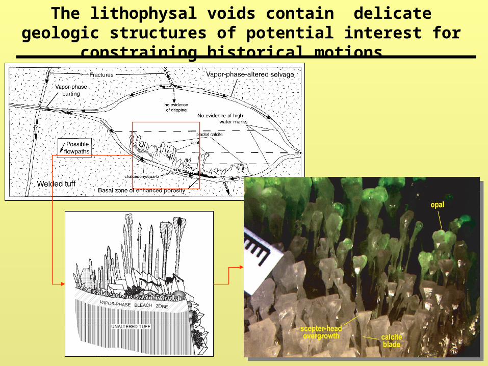
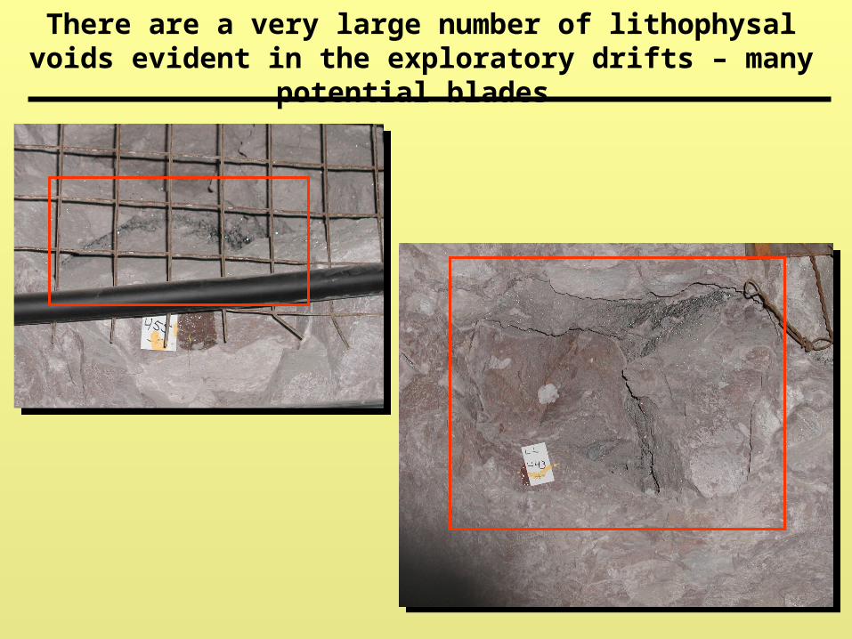
The lithophysal voids contain delicate geologic structures of potential interest for constraining

historical motions

Tpt

Tcp

Tcp

GDF

Tcp

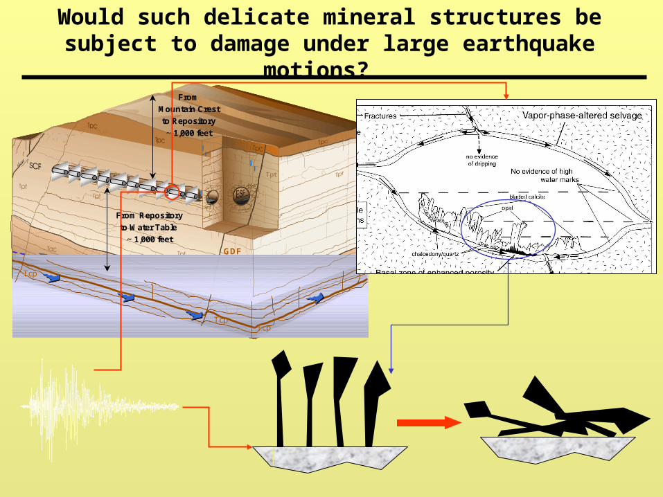
From

Mountain Crest

to Repository

~ 1,000 feet

From Repository

to Water Table

~ 1,000 feet

Tpt

Tcp

Tcp

GDF

Tcp

From

Mountain Crest

to Repository

~ 1,000 feet

From Repository

to Water Table

~ 1,000 feet

Would such delicate mineral structures be subject to damage under large earthquake motions?

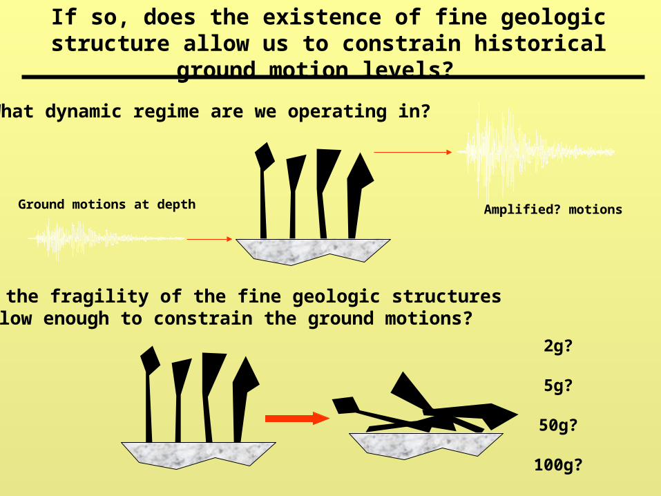
If so, does the existence of fine geologic structure

allow us to constrain historical ground motion levels?

• What dynamic regime are we operating in?

• Is the fragility of the fine geologic structures low enough to constrain the ground motions?

2g?

5g?

50g?

100g?

Ground motions at depth Amplified? motions

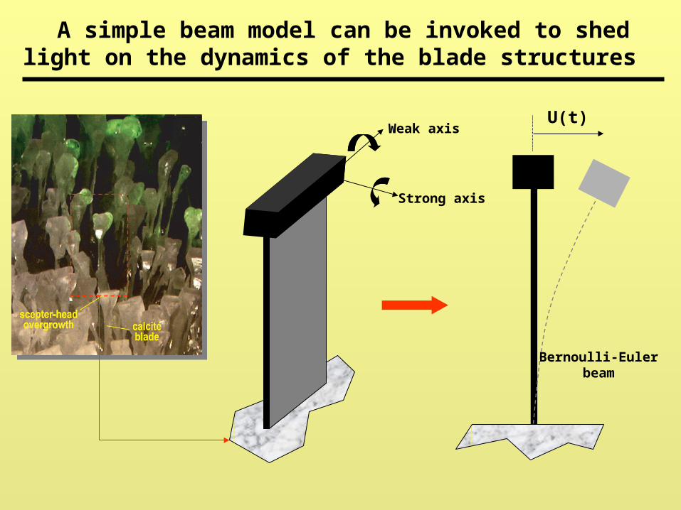
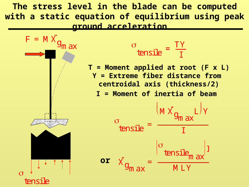
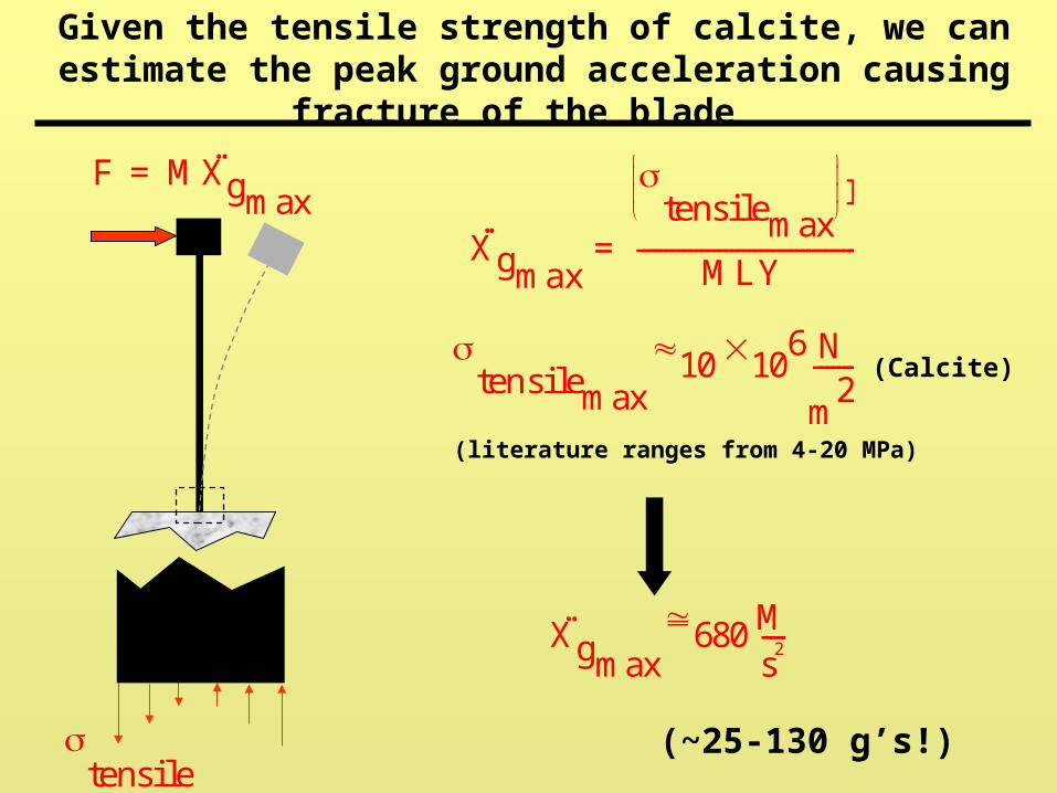
A simple beam model can be invoked to shed light on the dynamics of the blade structures

Weak axis

Strong axis

U(t)

Bernoulli-Eulerbeam

KK

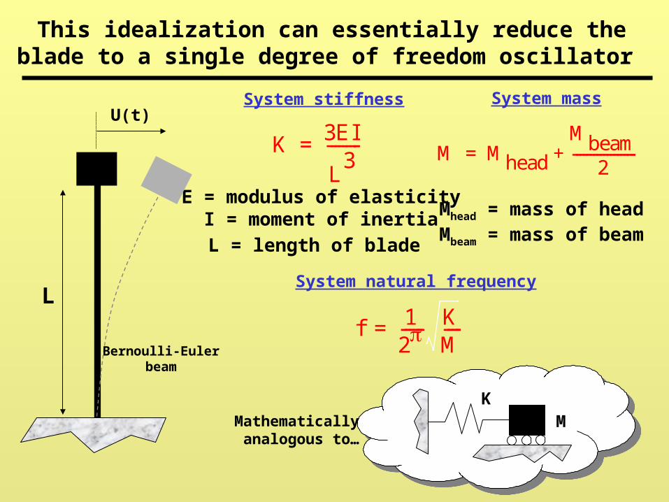
This idealization can essentially reduce the blade to a single degree of freedom oscillator

System stiffness

E = modulus of elasticityI = moment of inertia

L = length of blade

U(t)

Bernoulli-Eulerbeam

L

System mass

System natural frequency

M Mhead

Mbeam2

-------------------+=

f 12------ K

M-----=

Mhead = mass of headMbeam = mass of beam

M

K 3EI

L3

---------=

Mathematically analogous to…

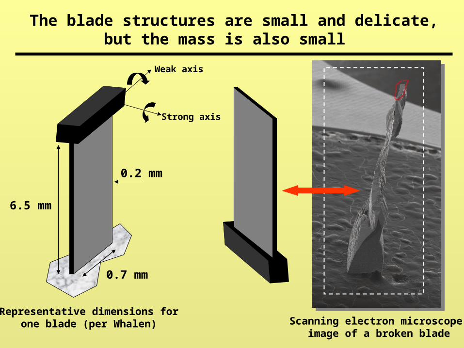
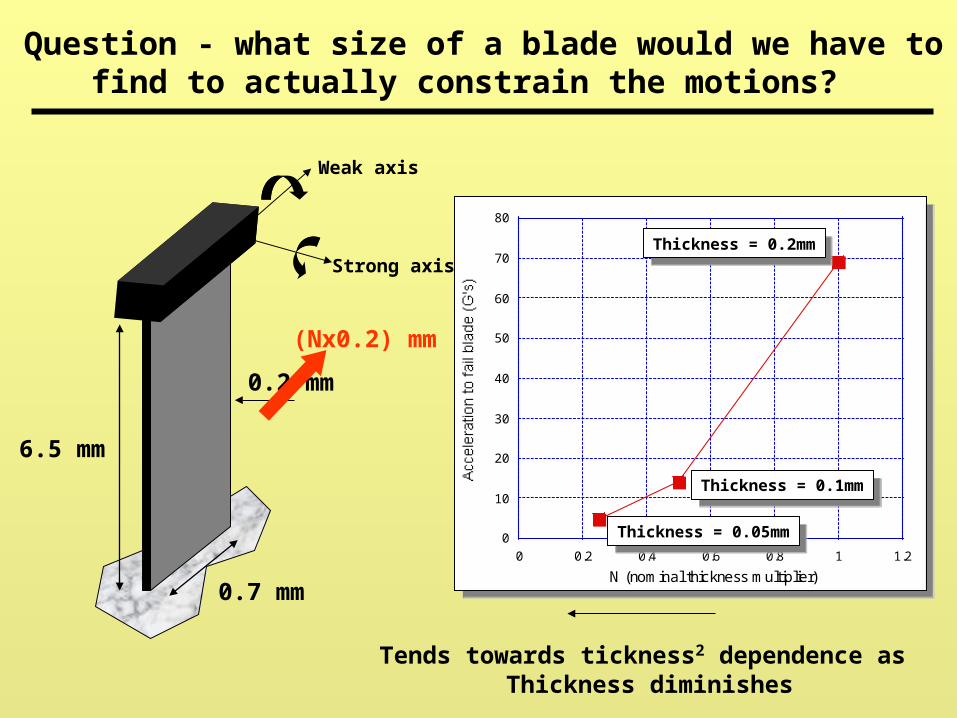
The blade structures are small and delicate, but the mass is also small

Weak axis

Strong axis

6.5 mm

0.7 mm

0.2 mm

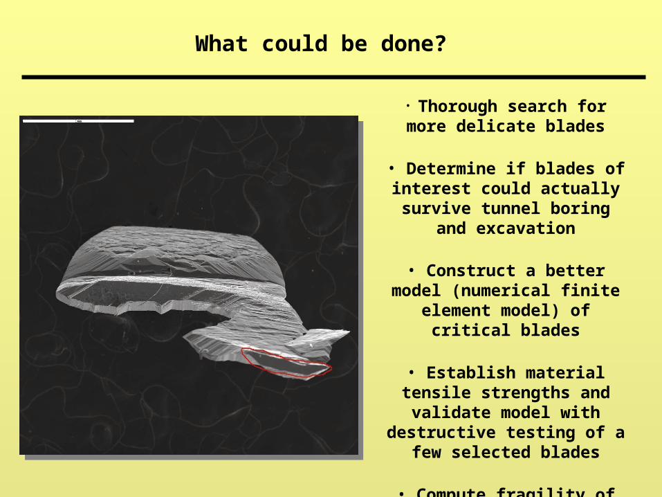
Scanning electron microscope image of a broken blade

Representative dimensions forone blade (per Whalen)

The frequency of the current blade identified in the USGS inventory is quite high

Stiffness

Value (K)428 (N/m)

E = 8.4 x 1010 N/m2

I = 4.667 x 10-16 m4

L = 6.5 x 10-3 m

Mass

Value (M)1.042 x 10-5 (Kg)

½ Beam mass =

1.229 x 10-6 Kg

Opal head mass =

9.196 x 10-6 Kg

Frequency

(Hz)~1000 (Hz)

Mother Nature is

not cooperating!

The frequency of the blade is quite high compared to the dominant frequencies of the YMP

motions

-20

-15

-10

-5

0

5

10

15

0 50 100 150

mat01h11

Time (sec)

-20

-15

-10

-5

0

5

10

15

0 50 100 150

mat01h11

Time (sec)

0

20

40

60

80

100

0 2 4 6 8 10

mat01h11

Period (Sec)

0

20

40

60

80

100

0 2 4 6 8 10

mat01h11

Period (Sec)

1000 Hz = 0.001 sec

Due to the high frequency of the blade, it will respond essentially as a rigid body to the

earthquake motions

F MX··gmax=

-20

-15

-10

-5

0

5

10

15

0 50 100 150

mat01h11

Time (sec)

-20

-15

-10

-5

0

5

10

15

0 50 100 150

mat01h11

Time (sec)

X··gmax

Bendingstresses

The stress level in the blade can be computed with a static equation of equilibrium using peak ground

acceleration F MX··gmax

=

tensile

T = Moment applied at root (F x L)Y = Extreme fiber distance from

centroidal axis (thickness/2)

I = Moment of inertia of beam

tensile

TYI

--------=

tensile

MX··gmaxL

Y

I--------------------------------------=

X··gmax

tensilemax

I

MLY--------------------------------------=or

Given the tensile strength of calcite, we can estimate the peak ground acceleration causing

fracture of the blade

F MX··gmax=

tensile

X··gmax

tensilemax

I

MLY--------------------------------------=

(Calcite)

(~25-130 g’s!)

X··gmax680 M

s2-----

tensilemax

10 106 N

m2

-------

(literature ranges from 4-20 MPa)

Question - what size of a blade would we have to find to actually constrain the motions?

Weak axis

Strong axis

6.5 mm

0.7 mm

0.2 mm

(Nx0.2) mm

0

10

20

30

40

50

60

70

80

0 0.2 0.4 0.6 0.8 1 1.2

N (nominal thickness multiplier)

0

10

20

30

40

50

60

70

80

0 0.2 0.4 0.6 0.8 1 1.2

N (nominal thickness multiplier)

Tends towards tickness2 dependence as Thickness diminishes

Thickness = 0.2mmThickness = 0.2mm

Thickness = 0.1mmThickness = 0.1mm

Thickness = 0.05mmThickness = 0.05mm

There are a very large number of lithophysal voids evident in the exploratory drifts – many

potential blades

What could be done?

• Thorough search for more delicate blades

• Determine if blades of interest could actually

survive tunnel boring and excavation

• Construct a better model (numerical finite

element model) of critical blades

• Establish material tensile strengths and validate model with

destructive testing of a few selected blades

• Compute fragility of constraining blades and validate with destructive

test