D Wirosoetisno and J Vanneste- Persistence of steady flows of a two-dimensional perfect fluid in...

8/3/2019 D Wirosoetisno and J Vanneste- Persistence of steady flows of a two-dimensional perfect fluid in deformed domains

http://slidepdf.com/reader/full/d-wirosoetisno-and-j-vanneste-persistence-of-steady-flows-of-a-two-dimensional 1/24

INSTITUTE OF PHYSICS PUBLISHING NONLINEARITY

Nonlinearity 18 (2005) 2657–2680 doi:10.1088/0951-7715/18/6/013

Persistence of steady flows of a two-dimensionalperfect fluid in deformed domains

D Wirosoetisno1 and J Vanneste

School of Mathematics, University of Edinburgh, Edinburgh EH9 3JZ, UK

E-mail: [email protected] and [email protected]

Received 2 December 2004, in final form 24 June 2005

Published 16 September 2005

Online at stacks.iop.org/Non/18/2657

Recommended by K Ohkitani

Abstract

The robustness of steady solutions of the Euler equations for two-dimensional,

incompressible and inviscid fluids is examined by studying their persistence for

small deformations of the fluid-domain boundary. Starting with a given steady

flow in a domain D0, we consider the class of flows in a deformed domain D

that can be obtained by rearrangement of the vorticity by an area-preserving

diffeomorphism.

We provide conditions for the existence and (local) uniqueness of a steady

flow in this class when D is sufficiently close to D0 in Ck,α , k 3 and

0 < α < 1. We consider first the case where D0 is a periodic channel and theflow in D0 is parallel and show that the existence and uniqueness are ensured

for flows with non-vanishing velocity. We then consider the case of smooth

steady flows in a more general domain D0. The persistence of the stability of

steady flows established using the energy–Casimir or, in the parallel case, the

energy–Casimir–momentum method, is also examined. A numerical example

of a steady flow obtained by deforming a parallel flow is presented.

Mathematics Subject Classification: 76B03, 76E09

1. Introduction

The dynamics of an incompressible inviscid fluid is governed by the Euler equation, which

takes a particularly simple form in two dimensions. In terms of the streamfunction ψ , related

1 Author to whom any correspondence should be addressed. Present address: Department of Mathematical Sciences,University of Durham, Durham DH1 3LE, UK.

0951-7715/05/062657+24$30.00 © 2005 IOP Publishing Ltd and London Mathematical Society Printed in the UK 2657

http://dx.doi.org/10.1088/0951-7715/18/6/013

mailto:%[email protected]


http://stacks.iop.org/Non/18/2657



http://dx.doi.org/10.1088/0951-7715/18/6/013



2658 D Wirosoetisno and J Vanneste

to the velocity field U by U = ∇⊥ψ := (−∂y ψ, ∂x ψ), and the vorticity ω = ψ, this equation

reads

∂t ω + ∇⊥ψ · ∇ω = 0. (1.1)

It immediately shows that (for smooth U ), the vorticity is obtained from the initial vorticityωt =0 by a smooth rearrangement, i.e.

ω = ωt =0 ◦ g−1t , (1.2)

where gt is an area-preserving diffeomorphism. Considering (1.1) as a dynamical system, its

fixed points are steady flows; they are characterized by the existence of a scalar function F ,

possibly multivalued, which relates the vorticity and streamfunction,

ψ = F ◦ ω. (1.3)

There are several known ways of obtaining such steady flows. First, any parallel or

axisymmetric flow, with its vorticity and streamfunction depending on a single (cross-stream)

variable y or r, is evidently steady. These symmetric cases are very special, however, and

they do not admit generalizations to more complicated domain shapes. Steady flows can alsobe found using their characterization as energy extrema under rearrangements of the vorticity:

starting with a given vorticity distribution, a relaxation process leads to a configuration that

extremizes the energy and is therefore a steady flow (see Shepherd ( 1990), Moffatt (1992) and

references therein). Compared to the method described in this paper, this relaxation process

has the advantage that it works for very general domains, but it has the disadvantage that it

produces only a small subset of all steady flows, namely (stable) steady flows that are also

global extrema for a given vorticity distribution. Alternatively, for a fixed energy, steady flows

can be characterized as minima with respect to a partial ordering defined using the notion of

polymorphism (Shnirelman 1993).

Finally, one may attempt to solve the equation ψ = F(ψ) or, equivalently, ψ =

F −1(ψ), directly for a fixed F in a given domain. Interesting solutions are known for certain

F −1 (Stuart 1967, Mallier and Maslowe 1993, Crowdy 1997). More generally, conditions for

the existence of solutions to the semilinear elliptic equation ψ = F −1(ψ) can be established

(Pokhozhaev 1965, Taylor 1996 (chapter 14), Kuzin and Pokhozhaev 1997); again, these

conditions are generally quite restrictive. It is worth noting that the situation is much simpler

for potential flows: the uniquesteady flow in any given domain (given the boundary conditions)

is obtained by solving Laplace’s equation there.

When a steady flow is found, an important question concerns its persistence when small

perturbations of the parameters on which it depends are introduced. This paper addresses this

question by considering what might be regarded as the most natural form of perturbations,

namely changes in the shape of the fluid domain. Thus, given a steady flow ψ0 in a domain

D0, we look for a steady flow in a (given) domain D which is obtained from D0 by a small

area-preserving deformation.

Without further constraints, this problem does not have a unique solution: even in a fixed

domain, steady flows are not locally unique since the equation ψ = F(ω) admits continuousfamilies of solutions as F is varied. We therefore impose an additional constraint by requiring

the steady flow to be isovortical to ψ0, that is we require its vorticity to be a smooth

area-preserving rearrangement of ψ0. With this restriction, the problem can be rephrased in

terms of the area-preserving diffeomorphism g that effects the rearrangement from D0 to D.

The steadiness condition (1.3) translates into a partial differential equation for g, and the

existence and uniqueness (in a certain sense) of solutions to this equation ensure the existence

and uniquess of an isovortical steady flow in D.



Persistence of steady flows 2659

This constraint is not the only possibility: for example, one may choose to rearrange the

streamfunction instead of the vorticity (e.g. Arnold and Khesin (1998), sections II.2.A–C). Our

choice is motivated by the fact that the isovortical steady flow in D can in principle be obtained

dynamically with arbitrary accuracy by a slow deformation of the fluid domain starting with D0

and ending with D. Indeed, formal perturbation theory indicates that, starting with an initiallysteady flow, an adiabatically slow deformation of a fluid domain D(t) leads to a flow that, to

leading order, satisfies the steadiness condition (1.3) and is isovortical to the initial flow at each

time t . In other words, the leading-order formal approximation to the exact time-dependent

flow in a deforming domain D(t) is given by a steady isovortical flow of the type considered

in this paper. To see this, write D = D(t) for some 1, and expand the streamfunction

and vorticity according to ψ = ψ (0) + ψ (1) + · · · and ω = ω(0) + ω(1) + · · ·, where ψ (0), ψ (1),

etc, depend on time through t . At leading order, the steadiness condition ψ (0) = F ◦ ω(0) for

some F is found, while the next-order equation, written as

∂t ω(0) + ∇ ⊥(ψ (1) − F (ω(0))ψ (1)) · ∇ω(0) = 0,

indicates that the leading-order vorticity, ω(0), is rearranged. The area-preserving

diffeomorphism g which, in this setting, depends on time only through its dependence onD(t), can therefore be viewed as an asymptotic approximation to the exact, time-dependent

area-preserving diffeomorphism gt in (1.2).

We start the paper in section 2 by deriving a nonlinear partial differential equation for g.

This equation also involves the function F , relating the streamfunction and vorticity in D,

which is determined by a solvability condition. The persistence of a given steady flow under

domaindeformations is then considered in thenext twosections. It is established by proving the

existence of a solution g, unique up to diffeomorphisms along lines of constant vorticity, when

the small boundary deformation is sufficiently small and certain hypotheses hold. Section 3 is

devoted to a particular case of practical importance, the persistence of parallel channel flows,

with vorticity ω(y), while section 4 is devoted to a general class of flows with no particular

symmetries. In each case, our main result states the following. Consider a steady flow defined

by a Ck,α streamfunction in a smooth bounded domain D0 (see (3.14) for the definition of

Ck,α ). Provided that some hypotheses (H0–H3 below) hold, for any domain D sufficiently

close to D0 in Ck,α there is a diffeomorphism g that maps the vorticity of the flow in D0 to the

vorticity of a steady flow in D. We note that the persistence results provide a novel approach

for the derivation of steady flows: starting with a known steady flow, one can derive a sequence

of steady flows by successive deformations of the domain boundary. Provided that none of the

hypotheses for persistence are violated in the process, large deformations of the boundary can

be achieved in principle.

The stability of a wide class of two-dimensional steady flows can be established using

the energy–Casimir approach (cf Holm et al (1985), section II.4 in Arnold and Khesin

(1998)). When such flows persist, their stability also persists for sufficiently small boundary

deformation; this is because the stability condition depends only on the streamfunction–

vorticity relation F which is continuous in the boundary deformation. The persistence of the

stability of certain parallel (or axisymmetric) flows is more subtle, however, when their stabilityis established using the energy–Casimir–momentum method which relies crucially on the

translational (or rotational) invariance of the flow and the associated momentum conservation.

In section 5 we discuss how the energy–Casimir–momentum method can be adapted to bound

the growth rate of the perturbation by a norm of the boundary deformation.

To illustrate the theoretical results, we present in section 6 the numerical computation of

a steady flow obtained from a parallel channel flow by a small sinusoidal deformation of the

boundary. Interestingly, the iterative algorithm used for this computation is very similar to




the iteration used to establish the persistence results. A discussion in section 7 concludes the

paper.

2. Formulation of the problem

We start with a steady incompressible flow in a bounded domain D0 ⊂ R2, with streamfunction

ψ0 and vorticity ω0 = ψ0. Steadiness implies that the streamfunction and vorticity are

functionally related, that is

ψ0 = F 0 ◦ ω0, (2.1)

for some function F 0. In general, F 0 is multivalued. However, we will assume that ∇ψ0 = 0

in D0, except at a single (elliptic) point; this ensures that F 0−1 is single valued.

Taking the Laplacian of (2.1) then gives

ω0 = (F 0 ◦ ω0). (2.2)

Let the boundary ∂D0 =

i ∂Di0, where each ∂D i

0 denotes a connected component of ∂D0.

The boundary condition that ∇⊥ψ0 hasno normalcomponent is equivalent to ψ0 = const = ψ i

bon ∂Di0; (2.1) then implies that also ω0 = const =: ωi

b on ∂Di0.

Now consider a domain D, close (in a sense to be made precise) to D0, with the same

area and topology as D0. We examine the existence of steady flows in D. As discussed in

the introduction, we focus on flows whose vorticity is obtained from ω0 by an area-preserving

rearrangement; thus, we consider steady flows in D with vorticity given by

= ω0 ◦ g−1, (2.3)

where the diffeomorphism

g : D0 → D : (x,y) → (X,Y)

satisfies the following conditions:

(i) g maps ∂D0 to ∂D ; and

(ii) g is area-preserving, i.e. det ∇g = 1 (we assume that g also preserves orientation, whichis automatic for g near identity).

The steadiness of the new flow implies a relation similar to (2.2),

= (F ◦ ) =: , (2.4)

for some function F . Since = F −1() with constant on ∂Di , is also constant on ∂D i .

Because g maps ∂D0 to ∂D, this constant is simply ωib, so that the boundary condition reads

= ωib on ∂Di . Together (2.2)–(2.4) give

ω0 ◦ g−1 = (F ◦ ω0 ◦ g−1). (2.5)

To solve (2.5), we pull it back to the original domain D0, and find

ω0 = ω0 ◦ g−1 ◦ g = [(F ◦ ω0 ◦ g−1)] ◦ g. (2.6)

Defining a g-dependent operator g by

g f =

(f ◦ g−1)

◦ g

for any function f on D0, we rewrite (2.6) in the compact form

ω0 = g (F ◦ ω0). (2.7)

This equation is central to this paper. It is a partial differential equation for both the

diffeomorphism g and the function F , whose solution depends on the domain D through




the boundary conditions for g. Clearly, when D = D0, a solution is g = id and F = F 0. In

the next sections we show that a unique solution continues to exist for D close enough to D0

under some additional hypotheses.

g can be expressed explicitly in terms of g. We use Cartesian coordinates (x,y) in D0

and (X,Y) in D, and functions (u, v) on D0 such that

(X,Y) := g(x,y) = (x + u(x,y),y + v(x,y)). (2.8)

We emphasize that (u, v) is a finite displacement field, not a velocity field. By definition g

is just the Laplacian in D, ∂XX + ∂Y Y , pulled back to D0 (i.e. expressed in terms of (x,y)).

Now, using det ∇g = 1, g is seen to satisfy

∂Y y = ∂x X = 1 + ux , ∂Xy = −∂x Y = −vx ,

∂Xx = ∂y Y = 1 + vy , ∂Y x = −∂y X = −uy .(2.9)

With a slight abuse of notation, we then have

g = ∂XX + ∂Y Y = [∂Xx∂x + ∂Xy∂y ]2 + [∂Y x∂x + ∂Y y∂y ]2

= [(1 + vy )∂x − vx ∂y ]2 + [−uy ∂x + (1 + ux )∂y ]2. (2.10)

With this result, (2.7) takes a completely explicit form as an equation for (u,v) (in place of g)

and F . It must be supplemented by the area-preservation condition det ∇g = 1, or, for (u, v),

ux + vy + ux vy − uy vx = 0. (2.11)

We now turn to the boundary conditions. First, we must have

g : ∂D0 → ∂D, (2.12)

which will be made explicit in sections 3 and 4. Next, F must be fixed for boundary values

of . In place of F , it is convenient to work with the function χ defined by

χ := ψ∗ − ψ0, (2.13)

where

ψ∗ := ◦ g = F ◦ ω0 (2.14)is the pull-back of the streamfunction = F ◦ from D to D0; cf (2.7), which now reads

ω0 = ψ0 = g (ψ0 + χ ). (2.15)

We note that this definition implies that χ is a function of ψ0 only, in the sense that their

gradients are parallel. The constancy of on ∂D, required for the velocity to be tangent to

∂D, implies that

χ = consti on ∂D i0. (2.16)

For a simply-connected domain, the constant is arbitrary and will be taken to be zero. When the

domain is multiply connected, extra constraints are needed in addition to the conservation of

vorticity to determine the deformed flow uniquely. We impose the conservation of circulation:

the circulation along each connected piece of the boundary ∂D0 is unchanged under the domain

deformation. Therefore the constants must be chosen such that ∂D i

∂N dL =

∂D i

0

∂nψ0 dl, (2.17)

where dl denotes the (differential) arclength along ∂Di0 and ∂n denotes the derivative normal

to ∂Di0; similarly for dL and ∂N with respect to ∂Di . When the left-hand side integral is pulled

back to ∂Di0, this provides constraints on χ on the boundary that are sufficient to fix all but

one of the constants in (2.16). The last constant can be set to zero.




Clearly, the diffeomorphism g cannot be uniquely determined by (2.7). This is because

diplacements alonglines of constant vorticityω0 or, equivalently, alongstreamlines ψ0 = const

have no effect on the rearranged flow and so can be arbitrary. To remove this arbitrariness,

we shall impose the additional constraints (3.3) or (4.17), which are chosen to simplify the

computation.This completes the specification of our problem: a steady flow in D isovortical to the

original flow is found if the unknowns (u,v,χ) satisfy the nonlinear equations (2.7) and

(2.11), with g given in (2.10), the boundary conditions (2.12), (2.16) and (2.17) and the

constraint (3.3) or (4.17).

Before addressing this nonlinearproblem, it is instructive to consider its linearized version,

that is, we assume that the displacements (u,v) are infinitesimal. Neglecting nonlinear terms,

(2.11) is automatically satisfied by taking

(u, v) = ∇⊥φ,

for some φ. Up to quadratic and higher-order terms, the vorticity and streamfunction in D

(which we identify with D0 in the present case of infinitesimal displacements) are given by

= ω0 − ∇⊥φ · ∇ω0,

= ψ0 − ∇⊥φ · ∇ψ0 + χ .

Introducing this into (2.7) gives

( − ω0)∇⊥ψ0 · ∇φ + χ = 0, (2.18)

where ω0 := ∇ω0/∇ψ0 = (F −1

0 ) ◦ ψ0. With ∇⊥φ specified on the boundary, this equation

can be solved for φ and χ using a solvability condition described in section 4.

Returning to the nonlinear problem, we employ an iterative procedure both to compute the

numerical solution in section 6 and, augmented with a contraction mapping argument (cf, e.g.

section 8.1 in Kolmogorov and Fomin (1970)), to prove the existence and uniqueness of the

solution in sections 3 and 4. Denoting the unknowns by w and the nonlinear problem by

N(w) = 0, let w

0

= 0 and the successive iterations w

n

satisfywn+1 = T wn := wn − (DN)−1N(wn), (2.19)

where (DN) is the linearization of N at w = 0. The iteration (2.19) converges if the mapping

T is contracting, i.e. if there exists 0 θ < 1 such that

|T w − T w| θ| w − w| (2.20)

for any w, w in some norm | · |.

In the next two sections we establish this contraction property when ∂D and ∂D0 are

sufficiently close in Ck,α , with k 2 and 0 < α < 1. We first consider the particular case of

parallel flows when D0 is a channel andthen thecase of flows in more general simply-connected

domains.

3. Steady flows in a deformed channel

In this section, we take the domain D0 = [0, ) × [0, 1], with periodicity in x assumed,

and consider a parallel shear flow given by the streamfunction ψ0(y) and vorticity ω0(y) =

∂yy ψ0(y). Obviously such a flow is steady. Because we consider ψ0 and ω0 as functions

of y, we do not make direct use of their functional relationship F 0 which can therefore be

multivalued.




Let us put the nonlinear problem for (u,v,χ) in a form that is suitable for an iteration

procedure. Evaluating (2.15) explicitly in the case of a parallel flow gives

0 = χyy − vxx ∂y ψ0 + uxy ∂y ψ0 + 2ux ∂yy ψ0 − vxx ∂y χ + uxy ∂y χ + 2ux ∂yy χ

− vy vxx ∂y ψ∗ + vx vxy ∂y ψ∗ + v

2

x ∂yy ψ∗ + ux uxy ∂y ψ∗ + u

2

x ∂yy ψ∗ − uy uxx ∂y ψ∗. (3.1)Note that both the linear and nonlinear parts of this expression are anisotropic, in the sense that

they contain ∂xx u and ∂xy u terms but not ∂yy u and similarly for v. Note also that, by definition,

χ is a function of y only.

The problem is most easily formulated by introducing the (non-unique) decomposition of

the displacement (u, v) into two functions η and φ, with

u = ηx − φy ,

v = ηy + φx .(3.2)

To remove the arbitrariness of g up to displacements along streamlines, i.e. in the x-direction,

we impose the constraint

0

φ(x,y) dx = 0. (3.3)

After some computation, we can write (3.1) as

χyy − ∂y ψ0φx − 2∂yy ψ0φxy = −2∂yy ψ0ηxx + nl(η,φ,χ), (3.4)

where nl(· · ·) contains only terms nonlinear in (η,φ,χ),

nl(η,φ,χ) = vxx χy − uxy χy − 2ux χyy + vy vxx ∂y ψ∗ − vx vxy ∂y ψ∗ − v2x ∂yy ψ∗

−ux uxy ∂y ψ∗ − u2x ∂yy ψ∗ + uy uxx ∂y ψ∗. (3.5)

In terms of η and φ, the area-preservation condition (2.11) becomes

η = uy vx − ux vy . (3.6)

For the channel domain, it is convenient to let the boundaries of the deformed domain D

be defined by the graphs

Y = b0(X) for y = 0,

Y = 1 + b1(X) for y = 1.(3.7)

Area preservation dictates that

0

(b1(x) − b0(x)) dx = 0. (3.8)

Without loss of generality, we can take

0b0(x) dx = 0. The boundary conditions (2.12) then

take the form

v(x,i) = bi (x + u(x,i)) (3.9)

for i = 0, 1. In terms of η and φ, this reads

φx (x,i) + ηy (x,i) = bi (x + u(x, i)). (3.10)

Integrating this along the boundary, y = i, we find

0 =

0

[−ηy + bi (x + u(x,i))] dx.

Therefore, using the arbitrariness in the decomposition (3.2), we can take, ηy = consti ,

ηy (x,i) =1

0

bi (x + u(x, i)) dx, (3.11)




as a boundary condition for (3.6). With this choice, the value of φx on the boundary is

determined from (3.10) which becomes

φx (x,i) = bi (x + u(x,i)) −1

0

bi (x + u(x, i)) dx. (3.12)

The boundary conditions for χ are obtained by pulling the left-hand side of (2.17)

back into D0; using the fact that |∂N | = |∇X| and following a computation similar to

(2.7)–(2.10), we find

∂y ψ0 =

0

∂y ψ0 dx =

0

[(1 + ux )2 + v2x ]∂y ψ∗ dx. (3.13)

We have two differential equations (3.4) and (3.6) for the three unknowns (η,φ,χ), with

the boundary conditions (3.11), (3.12) and (3.13). The solution is determined uniquely using

the conditions that χ is a function of y only and that φ has zero x-average (3.3). Using the

usual norm in Ck,α , namely, for f sufficiently smooth in D0,

|f |k,α := |f |Ck,α (D0) :=

k

m=0

sup x∈D0

|∇mf ( x)| + sup x= x

|∇k f ( x) − ∇kf ( x)|

| x − x|α

, (3.14)

we now state the main result of this section.

Theorem 1. Let k 2 and 0 < α < 1 be fixed, and let ψ0 ∈ Ck,α (D0) define a steady flow

independent of x with |∂y ψ0| cψ > 0. Let bi ∈ Ck,α (∂D0) define the boundary of the

deformed domain D. Then there exists an ε0(ψ0) > 0 such that for

|b|Ck,α (∂D0) ε0,

there is a g : D0 → D , unique up to displacements along streamlines, and a unique

function χ(y) that give a steady flow in D , with vorticity = ω0 ◦ g−1 and streamfunction

= (ψ0 + χ ) ◦ g−1. Moreover, χ ∈ Ck,α (D0) and ux , vx ∈ Ck−1,α(D0) for g = (x + u, y + v).

We first fix some notations. Let | · |k,α;∂D0:= | · |Ck,α (∂D0) and b := |b|k,α;∂D0

; by |f |k,1

we mean the usual Lipschitz norm in an appropriate space, and |f |k denotes the usual Ck norm.We will often regard χ(y) as a function in D0 which does not depend on x. It is understood

that all constants denoted by c, c and cj may depend on the initial domain D0 and k (and α) in

addition to the parameters explicitly shown; with an abuse of notation, c will be used to denote

various constants which may not be the same each time the letter is used.

In the proof of this theorem and in section 4 we will need to use two basic results on the

solution of elliptic partial differential equations which we cite here.

Lemma 1 (cf e.g. prob. 6.2 in Gilbarg and Trudinger (1977)). Suppose that in a bounded Ck,α

domain D0 the homogeneous equation

Lu = u + p · ∇u + qu = 0, u = 0 on ∂D0,

where p and q are in Ck−2,α(D0) with k 2 , has only the trivial solution u = 0 (this holds in

particular if q 0). Then the solution u of the inhomogeneous equation

Lu = u + p · ∇u + qu = f, u = ϕ on ∂D0, (3.15)

with ϕ ∈ Ck,α (∂D0) and f ∈ Ck−2,α(D0) , is unique and satisfies

|u|k,α c(D0, q)

max

D0

|u| + |ϕ|k,α + |f |k−2,α

c(D0,q)(|ϕ|k,α + |f |k−2,α). (3.16)




We note that ‘domain’ in Gilbarg and Trudinger (1977) is an open connected subset of R2,

but the result is readily applicable to the channel in this section: the problem (and solution) in

an annulus inR2 can be smoothly deformed into that in a channel by modifying the coefficients

p and q.

Lemma 2. In a bounded Ck,α domain D0 , k 2 , the solution u of the Neumann problem

u = f (3.17)

in D0 and ∂u/∂n = ϕ on ∂D0 , with f ∈ Ck−2,α(D0) and ϕ ∈ Ck−1,α(∂D0) , and D0

f dx dy =

∂D0

ϕ dl

satisfies

|u|k,α c(|ϕ|k−1,α + |f |k−2,α) (3.18)

when one requires that its integral over D0 vanish. Moreover, u is unique.

The bound (3.18) follows from the estimate (cf theorem 3.3.1 in Ladyzhenskaya and

Ural’tseva (1968)),

|u|k,α c

max

D0

|u| + |ϕ|k−1,α + |f |k−2,α

, (3.19)

and the fact that in a bounded domain maxD0|u| c(|ϕ|0 + |f |0) when the integral of u over

D0 is required to vanish (this follows from the existence of Green’s function for the Neumann

problem). Uniqueness follows from the fact that the only solutions to the problem u = 0 in

D0 with ∂u/∂n = 0 on ∂D0 are constants.

We shall also need Holder estimates for compositions of functions. Assuming that the

domains of definition of the functions are sufficiently regular, we obtain by elementary means

|f ◦ h|k,α C k |f |k,1|h|k,α (1 + |h|k)k + |f |0, (3.20)

where the norms are taken in the relevant domains. When f (w0) = 0 for some w0 in the rangeof h, in place of the last term we can write 2[f ]0,1|h|0, where [f ]0,1 is the Lipschitz constant

of f , in which case (3.20) becomes

|f ◦ h|k,α Ck |f |k,1|h|k,α (1 + |h|k)k . (3.21)

For k 1, de la Llave and Obaya (1999, case ii.3 of theorem 4.3) give the estimate

|f ◦ h|k,α Ck |f |k,α (1 + |h|k+αk,α ), (3.22)

provided that the domain of definition D0 is ‘compensated’, meaning that there exists a constant

κ0 such that for any x, y ∈ D0, their arclength distance d D0(x,y) κ0x −yR2 . Thisis a mild

restriction (non-compensated domains such as {(x,y) : a < x2 + y2 < b , y = 0 when x > 0}

are non-generic) and is assumed in all cases where this result is used below. In what follows,

we shall need both (3.21), which tends to 0 as |h| → 0, and (3.22), which assumes less

regularity of f .

Proof of theorem 1. We take b 1 and use the iterations (2.19). In the first part of the proof,

we set up the iteration and show that wn = (χ n, ηn, φn) is bounded by b throughout; this

result is then used in the second part to show that the contraction condition (2.20) is satisfied,

thus proving convergence.

Suppose that at the beginning of iteration n we have

|χ n|k,α 1, |ηn|k,α 1, |ηnx |k,α 1 and |φn

x |k,α 1. (3.23)




With w0 = (χ 0, η0, φ0) = 0, this is trivially satisfied for n = 0. It then follows that unx and vn

x

are in Ck−1,α(D0). The extra x-derivatives in (3.23) have been introduced to account for the

anisotropy of (3.1). We note that (3.3) implies that |φn|k,α c|φnx |k,α .

The iteration corresponding to (3.6) and (3.11) is

ηn+1 = uny vn

x − unx vn

y in D0, (3.24a)

ηn+1y = γ n0 :=

1

0

b0(x + un(x, 0)) dx at y = 0, (3.24b)

ηn+1y = γ n0 +

1

D0

[uny vn

x − unx vn

y ] dx dy at y = 1. (3.24c)

For the iteration, the boundary conditions on y = 1 have been chosen to ensure the solvability

of the interior equation (3.24a). Upon convergence, the equivalence of (3.11) and (3.24c) on

y = 1 follows from area-preservation. We first note that the right-hand side of the interior

equation (3.24a) is bounded as

|unx vn

y − uny vn

x |k−2,α c(|ηn|2k,α + |φn|2

k,α ). (3.25)

Turning to the boundary conditions (3.24b), we compute at y = 0

0

b0(x + un(x, 0)) dx =

0

[b0(x) + (b0)(x)un(x, 0)] dx

=

0

(b0)(x )un(x, 0) dx (3.26)

for some x (x) ∈ [0, ). By Cauchy–Schwarz, the last expression is bounded in absolute value

by (|ηn|21;∂D0

+ |φn|21;∂D0

+ |b|21). Note that (3.25) has also provided a bound for the boundary

conditions (3.24c), which is just a constant so that only the | · |0 norm is needed. Lemma 2

then gives

|ηn+1|k,α c1(|ηn|2k,α + |φn|2

k,α + b2). (3.27)

Now we take ∂x

(3.24a),

ηn+1x = ∂x (un

x vny − un

y vnx ), (3.28)

whose right-hand side is bounded as

|∂x (unx vn

y − uny vn

x )|k−2,α c(|ηnx |2

k,α + |ηn|2k,α + |φn

x |2k,α ).

Using lemma 2 on (3.28) with ∂y ηnx = 0 as boundary conditions, and adding the resulting

inequality to (3.27), we arrive at

|ηn+1|k,α + |ηn+1x |k,α c1(|ηn

x |2k,α + |ηn|2

k,α + |φnx |2

k,α + b2). (3.29)

This is the first important estimate needed to establish the boundedness of |wn|.

From (3.4) we obtain the iteration

χ n+1yy − ∂y ψ0φn+1

x − 2∂yy ψ0φn+1xy = −2∂yy ψ0ηn+1

xx + nl(un, vn, χ n). (3.30)

Integrating this in x gives

χ n+1yy =

1

0

nl(un, vn, χ n) dx =: nl(un, vn, χ n), (3.31)

which can now be solved for χ n+1 subject to the boundary conditions χ n+1(y = 0) = 0 and

∂y χ n+1(y = 1) = ξ n+1 where the constant ξ n+1 is given by (cf (3.13))

ξ n+1 = −1

∂y (ψ0 + χ n)

0

[(unx )2 + (vn

x )2] dx. (3.32)




Using (3.23a), this implies

|ξ n+1| C(|φnx |2

1 + |ηnx |2

1). (3.33)

We note that nl(· · ·) in (3.30) contains only quadraticand cubic terms in (un, vn, χ n),with

the cubic terms boundable by the quadratic ones thanks to hypothesis (3.23). A straightforwardcomputation then shows that

|nl(un, vn, χ n)|k−2,α c(ψ0)(|χ n|2k,α + |ηn|2

k,α + |ηnx |2

k,α + |φnx |2

k,α ). (3.34)

This, combined with (3.31), (3.33) and lemma 1 with q = 0 gives

|χ n+1|k,α c2(ψ0)(|χ n|2k,α + |ηn

x |2k,α + |ηn|2

k,α + |φnx |2

k,α ). (3.35)

This is the second important estimate.

The iteration for φn+1 follows from the zero-mean part of (3.30) and from (3.12),

∂y ψ0φn+1x + 2∂yy ψ0∂y φn+1

x = 2∂yy ψ0ηn+1xx − (nl − nl)(un, vn, χ n) in D0

φn+1x (x,i) = bi (x + un(x,i)) −

1

0

bi (x + un(x,i)) dx for i = 0, 1,(3.36)

which is to be regarded as an equation for φn+1x . We first estimate the nonlinear boundary term,

|un|k,α;∂D0 c|un

x |k−1,α;∂D0 c|un

x |k−1,α c(|ηnx |k,α + |φn

x |k,α ).

Using (3.22) and (3.27), the boundary conditions (3.36b) are bounded as

|φn+1x |k,α;∂D0

cb(1 + |un|k+αk,α;∂D0

)

cb + c(|ηn|2k,α + |ηn

x |2k,α + |φn

x |2k,α ), (3.37)

where we have used (3.23) to arrive at the second inequality. Another application of lemma 1

to (3.36) combined with (3.34) and (3.37) leads to the third important estimate,

|φn+1x |k,α c3(ψ0)(b + |χ n|2

k,α + |ηnx |2

k,α + |ηn|2k,α + |φn

x |2k,α ). (3.38)

We remark that the hypothesis ∂y ψ0(y) = 0 is essential here to ensure ellipticity (i.e. that c3

is finite).Now let

wn := |χ n|2k,α + |ηn|2

k,α + |ηnx |2

k,α + |φnx |2

k,α ;

adding the squares of the three estimates (3.29), (3.35) and (3.38), we find

wn+1 c4(b2 + wn2

), (3.39)

where we take c4 1. Remembering that w0 = 0, the hypothesis (3.23) is satisfied for all

n if we take

b 1/(2c4),

which also implies the bound

wn 2c4b2 (3.40)

for all n.

To prove contraction, we turn to (2.20) with w = (χ,φ,η) and consider two realizations

w and w, which satisfy the boundedness conditions above. The computation proceeds much

in the same fashion as the boundedness estimates above, with the bound (3.40) playing an

important role.

In analogy with (3.27), we compute

(ηn+1 − ηn+1) = uny vn

x − unx vn

y − uny vn

x + unx vn

y ,




which together with lemma 2 gives

|ηn+1 − ηn+1|k−1,α c(|ηn − ηn|k−1,α + |φn − φn|k−1,α)

× (|ηn|k−1,α + |ηn|k−1,α + |φn|k−1,α + |φn|k−1,α)

cb(|ηn

− ηn

|k−1,α + |φn

− φn

|k−1,α).

The boundedness results (3.29), (3.35) and (3.38) have been used to arrive at the second

inequality. Adding an analogous estimate for |ηn+1x − ηn+1

x |k−1,α, we have

|ηn+1 − ηn+1|k−1,α + |ηn+1x − ηn+1

x |k−1,α

c5b(|ηn − ηn|k−1,α + |ηnx − ηn

x |k−1,α + |φnx − φn

x |k−1,α). (3.41)

Similarly, from

χ n+1yy − χ n+1

yy = nl(wn) − nl(wn)

we obtain

|χ n+1 − χ n+1|k−1,αc6b(|χ n − χ n|k−1,α + |φnx −φn

x |k−1,α + |ηnx − ηn

x |k−1,α + |ηn − ηn|k−1,α).

(3.42)On the boundary ∂D0, we have

φn+1x (x,i) − φn+1

x (x,i) = bi (x + un(x,i)) − bi (x + un(x,i))

−

0

[bi (x + un(x,i)) − bi (x + un(x,i))] dx,

which, following the computation leading to (3.37), gives

|φn+1x − φn+1

x |k−1,α;∂D0 c7b(|φn − φn|k−1,α + |ηn − ηn|k−1,α) (3.43)

on the boundary ∂D0 and

|φn+1x −φn+1

x |k−1,αc8b(|χ n − χ n|k−1,α + |φnx − φn

x |k−1,α + |ηnx − ηn

x |k−1,α + |ηn − ηn|k−1,α)

(3.44)

in the interior D0.

Adding (3.41), (3.42) and (3.44), we find, with |w|k,α := |χ |k,α + |η|k,α + |ηx |k,α + |φx |k,α ,

| wn+1 − wn+1|k−1,α c9b| wn − wn|k−1,α,

whence contraction follows, provided we take b sufficiently small. This proves the

convergence of the iteration (2.19) to the unique solution of the nonlinear equations for

w = (χ,η,φ) and with it, the theorem.

Remarks.

1. The solution of the linearized problem (2.18) is simply the first iterate (χ 1, η1, φ1); it can

be verified from the foregoing that η1 = 0 and χ 1 = 0, with the latter resulting from the

symmetry of the initial domain D0 (i.e. χ 1 = 0 for a general domain D0). The equation

for φ1 is then

∂y ψ0φ1x + 2∂yy ψ0φ1

x = 0, (3.45)

with inhomogeneous boundary conditions φ1x (x,i) = bi (x), i = 0, 1. Rewritten as

∂y ψ0(∂y ψ0φ1x ) − ∂yyy ψ0(∂y ψ0φ1

x ) = 0, (3.46)

this can be recognized as Rayleigh’s equation (Drazin and Reid 1981) for zero phase speed

perturbations to the shear flow ∂y ψ0.




2. It is also interesting to obtain bounds on the individual components of w. This can be

done as follows. Referring back to (3.38), (3.40) gives

|φnx |k,α cb. (3.47)

Using this bound in (3.29), we find|ηn+1|k,α + |ηn+1

x |k,α c(|ηn|2k,α + |ηn

x |2k,α + b2), (3.48)

which with η0 = 0 implies that

|ηn|k,α + |ηnx |k,α cb2, (3.49)

valid for all n, provided that b is sufficiently small. Finally, a similar application of

(3.47) and (3.49) in (3.35) gives

|χ n|k,α cb2 (3.50)

for all n, again for b sufficiently small. Thus, we observe that, in the decomposition of

the diffeomorphism g = id + ∇⊥φ + ∇η, the divergence-free component φ dominates the

curl-free component η, with the former scaling as b and the latter as b2. The change

in the vorticity–streamfunction relationship F –F 0, which is proportional to χ , is also of second order in b. This, however, arises from the translational symmetry of the initial

domain D0: as will be apparent in the next section (cf ( 4.29)), for a generic domain |χ |

scales as b.

4. More general unperturbed domain

The general case where the domain D0 is curved proceeds in essentially the same way as the

channel case of the previous section, with a few extra complications which we treat in this

section. We limit ourselves to domains which are topologically equivalent to a disc and to

flows whose streamlines have the simplest topology in these domains; that is, the streamlines

consist of nested simple loops, with a single stagnation point at the centre. With this topology,and with the hypothesis ∇ψ0 = 0 (or, more precisely, H2 below) which we will make, each

value of ψ0 identifies a single streamline so that F −10 is single valued.

To establish the existence and uniqueness of a solution to equation (2.7) for the

diffeomorphism g such that ω0 ◦g−1 is a steady flow in D, we shall need additional assumptions

on the flow in D0, given by H1–H3 below. As in the channel case, the solution is anisotropic

in the sense that g admits one more derivative in the direction of the basic velocity U 0. This

requires an extradifferentiability of the unperturbedstreamfunctionψ0, which is whytheorem 2

of this section requires one more derivative than theorem 1 in the channel case.

In analogy with (3.2), we write

g = id + ∇η + ∇ ⊥φ (4.1)

for twoscalar functions η and φ (asbefore, this decomposition is not unique). Letψ∗ := F ◦ ω0

and χ := ψ∗ − ψ0 as in the previous section. We introduce the notation

∂s = ∇⊥ψ0 · ∇,

ds = |∇ψ0|−1 dl,(4.2)

where l is the arclength along ψ0 = const.

We first consider the boundary conditions (2.12). Let ∂D0 be defined by B0(x,y) = 0 and

∂D by B(x,y) = B0(x,y)+b(x,y) = 0, where both B0 and B aredefined in a sufficiently large

neighbourhood of ∂D0 ∪ ∂D, denoted by ND, in which they have non-vanishing gradients.




We shall choose b to be small and smooth, and such that the area-preservation condition is

satisfied. With this, (2.12) can be written in the form

0 = B(x + u, y + v) = (B0 + b)(x + u, y + v) (x, y) ∈ ∂D0. (4.3)

Noting that B0(x,y) = 0 for (x,y) ∈ ∂D0, we rewrite (4.3) asu∂x B0 + v∂y B0 = β(u,v; x,y), (4.4)

where (x,y) ∈ ∂D0 and (u, v) are evaluated on ∂D0 and where

β(u,v; x ,y ) := −B0(x + u, y + v) + u∂x B0 + v∂y B0 − b(x + u, y + v) (4.5)

groups all the terms in B0(x + u, y + v) that are nonlinear in (u,v) and b(x + u, y + v). Choosing

B0 such that |∇B0| = 1 on ∂D0 (and such that ∇B0 · ∇ψ0 > 0), (4.4) is equivalent to

∂φ

∂l+

∂η

∂n= β(u,v; x,y), (4.6)

where l and n are orthonormal coordinates, respectively, tangent and normal to the boundary.

In (4.6), which is the analogue of (3.9), all quantities are evaluated on the (unperturbed)

boundary, (x,y) ∈ ∂D0.Separating the average-along-streamlines part of β(u,v; x ,y ), we take ∂η/∂n constant

on the boundary and write the boundary conditions for η and φ in the form

∂η

∂n=

β(u,v; x ,y ) ds

ds =: β(u,v)

∂s φ = |∇ψ0|−1(β − β)(u,v; x ,y ) =: β(u,v; x ,y )

on ∂D0. (4.7)

For χ , we take χ = 0 on ∂D0, thus choosing the (arbitrary) constant value of on ∂D to be

the constant value of ψ0 on ∂D0.

The interior equation for η is, as before,

η = uy vx − ux vy . (4.8)

Moving on to (2.7), after some manipulation it can be expressed in the form

χ + [ − ω0]∂s φ = . (4.9)

Here ω0 := ∇ω0/∇ψ0 = (F −1

0 ) ◦ ψ0 and

= −2[ηxx ∂yy ψ0 + ηyy ∂xx ψ0 − 2ηxy ∂xy ψ0] + nl(χ,u,v),

where

nl(χ,u,v) = − (2ηyy − 2φxy )χxx − (2ηxx + 2φxy )χyy − (2φyy + 2φxx + 4ηxy )χxy

− (u2y + v2

y )∂xx ψ∗ − (u2x + v2

x )∂yy ψ∗ + (ux uy + vx vy )∂xy ψ∗

− [uy ∂s ux − ux ∂s uy − vx ∂s vy + vy ∂s vx ]ψ ∗ + χ ∂s φ (4.10)

only contains terms quadratic or higher in (u,v,χ). We have denoted ψ ∗ := ∇ψ∗/∇ψ0 and

χ := ∇χ /∇ψ0, both of which are well defined since the gradients are collinear.

Note the appearance in (4.9) of the linear term χ + [ − ω0]∂s φ which we have

encountered in (2.18) when considering the linearization of the equation for g in section 2.

We have written the linear terms involving η on the right-hand side of (4.9) since, as in the

channel case, η is quadratic in |b| while φ is linear.

The fundamental problem here is to derive both χ and φ from (4.9), given right-hand side

and boundary conditions. When the initial flow, ψ0, is a parallel channel flow, as in the previous

section, this is straightforward: averaging over x eliminates the terms containing φ from the

left-hand side and so provides an equation for χ(y) alone; φ(x,y) can then be determined




by considering the zero-average part of (4.9). An analogous procedure also obtains when the

initial flow is an axisymmetric flow in a disc, as interested readers can verify. In the general

non-symmetric case here, the solvability of (4.9) dictates that ∂s φ have zero average along

each streamline and the definition of χ demands that it be a function of ψ0 only. These two

conditions allow the determination of χ and φ from (4.9), but this requires three additionalhypotheses which we now detail.

The first hypothesis is

H1. The problem ( − ω0)u = 0 in D0 with u = 0 on ∂D0 only admits the trivial solution.

A sufficient condition for this is that ω0 > −λ1, where λ1 > 0 is the smallest eigenvalue of

− in D0 with homogeneous boundary conditions. This latter condition is in turn implied by

Arnold stability (cf section 5), which we however do not assume here. Why this hypothesis is

redundant in the parallel case is discussed in section 7.

We denote Green’s function of − ω0 by G(x,y; x∗, y∗), viz

u(x,y) =

D0

G(x,y; x∗, y∗)[ − ω0]u(x∗, y∗)dx∗ dy∗ +

∂D0

∂G

∂n∗(x,y; x∗, y∗)u(x∗, y∗)dl∗,

for any sufficiently smooth u(x,y) and let

[ − ω0]−1

hbcϕ(x,y) :=

D0

G(x,y; x∗, y∗)ϕ(x∗, y∗)dx∗ dy∗.

Writing (4.9) as

[ − ω0](∂s φ + χ ) + ω

0χ = (4.11)

and applying [ − ω0]−1

hbc, we find

∂s φ + χ +

D0

G(x,y; x∗, y∗)ω0(x∗, y∗)χ(x∗, y∗)dx∗ dy∗

=

∂D0

∂G

∂n∗(x,y; x∗, y∗)β(u,v; x∗, y∗)dl∗ + [ − ω

0]−1hbc

=: [ − ω0]−1(χ,u,v), (4.12)

where we have used (4.7b) and the fact that χ = 0 on ∂D0. We stress that the nonlinear

dependence on (u, v) on the last line enters through the boundary conditions of [ − ω0]−1

as well as through .

Now divide (4.12) by |∇ψ0| and integrate along contours of constant ψ0 to eliminate the

first term on the left-hand side, ψ0

∂s φdl

|∇ψ0|=

ψ0

∂s φ ds = 0.

Assuming that the right-hand side is given, as is the case in the linearized problem or in the

iterative procedure, this turns (4.12) into a one-dimensional Fredholm integral equation of the

second kind for χψ (ψ0) (by which we mean χ considered as a function of ψ0), viz

µ(ψ0)χψ (ψ0) +

D0

ψ0

G(ψ0, s; ψ0∗, s∗) ds ds∗ω

0(ψ ∗0 )χψ (ψ ∗

0 )dψ ∗0

=: (µ + K)χψ (ψ0) =

ψ0

[ − ω0]−1(χ,u,v)ds, (4.13)

where with an abuse of notation we have written G as a function of (ψ0, s) and where

µ(ψ0) :=

ψ0

ds =

ψ0

dl

|∇ψ0|.




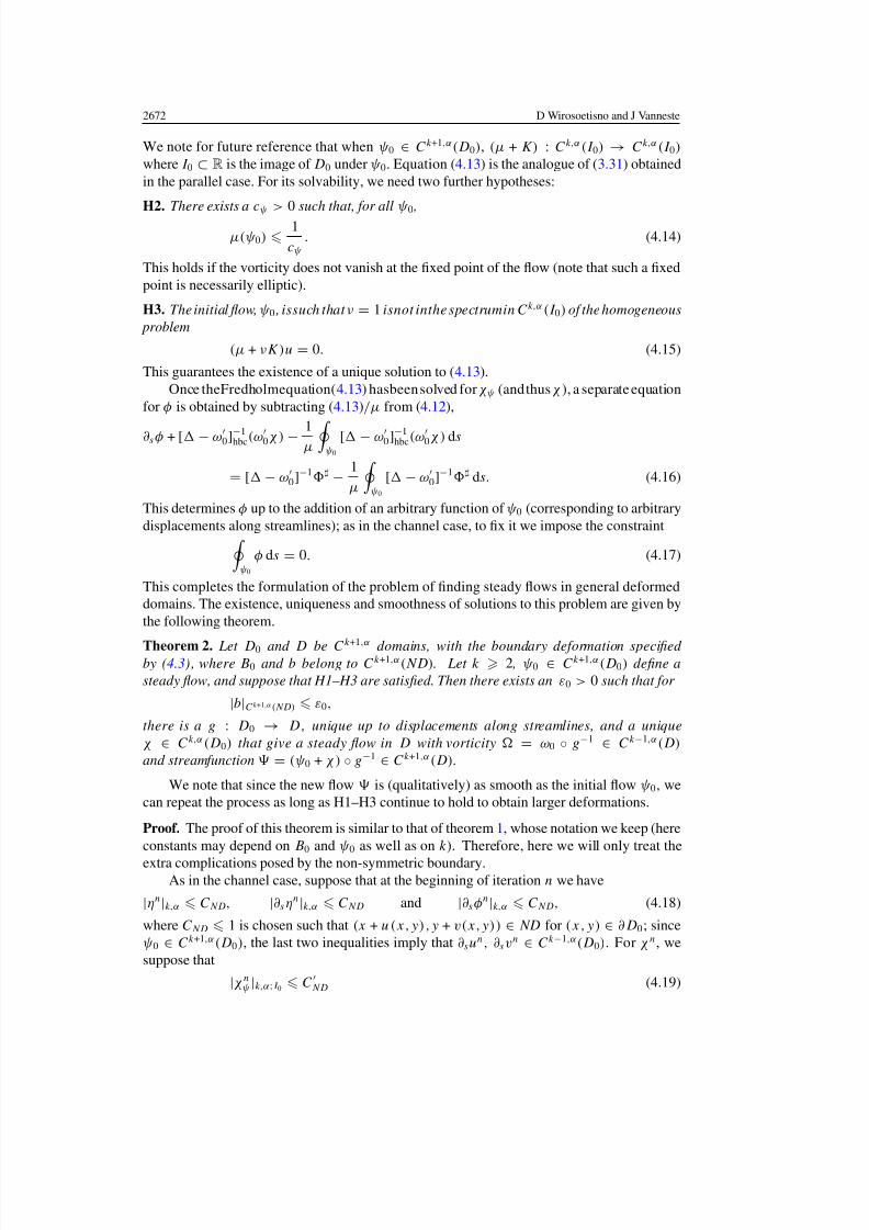
We note for future reference that when ψ0 ∈ Ck+1,α(D0), (µ + K) : Ck,α (I 0) → Ck,α (I 0)

where I 0 ⊂ R is the image of D0 under ψ0. Equation (4.13) is the analogue of (3.31) obtained

in the parallel case. For its solvability, we need two further hypotheses:

H2. There exists a cψ > 0 such that, for all ψ0 ,

µ(ψ0) 1

cψ

. (4.14)

This holds if the vorticity does not vanish at the fixed point of the flow (note that such a fixed

point is necessarily elliptic).

H3. The initial flow, ψ0 , issuch that ν = 1 isnot inthe spectrumin Ck,α (I 0) of the homogeneous

problem

(µ + νK)u = 0. (4.15)

This guarantees the existence of a unique solution to (4.13).

Once theFredholmequation(4.13) hasbeen solved forχψ (andthus χ ), a separate equation

for φ is obtained by subtracting (4.13)/µ from (4.12),

∂s φ + [ − ω0]−1

hbc(ω0χ ) − 1

µ

ψ0

[ − ω0]−1

hbc(ω0χ ) ds

= [ − ω0]−1 −

1

µ

ψ0

[ − ω0]−1 ds. (4.16)

This determines φ up to the addition of an arbitrary function of ψ0 (corresponding to arbitrary

displacements along streamlines); as in the channel case, to fix it we impose the constraint ψ0

φ ds = 0. (4.17)

This completes the formulation of the problem of finding steady flows in general deformed

domains. The existence, uniqueness and smoothness of solutions to this problem are given by

the following theorem.

Theorem 2. Let D0 and D be Ck+1,α domains, with the boundary deformation specified by (4.3) , where B0 and b belong to Ck+1,α(ND). Let k 2 , ψ0 ∈ Ck+1,α(D0) define a

steady flow, and suppose that H1–H3 are satisfied. Then there exists an ε0 > 0 such that for

|b|Ck+1,α (ND) ε0,

there is a g : D0 → D , unique up to displacements along streamlines, and a unique

χ ∈ Ck,α (D0) that give a steady flow in D with vorticity = ω0 ◦ g−1 ∈ Ck−1,α(D)

and streamfunction = (ψ0 + χ ) ◦ g−1 ∈ Ck+1,α(D).

We note that since the new flow is (qualitatively) as smooth as the initial flow ψ0, we

can repeat the process as long as H1–H3 continue to hold to obtain larger deformations.

Proof. The proof of this theorem is similar to that of theorem 1, whose notation we keep (here

constants may depend on B0 and ψ0 as well as on k). Therefore, here we will only treat the

extra complications posed by the non-symmetric boundary.As in the channel case, suppose that at the beginning of iteration n we have

|ηn|k,α CND, |∂s ηn|k,α CND and |∂s φn|k,α CND, (4.18)

where CND 1 is chosen such that (x + u(x,y),y + v(x,y)) ∈ ND for (x,y) ∈ ∂D0; since

ψ0 ∈ Ck+1,α(D0), the last two inequalities imply that ∂s un, ∂s vn ∈ Ck−1,α(D0). For χ n, we

suppose that

|χ nψ |k,α;I 0 C

ND (4.19)




and note that |χ |k,α c|χψ |k,α;I 0 ; we choose C ND such that |χ n|k,α CND. With a slight

abuse of notation we will henceforth write |χψ |k,α for |χψ |k,α;I 0 .

To estimate the boundary terms, we note using (3.21) that, since B0|∂D0= 0,

|B0 ◦ (id + u)|k,α;∂D0

c |B0|k,1;ND|u|k,α;∂D0

.

Using this to bound the first term in (4.5), bounding the second term in the obvious fashion

and using (3.22) to bound the last term, we arrive at

c|β(u,v; ·)|k,α;∂D0 |B0|k,1;ND|(u, v)|k,α;∂D0

+ |B0|k+1,α;∂D0|(u,v)|k,α;∂D0

+ |b|k,α;ND(1 + |(u,v)|k+αk,α;∂D0

). (4.20)

We estimate (u,v)|∂D0by ‘projection’ as in the channel case,

|u|k,α;∂D0 c|∂s u|k−1,α;∂D0

c|∂s u|k−1,α c(|∂s η|k,α + |∂s φ|k,α )

and a similar estimate for |v|k,α;∂D0. Introducing this into (4.20) and absorbing |B0|k+1,α;ND

into the constant, we arrive at

|β(u,v; ·)|k,α;∂D0 cb(1 + |∂s η|2

k,α;∂D0+ |∂s φ|2

k,α;∂D0), (4.21)

where b := |b|k,α;ND.As before, we compute ηn+1 by solving

ηn+1 = uny vn

x − unx vn

y in D0,

∂η n+1

∂n=

D0

[uny vn

x − unx vn

y ]dx dy

∂D0

dl on ∂D0.(4.22)

As in the channel case, here the boundary conditions are different from ( 4.7); however, upon

convergence these two boundary conditions are equivalent because both consist of a constant

which expresses the fact that g is area preserving. Lemma 2 then implies that

|ηn+1|k,α c(|φn|2k,α + |ηn|2

k,α ).

To bound ∂s ηn+1, we take ∂s (4.22a) and use the identity

( − ω0)∂s ϕ = ∂s ϕ + 2∇⊥∂x ψ0 · ∇∂x ϕ + 2∇⊥∂y ψ0 · ∇∂y ϕ

with ϕ = ηn+1. Noting that the entire right-hand side is bounded in Ck−2,α(D0) by

|ηn|2k,α + |∂s ηn|2

k,α + |∂s φn|2k,α , and using the argument leading to (3.29), lemma 2 again gives

|∂s ηn+1|k,α c1(|∂s φn|2k,α + |∂s ηn|2

k,α + |ηn|2k,α ). (4.23)

Now, the iteration corresponding to (4.9) is

χ n+1 + [ − ω0]∂s φn+1 = −2[ηn+1

xx ∂yy ψ0 + ηn+1yy ∂xx ψ0 − 2ηn+1

xy ∂xy ψ0] + nl(χ n, un, vn)

=: (χ n, un, vn; ηn+1). (4.24)

Thanks to the anisotropy of the nonlinear terms, nl, in (4.10), we have

|nl(φn, ηn, χ n)|k−2,α c(|∂s φn|2k,α + |∂s ηn|2

k,α + |ηn|2k,α + |χ n

ψ |2k,α ).

Combined with (4.23), the last line of (4.24) is bounded as

|(χ n, un, vn; ηn+1)|k−2,α c2(|∂s φn|2k,α + |∂s ηn|2

k,α + |ηn|2k,α + |χ n

ψ |2k,α ). (4.25)

Unlike in the proof of theorem 1, at this point we need to estimate the boundary

contribution, which is the solution, ∂s φn+1b , of the problem

[ − ω0]∂s φn+1

b = 0,

∂s φn+1b (x,y) = β(un, vn; x, y) (x, y) ∈ ∂D0.




Using (4.21),

|∂s φn+1b |k,α;∂D0

c(ψ0) b(1 + |∂s ηn|2k,α + |∂s φn|2

k,α ). (4.26)

Lemma 1 and (4.25) then give

|[ − ω0]−1

n |k,α c3(|∂s φn|2k,α + |∂s ηn|2

k,α + |ηn|2k,α + |χ n

ψ |2k,α + b), (4.27)

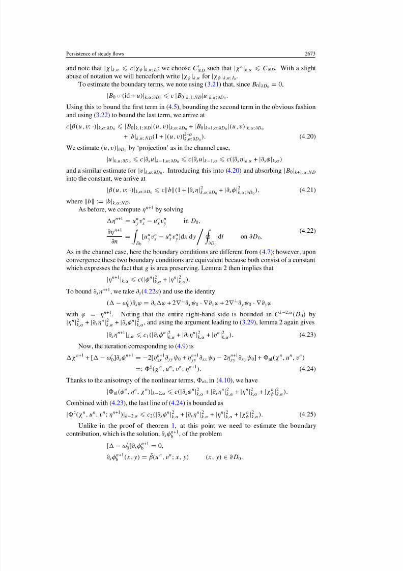
wherethe subscriptn on [ − ω0]−1 definedin(4.12), is a reminder that itsboundaryconditions

depend on (un, vn).

We turn to χ , obtained from (4.13),

(µ + K) χ n+1ψ (ψ0) =

ψ0

[ − ω0]−1

n (un, vn, χ n; ηn+1)ds =: (ψ0).

Using H2 and (4.27),

||Ck,α (I 0) c(ψ0)(|∂s φn|2k,α + |∂s ηn|2

k,α + |ηn|2k,α + |χ n

ψ |2k,α + b). (4.28)

Since by H3 the operator (µ + K) : Ck,α (I 0) → Ck,α (I 0) has a bounded inverse, we have

|χ n+1ψ |k,α c4(|∂s φn|2

k,α + |∂s ηn|2k,α + |ηn|2

k,α + |χ nψ |2

k,α + b). (4.29)

In the process we have bounded all the operators and the right-hand side in the iteration

corresponding to (4.16). Solving for φn+1, we find

|∂s φn+1|k,α c6(|∂s φn|2k,α + |∂s ηn|2

k,α + |ηn|2k,α + |χ n

ψ |2k,α + b). (4.30)

As in the channel case, boundedness of the iteration follows from (4.23), (4.29) and(4.30),

provided we take b sufficiently small. The convergence is very similar and we shall not do

it explicitly here.

Upon convergence, we have u, v ∈ Ck−1,α(D0) and so g−1 ∈ Ck−1,α(D,D0). Since

ω0 ∈ Ck−1,α(D0), this and (3.22) imply that = ω0 ◦ g−1 ∈ Ck−1,α(D), which in turn implies

that = −1 ∈ Ck+1,α(D).

Remarks. It is clear from (4.29) that χ is of the order of b, as is the linear solution χ 1; this

is to be contrasted with the channel case, where χ is quadratic in b (and where χ 1 = 0). As

in the channel case, φ ∼ O(b) (cf (4.30)) and η ∼ O(b2) (cf (4.23)).

5. Persistence of stability

If a steady flow persists when its domain boundary is deformed as established in the previous

sections, it is natural to ask whether its stability properties also persist. Of interest here is

the nonlinear stability of steady flows; it holds for a flow with vorticity and streamfunction

= F() if, in theevolutionof theperturbed flow +(t), a suitable norm of theperturbation

streamfunction |(t)| is bounded by |(0)| for all t .

For two-dimensionalincompressible and inviscid flows in general domains, useful stabilityresults of this type have been derived using the Arnold’s energy–Casimir method (Arnold

(1965, 1966); see also Holm et al (1985), Arnold and Khesin (1998)). The application of

this method provides two sufficient conditions for stability: the steady flow = F() is

nonlinearly stable if there are two constants c1 and c2 such that either

(i) 0 < c1 F c2 < ∞, or

(ii) 0 < λ1 < c1 −F c2 < ∞,




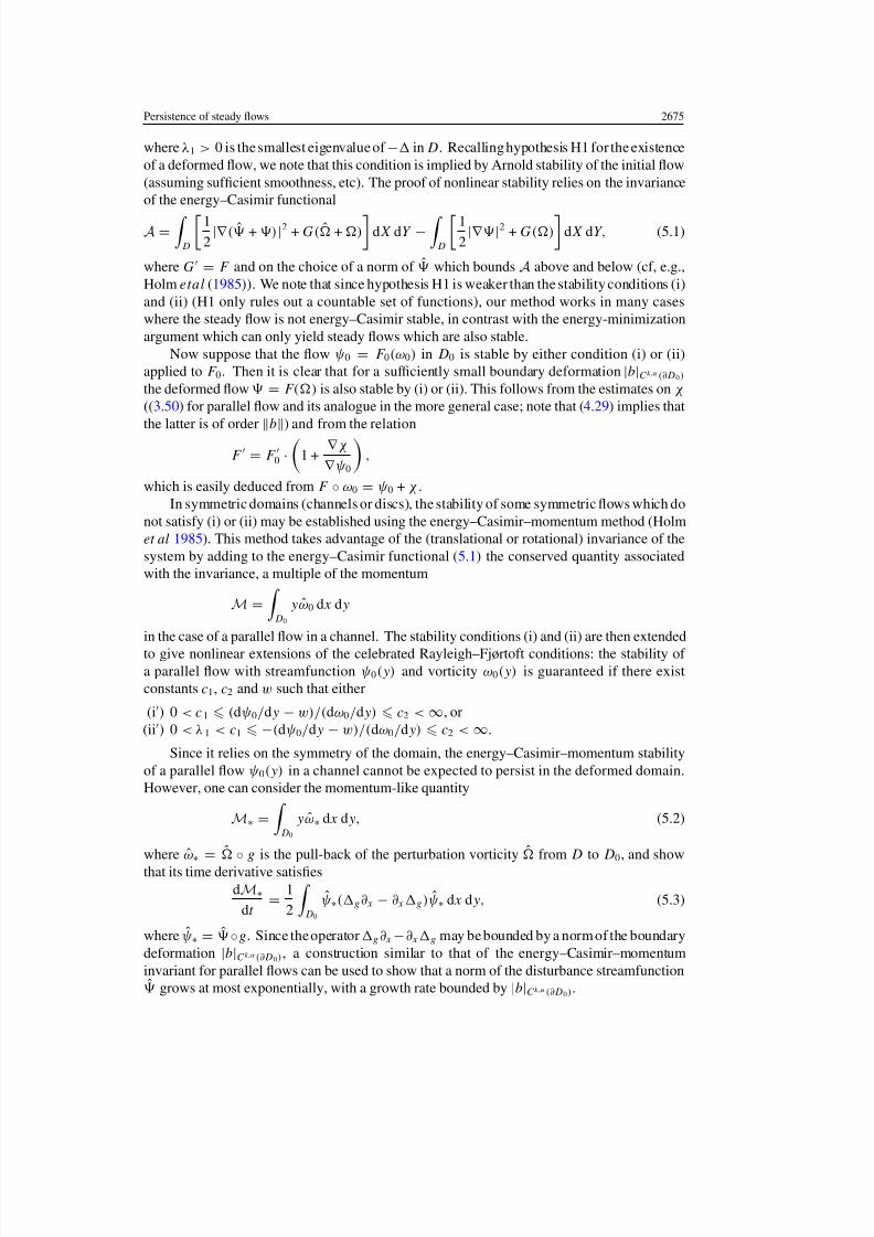
where λ1 > 0 is the smallest eigenvalue of − in D. Recalling hypothesis H1 for the existence

of a deformed flow, we note that this condition is implied by Arnold stability of the initial flow

(assuming sufficient smoothness, etc). The proof of nonlinear stability relies on the invariance

of the energy–Casimir functional

A =

D

1

2|∇( + )|2 + G( + )

dX dY −

D

1

2|∇|2 + G()

dX dY, (5.1)

where G = F and on the choice of a norm of which bounds A above and below (cf, e.g.,

Holm etal (1985)). We note that since hypothesis H1 is weaker than the stability conditions (i)

and (ii) (H1 only rules out a countable set of functions), our method works in many cases

where the steady flow is not energy–Casimir stable, in contrast with the energy-minimization

argument which can only yield steady flows which are also stable.

Now suppose that the flow ψ0 = F 0(ω0) in D0 is stable by either condition (i) or (ii)

applied to F 0. Then it is clear that for a sufficiently small boundary deformation |b|Ck,α (∂D0)

the deformed flow = F() is also stable by (i) or (ii). This follows from the estimates on χ

((3.50) for parallel flow and its analogue in the more general case; note that (4.29) implies that

the latter is of order b) and from the relation

F = F 0 ·

1 +

∇χ

∇ψ0

,

which is easily deduced from F ◦ ω0 = ψ0 + χ .

In symmetric domains (channels or discs), the stability of some symmetric flows which do

not satisfy (i) or (ii) may be established using the energy–Casimir–momentum method (Holm

et al 1985). This method takes advantage of the (translational or rotational) invariance of the

system by adding to the energy–Casimir functional (5.1) the conserved quantity associated

with the invariance, a multiple of the momentum

M =

D0

yω0 dx dy

in the case of a parallel flow in a channel. The stability conditions (i) and (ii) are then extended

to give nonlinear extensions of the celebrated Rayleigh–Fjørtoft conditions: the stability of a parallel flow with streamfunction ψ0(y) and vorticity ω0(y) is guaranteed if there exist

constants c1, c2 and w such that either

(i) 0 < c1 (dψ0/dy − w)/(dω0/dy) c2 < ∞, or

(ii) 0 < λ1 < c1 −(dψ0/dy − w)/(dω0/dy) c2 < ∞.

Since it relies on the symmetry of the domain, the energy–Casimir–momentum stability

of a parallel flow ψ0(y) in a channel cannot be expected to persist in the deformed domain.

However, one can consider the momentum-like quantity

M∗ =

D0

yω∗ dx dy, (5.2)

where ω∗ = ◦ g is the pull-back of the perturbation vorticity from D to D0, and show

that its time derivative satisfiesdM∗

dt =

1

2

D0

ψ∗(g∂x − ∂x g )ψ∗ dx dy, (5.3)

where ψ∗ = ◦g. Since the operator g ∂x −∂x g may be bounded by a norm of the boundary

deformation |b|Ck,α (∂D0), a construction similar to that of the energy–Casimir–momentum

invariant for parallel flows can be used to show that a norm of the disturbance streamfunction

grows at most exponentially, with a growth rate bounded by |b|Ck,α (∂D0).




6. A numerical example

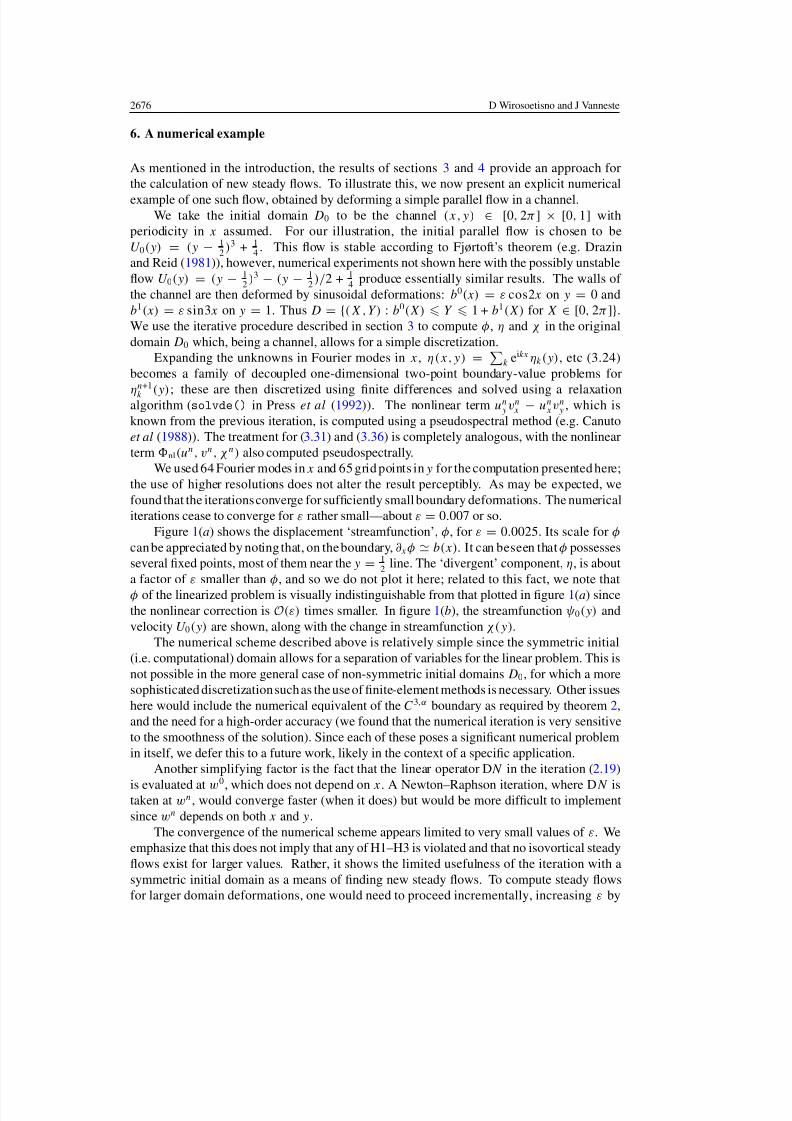
As mentioned in the introduction, the results of sections 3 and 4 provide an approach for

the calculation of new steady flows. To illustrate this, we now present an explicit numerical

example of one such flow, obtained by deforming a simple parallel flow in a channel.We take the initial domain D0 to be the channel (x,y) ∈ [0, 2π ] × [0, 1] with

periodicity in x assumed. For our illustration, the initial parallel flow is chosen to be

U 0(y) = (y − 12

)3 + 14

. This flow is stable according to Fjørtoft’s theorem (e.g. Drazin

and Reid (1981)), however, numerical experiments not shown here with the possibly unstable

flow U 0(y) = (y − 12

)3 − (y − 12

)/2 + 14

produce essentially similar results. The walls of

the channel are then deformed by sinusoidal deformations: b0(x) = ε cos2x on y = 0 and

b1(x) = ε sin3x on y = 1. Thus D = {(X,Y) : b0(X) Y 1 + b1(X) for X ∈ [0, 2π ]}.

We use the iterative procedure described in section 3 to compute φ, η and χ in the original

domain D0 which, being a channel, allows for a simple discretization.

Expanding the unknowns in Fourier modes in x, η(x,y) =

k eikx ηk (y), etc (3.24)

becomes a family of decoupled one-dimensional two-point boundary-value problems for

ηn+1

k (y); these are then discretized using finite differences and solved using a relaxationalgorithm (solvde() in Press et al (1992)). The nonlinear term un

y vnx − un

x vny , which is

known from the previous iteration, is computed using a pseudospectral method (e.g. Canuto

et al (1988)). The treatment for (3.31) and (3.36) is completely analogous, with the nonlinear

term nl(un, vn, χ n) also computed pseudospectrally.

We used 64 Fourier modes in x and 65 grid points in y for the computation presented here;

the use of higher resolutions does not alter the result perceptibly. As may be expected, we

found that the iterations converge for sufficiently small boundary deformations. The numerical

iterations cease to converge for ε rather small—about ε = 0.007 or so.

Figure 1(a) shows the displacement ‘streamfunction’, φ, for ε = 0.0025. Its scale for φ

can be appreciated by noting that, on the boundary, ∂x φ b(x). It can beseen that φ possesses

several fixed points, most of them near the y = 12

line. The ‘divergent’ component, η, is about

a factor of ε smaller than φ, and so we do not plot it here; related to this fact, we note that

φ of the linearized problem is visually indistinguishable from that plotted in figure 1(a) since

the nonlinear correction is O(ε) times smaller. In figure 1(b), the streamfunction ψ0(y) and

velocity U 0(y) are shown, along with the change in streamfunction χ(y).

The numerical scheme described above is relatively simple since the symmetric initial

(i.e. computational) domain allows for a separation of variables for the linear problem. This is

not possible in the more general case of non-symmetric initial domains D0, for which a more

sophisticated discretization such as the use of finite-element methods is necessary. Other issues

here would include the numerical equivalent of the C3,α boundary as required by theorem 2,

and the need for a high-order accuracy (we found that the numerical iteration is very sensitive

to the smoothness of the solution). Since each of these poses a significant numerical problem

in itself, we defer this to a future work, likely in the context of a specific application.

Another simplifying factor is the fact that the linear operator DN in the iteration (2.19)

is evaluated at w0, which does not depend on x. A Newton–Raphson iteration, where DN istaken at wn, would converge faster (when it does) but would be more difficult to implement

since wn depends on both x and y.

The convergence of the numerical scheme appears limited to very small values of ε. We

emphasize that this does not imply that any of H1–H3 is violated and that no isovortical steady

flows exist for larger values. Rather, it shows the limited usefulness of the iteration with a

symmetric initial domain as a means of finding new steady flows. To compute steady flows

for larger domain deformations, one would need to proceed incrementally, increasing ε by




Figure 1. Deformation of a parallel flow. The basic flow has U 0(y) = (y − 12

)3 + 14 , and the

boundary deformation is defined by b0(x) = ε cos2x and b1(x) = ε sin 3x with ε = 0.0025.

(a) Top panel: contour plot of the displacement streamfunction φ( x,y) in the channel. Contourlevel is 2 × 10−4. (b) Bottom panel: change in the streamfunction χ(y), magnified by 104, initialstreamfunction ψ0(y) and velocity U 0(y).

small steps and using the flow computed at each step as the intial flow for the next step.

This, of course, is numerically much more involved since it requires an implementation for

non-symmetric initial domains.

A possible explanation for the smallness of ε required for the convergence of our iteration

(analytical and numerical) is the following: suppose that a steady flow ω0 in domain D0 is

continuously deformable to in D without violating H1–H3. A given path γ connecting D0

and D in the space of domains then defines a path of steady flows connecting ω0 and in the

space of isovortical flows (equivalently, one may take to live in the space of area-preserving

diffeomorphisms with g0

: D0

→ D0

and g : D0

→ D). Now there is a neighbourhood of

outside which our iteration fails to converge, and so if is significantly ‘curved’, small steps

(i.e. repeated applications of theorem 2) are needed in order to remain in this neighbourhood.

7. Discussion and future work

In section 3 we haveshown that a parallel flow persists as a steadyflow under finite deformations

of its channel domain. Apart from sufficient smoothness, the only hypothesis required is that




the velocity does not vanish anywhere. A similar computation shows that this result also holds

for an axisymmetric flow, provided that the velocity vanishes only at the centre of the disc,

where the vorticity cannot be zero (cf the comment following H2). For the more general case

of a non-symmetric flow discussed in section 4, hypothesis H2 can be viewed as the natural

extension of this constraint on the non-vanishing of the velocity; but two additional hypotheses,H1 and H3, are necessary for our proof of the existence and uniqueness of a steady deformed

flow. There appears, therefore, to be a significant difference between the symmetric (parallel

or axisymmetric) and non-symmetric cases.

It is easy to understand why H1, i.e. the invertibility of − ω0, is not needed explicitly

in the symmetric cases: it is a direct consequence of the non-vanishing of the velocity. As

the following calculation shows for the parallel case, if − ω0 has a nontrivial homogeneous

solution, U 0 must vanish somewhere,

( − ω0)φ = [ − (∂yy U 0/U 0)]φ = 0 ⇔ ∇ · [U 20 ∇(φ/U 0)] = 0

⇒

U 20 |∇(φ/U 0)|2 dy = 0 (7.1)

(cf Howard (1961)). In view of this, it is natural to ask whether an analogous result holds in

the general, non-symmetric case, that is, whether H2 generally implies H1. We have not beenable to establish this. The precise role and physical significance of H3 still elude us at the

moment.

Note thatthereis an importantdifference between the symmetric and non-symmetric flows:

the change in the streamfunction χ is quadratic in b in the symmetric case but is linear in

b in general. This shows that a symmetric flow is a critical point of the ω–ψ relationship in

the sense that, using ε as a parameter for a domain deformation ‘path’, dF /dε = 0 as the path

passes through a symmetric domain.

As mentioned in the introduction, one of the interests of the isovortical steady flows

considered in this paper is that they can be achieved at least approximately by an adiabatically

slow deformation of thefluid domain. In this context, an intriguing question concerns thenature

of the flow evolution when an isovortical steady flow does not exist. We might speculate that

in such a case the adiabatic deformation of the domain leads to a complex transient flow,even at leading order. This is suggested by the behaviour of parallel flows whose velocity

vanishes somewhere so that theorem 1 does not apply. When disturbed, these flows, even

when Arnold stable, exhibit complicated transient dynamics associated with the formation

of a critical layer (Stewartson 1978, Warn and Warn 1978). This phenomenon confirms the

importance of assuming a non-vanishing velocity to ensure the persistence of steady parallel

flows. Viewing H2 as the natural extension to non-parallel flows of this assumption, one might

conjecture that a physical phenomenon similar to a critical layer occurs in flows for which H2

is violated, i.e. in flows for which dl

|∇ψ0|= ∞ (7.2)

for some streamline. The dynamics in such non-parallel flows is certainly worth investigating.

It should be noted, moreover, that the presence of a stagnation point, where ∇ψ0 = 0 and H2is violated, is known to lead to some form of instability (Friedlander and Vishik 1992, Vishik

1996).

Acknowledgments

This work was funded by an EPSRC research grant, and by a William Gordon Seggie Brown

Fellowship held by DW at the University of Edinburgh. Additional support was provided by




the EPSRC Network ‘Geometric methods in geophysical fluid dynamics’. JV is supported by

a NERC Advanced Fellowship. We thank C Foias, J-M Rakotoson and R Temam for helpful

comments and discussions, and thank the anonymous referees for constructive comments and

suggestions.

Appendix. Summary of notation

Let g : D0 → D : (x,y) → (X,Y) = (x + u(x,y),y + v(x,y)) = (x,y) + ∇η(x,y) +

∇ ⊥φ(x,y). Then we have:

Object Original domain D0 Deformed domain D

Coordinates (x, y) (X, Y )

Vorticity ω0 := ω0 ◦ g−1

Streamfunction ψ0 = F 0 ◦ ω0 = F ◦

Pulled-back streamfunction ψ∗ := ◦ g

=: ψ0 + χ

Pulled-back (for f : D0 → R) gf := [(f ◦ g−1)] ◦ g (f ◦ g−1)

Primes denote derivative with respect to ψ0:

ω0 := ∇ω0/∇ψ0 = (F −1

0 ) ◦ ω0, ψ ∗ := ∇ψ∗/∇ψ0 and χ := ∇χ /∇/ψ0.

References

Arnold V I 1965 Dokl. Akad. Nauk SSSR 162 975–8 (in Russian)

Arnold V I 1965 Conditions for nonlinear stability of stationary plane curvilinear flows of an ideal fluid Sov. Math. 6

773–7 (Engl. Transl.)

Arnold V I 1966 Izv. Vyssh. Uchebn. Zaved. Mat. 53 3–5 (in Russian)

Arnold V I 1966 On an a priori estimate in the theory of hydrodynamical stability Am. Math. Soc. Transl. Ser. 2 79

267–9 (Engl. Transl.)

Arnold V I and Khesin B A 1998 Topological Methods in Hydrodynamics (Berlin: Springer) xvi + 374 pp

Canuto C, Hussaini M Y, Quarteroni A and Zang T A 1988 Spectral Methods in Fluid Dynamics (Berlin: Springer)

xvi+ 557 pp

Crowdy D G 1997 General solutions to the 2D Liouville equation Int. J. Eng. Sci. 35 141–9

de la Llave R and Obaya R 1999 Regularity of the composition operator in spaces of Holder functions Discrete Cont.

Dyn. Syst. 5 157–84

Drazin P G and Reid W H 1981 Hydrodynamic Stability (Cambridge: Cambridge University Press) xiv + 527 pp

Friedlander S and Vishik M M 1992 Instability criteria for steady flows of a perfect fluid Chaos 2 455–60

Gilbarg D andTrudingerN S 1977 Elliptic Partial DifferentialEquations of SecondOrder (Berlin:Springer) x + 401 pp

Holm D D, Marsden J E, Ratiu T S and Weinstein A 1985 Nonlinear stability of fluid and plasma equilibria Phys.

Rep. 123 1–116

Howard L N 1961 Note on a paper by John W Miles J. Fluid Mech. 10 509–12

Kolmogorov A N and Fomin S V 1970 Introductory Real Analysis transl and ed R A Silverman (New York: Dover)

xii+ 403 pp

Kuzin I and Pokhozhaev S I 1997 Entire Solutions of Semilinear Elliptic Equations (Basel: Birkhauser) vi+ 250 pp

Ladyzhenskaya O A and Ural’tseva, N N 1968 Linear and Quasilinear Elliptic Equations (New York: Academic)

xviii+ 495 pp

Mallier R and Maslowe S A 1993 A row of counter-rotating vortices Phys. Fluids A 5 1074–5

MoffattH K 1992Relaxationunder topological constraints Topological Aspects of the Dynamics of Fluidsand Plasmas

ed H K Moffatt et al (Dordrecht: Kluwer) pp 3–28

Pokhozhaev S I 1965 Dokl. Akad. Nauk SSSR 165 36–9

Pokhozhaev S I 1965 Eigenfunctions of the equation u + λf (u) = 0 Sov. Math. 6 1408–1 (Engl. Transl.)




Press W H, Teukolsky S A, Vetterling W T and Flannery B P 1992 Numerical Recipes in C 2nd edn (Cambridge:

Cambridge University Press) xxvi + 994 pp

Shepherd T G 1990A general method for finding extremalstates of Hamiltonian dynamical systems, with applications

to perfect fluids J. Fluid Mech. 213 573–87

Shnirelman A 1993 Lattice theory and flows of ideal incompressible fluid Russ. J. Math. Phys. 1 105–14

Stewartson K 1978 The evolution of the critical layer of a Rossby wave Geophys. Astrophys. Fluid Dyn. 9 185–200

Stuart J T 1967 On finite amplitude oscillations in laminar mixing layers. J. Fluid Mech. 29 417–40

Taylor M E 1996 Partial Differential Equations III: Nonlinear Equations (Berlin: Springer) xxii + 608 pp

Vishik M 1996 Spectrum of small oscillations of an ideal fluid and Lyapunov exponents J. Math. Pures Appl. 75

531–57

Warn T and Warn H 1978 The evolution of a nonlinear critical level Stud. Appl. Math. 59 37–71

Date post:	06-Apr-2018
Category:	Documents
Upload:	pelaggio
View:	220 times
Download:	0 times

D Wirosoetisno and J Vanneste- Persistence of steady flows of a two-dimensional perfect fluid in...

Documents