IOSR Journal of Engineering (IOSRJEN) www.iosrjen.org

ISSN (e): 2250-3021, ISSN (p): 2278-8719

Vol. 05, Issue 07 (July. 2015), ||V4|| PP 13-25

International organization of Scientific Research 13 | P a g e

Modeling and Optimization of the Poison’s Ratio of Latertic

Concrete using Scheffe’s Theory

1Onuamah, P.N. and

2Osadebe N. N.

1. Civil Engineering Department, Enugu State University of Science and Technology, Enugu, Nigeria.

2. Civil Engineering Department, University of Nigeria,Nsukka.

ABSTRACT: The ubiquity of laterite in this region of the world imposes the need for its utilization in concrete

and road making works for the economic growth of the region. Laterite is the reddish soil layer often belying the

top soil in many locations and further deeper in some areas, collected from the Vocational Education Building

Site of the University of Nigeria, Nsukka. The paper presents the report of an investigation carried out to model

and optimize the Poison ratio of Lateritic Concrete. The work applied the Scheffe’s optimization approach to

obtain a mathematical model of the form f(xi1,xi2,xi3), where xi are proportions of the concrete components, viz:

cement, laterite and water. Scheffe’s experimental design techniques are followed to mould various block

samples measuring 220mm x 210mm x 120mm, with varying generated components ratios which were tested

for 28 days strength to obtain the model: Ŷc = 0.33X1+ 0.27X2 + 0.45X3 + 0.52X1X2 – 0.02X2X3 . To carry out

the task, we embark on experimentation and design, applying the second order polynomial characterization

process of the simplex lattice method. The model adequacy is checked using the control factors. Finally a

software is prepared to handle the design computation process to select the optimized properties of the mix, and

generate the optimal mix ratios for the desired property.

Keywords: Optimization, Lateritic concrete, pseudo-component, Simplex-lattice, model adequacy.

I. INTRODUCTION

In the present time, concrete is the main material of construction, and the ease or cost of its production

accounts for the level of success in the of area environmental upgrading through the construction of new roads,

buildings, dams, water structures and the renovation of such structures. To produce the concrete several primary

components such as cement, sand, gravel and some admixtures are to be present in varying quantities and

qualities. Unfortunately, the occurrence and availability of these components vary very randomly with location

and hence the attendant problems of either excessive or scarce quantities of the different materials occurring in

different areas. Where the scarcity of one component prevails exceedingly, the cost of the concrete production

increases geometrically. Such problems obviate the need to seek alternative materials for partial or full

replacement of the component when it is possible to do so without losing the quality of the concrete [1].

The construction of structures is a regular operation which creates the opportunity for continued change

and improvement on the face of the environment. From the beginning of time, the cost of this change has been

of major concern to man as the major construction factors are finance, labour, materials and equipment.

Major achievements in the area of environmental development is heavily dependent on the availability

of construction materials which take a high proportion of the cost of the structure. This means that the locality

of the material and the usability of the available materials directly impact on the achievable development of the

area as well as the attainable level of technology in the area.

Concept of Optimization In every business the success plan is to achieve low output/input index. The target of planning is the

maximization of the desired outcome of the venture. In order to maximize gains or outputs it is often necessary

to keep inputs or investments at a minimum at the production level. The process involved in this planning

activity of minimization and maximization is referred to as optimization [2]. In the science of optimization, the

desired property or quantity to be optimized is referred to as the objective function. The raw materials or

quantities whose amount of combinations will produce this objective function are referred to as variables.

The variations of these variables produce different combinations and have different outputs. Often the

space of variability of the variables is not universal as some conditions limit them. These conditions are called

constraints. For example, money is a factor of production and is known to be limited in supply. The constraint at

any time is the amount of money available to the entrepreneur at the time of investment.

Hence or otherwise, an optimization process is one that seeks for the maximum or minimum value and at the

same time satisfying a number of other imposed requirements [3].

Modeling and Optimization of the Poison’s Ratio of Latertic Concrete using Scheffe’s Theory

International organization of Scientific Research 14 | P a g e

The function is called the objective function and the specified requirements are known as the

constraints of the problem.

Making structural concrete is not all comers' business. Structural concrete are made with specified materials for

specified strength. Concrete is heterogeneous as it comprises sub-materials. Concrete is made up of fine

aggregates, coarse aggregates, cement, water, and sometimes admixtures. Researchers [4] report that modern

research in concrete seeks to provide greater understanding of its constituent materials and possibilities of

improving its qualities. For instance, Portland cement has been partially replaced with ground granulated blast

furnace slag (GGBS), a by–product of the steel industry that has valuable cementations properties [5].

Bloom and Bentur [6] reports that optimization of mix designs require detailed knowledge of concrete

properties. Low water-cement ratios lead to increased strength but will negatively lead to an accelerated and

higher shrinkage. Apart from the larger deformations, the acceleration of dehydration and strength gain will

cause cracking at early ages.

Modeling

Modeling has to do with formulating equations of the parameters operating in the physical or other systems.

Many factors of different effects occur in nature in the world simultaneously dependently or independently.

When they interplay they could inter-affect one another differently at equal, direct, combined or partially

combined rates variationally, to generate varied natural constants in the form of coefficients and/or exponents

[6]. The challenging problem is to understand and asses these distinctive constants by which the interplaying

factors underscore some unique natural phenomenon towards which their natures tend, in a single, double or

multi phase system.

A model could be constructed for a proper observation of response from the interaction of the factors through

controlled experimentation followed by schematic design where such simplex lattice approach [7]. Also entirely

different physical systems may correspond to the same mathematical model so that they can be solved by the

same methods. This is an impressive demonstration of the unifying power of mathematics [8].

II. LITERATURE REVIEW The mineralogical and chemical compositions of laterites are dependent on their parent rocks [9].

Laterite formation is favoured in low topographical reliefs of gentle crests and plateaus which prevent the

erosion of the surface cover [10].

Of all the desirable properties of hardened concrete such as the tensile, compressive, flexural, bond,

shear strengths, etc., the compressive strength is the most convenient to measure and is used as the criterion for

the overall quality of the hardened concrete [3]. To be a good structural material, the material should be

homogeneous and isotropic. The Portland cement, laterite or concrete are none of these, nevertheless they are

popular construction materials [11]. With given proportions of aggregates the compressive strength of concrete

depends primarily upon age, cement content, and the cement-water ratio [12].

Simplex is a structural representation (shape) of lines or planes joining assumed positions or points of

the constituent materials (atoms) of a mixture, and they are equidistant from each other [13] When studying the

properties of a q-component mixture, which are dependent on the component ratio only the factor space is a

regular (q-1)–simplex [14]. Simplex lattice designs are saturated, that is, the proportions used for each factor

have m + 1 equally spaced levels from 0 to 1 (xi = 0, 1/m, 2/m, … 1), and all possible combinations are derived

from such values of the component concentrations, that is, all possible mixtures, with these proportions are used

[14].

Theoretical Background

This is a theory where a polynomial expression of any degree is used to characterize a simplex lattice

mixture components. In the theory only a single phase mixture is covered. The theory lends path to a unifying

equation model capable of taking varying components ratios to fix approximately equal mixture properties. The

optimization process goes to avail optimal ratios, from which selection can be made based on economic or

strength criteria. The theory is adapted to this work on the formulation of response function for Poison’s ratio of

lateritic concrete with laterite as the sole aggregate.

Simplex Lattice

Simplex is a structural representation (shape) of lines or planes joining assumed positions or points of

the constituent materials (atoms) of a mixture [13], and they are equidistant from each other. Mathematically, a

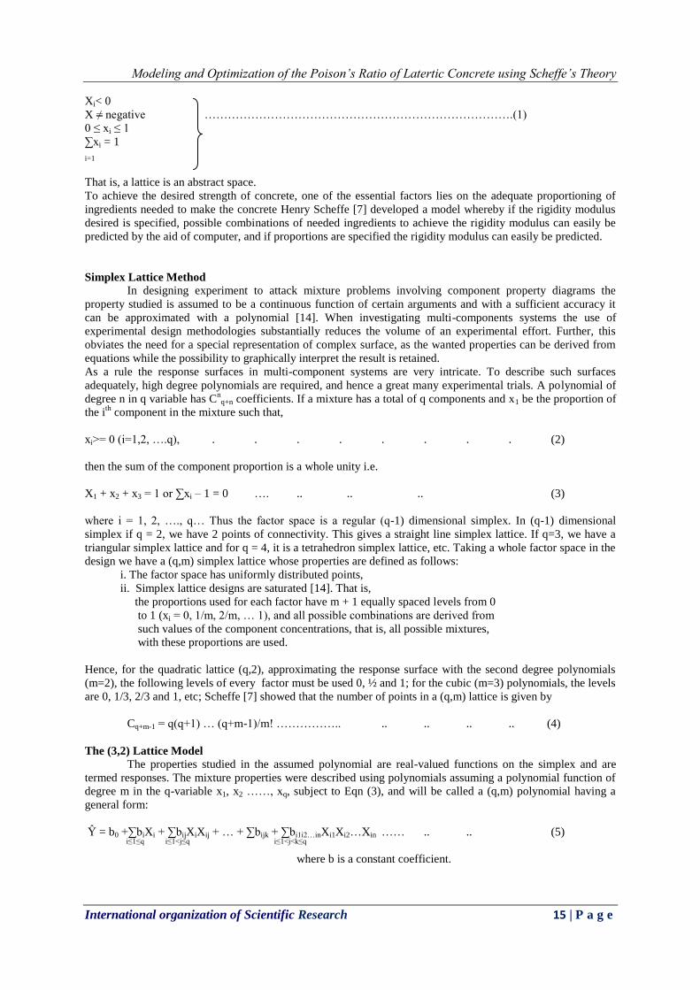
simplex lattice is a space of constituent variables of X1, X2, X3,……, and Xi which obey these laws:

Modeling and Optimization of the Poison’s Ratio of Latertic Concrete using Scheffe’s Theory

International organization of Scientific Research 15 | P a g e

Xi< 0

X ≠ negative …………………………………………………………………….(1)

0 ≤ xi ≤ 1

∑xi = 1

i=1

That is, a lattice is an abstract space.

To achieve the desired strength of concrete, one of the essential factors lies on the adequate proportioning of

ingredients needed to make the concrete Henry Scheffe [7] developed a model whereby if the rigidity modulus

desired is specified, possible combinations of needed ingredients to achieve the rigidity modulus can easily be

predicted by the aid of computer, and if proportions are specified the rigidity modulus can easily be predicted.

Simplex Lattice Method

In designing experiment to attack mixture problems involving component property diagrams the

property studied is assumed to be a continuous function of certain arguments and with a sufficient accuracy it

can be approximated with a polynomial [14]. When investigating multi-components systems the use of

experimental design methodologies substantially reduces the volume of an experimental effort. Further, this

obviates the need for a special representation of complex surface, as the wanted properties can be derived from

equations while the possibility to graphically interpret the result is retained.

As a rule the response surfaces in multi-component systems are very intricate. To describe such surfaces

adequately, high degree polynomials are required, and hence a great many experimental trials. A polynomial of

degree n in q variable has Cn

q+n coefficients. If a mixture has a total of q components and x1 be the proportion of

the ith

component in the mixture such that,

xi>= 0 (i=1,2, ….q), . . . . . . . . (2)

then the sum of the component proportion is a whole unity i.e.

X1 + x2 + x3 = 1 or ∑xi – 1 = 0 …. .. .. .. (3)

where i = 1, 2, …., q… Thus the factor space is a regular (q-1) dimensional simplex. In (q-1) dimensional

simplex if q = 2, we have 2 points of connectivity. This gives a straight line simplex lattice. If q=3, we have a

triangular simplex lattice and for q = 4, it is a tetrahedron simplex lattice, etc. Taking a whole factor space in the

design we have a (q,m) simplex lattice whose properties are defined as follows:

i. The factor space has uniformly distributed points,

ii. Simplex lattice designs are saturated [14]. That is,

the proportions used for each factor have m + 1 equally spaced levels from 0

to 1 (xi = 0, 1/m, 2/m, … 1), and all possible combinations are derived from

such values of the component concentrations, that is, all possible mixtures,

with these proportions are used.

Hence, for the quadratic lattice (q,2), approximating the response surface with the second degree polynomials

(m=2), the following levels of every factor must be used 0, ½ and 1; for the cubic (m=3) polynomials, the levels

are 0, 1/3, 2/3 and 1, etc; Scheffe [7] showed that the number of points in a (q,m) lattice is given by

Cq+m-1 = q(q+1) … (q+m-1)/m! …………….. .. .. .. .. (4)

The (3,2) Lattice Model

The properties studied in the assumed polynomial are real-valued functions on the simplex and are

termed responses. The mixture properties were described using polynomials assuming a polynomial function of

degree m in the q-variable x1, x2 ……, xq, subject to Eqn (3), and will be called a (q,m) polynomial having a

general form:

Ŷ = b0 +∑biXi + ∑bijXiXij + … + ∑bijk + ∑bi1i2…inXi1Xi2…Xin …… .. .. (5)

i≤1≤q i≤1<j≤q i≤1<j<k≤q

where b is a constant coefficient.

Modeling and Optimization of the Poison’s Ratio of Latertic Concrete using Scheffe’s Theory

International organization of Scientific Research 16 | P a g e

q

X=1

q

The relationship ∑xi = 1 enables the qth

component to be eliminated and the number of coefficients reduced to

Cm

q+m-1, but the very character of the problem dictates that all the q components be introduced into the model.

Substituting into equation Eqn (5), the polynomial has the general usable form:

Ŷ = b0 +b1X1 + b2X2 + b3X3 + b12X1X2 + b13X1X13 + b23X2X3 +

b11X21 + b22X

22 + b33X

23 …… ….. … (6)

By applying the normalization condition of Eqn. (3) and to Eqn (6) and jogling [6], we get that

Ŷ = β1X1+ β2X2 + β3X3 + β12X1X2+ β13X1X3 + β23X2X23 . . ( 7)

where

βi = b0 + bi + bii and βij = bij - bii - bjj, . . . . . (8)

Thus, the number of coefficients has reduced from 10 in Eqn (6) to 6 in Eqn (7). That is, the reduced second

degree polynomial in q variables is

Ŷ = ∑ βiXi +∑βijXi .. .. .. .. .. .. (9)

Construction of Experimental/Design Matrix

From the coordinates of points in the simplex lattice, we can obtain the design matrix. We recall that

the principal coordinates of the lattice, only a component is 1, others are zero (Table 1).

Hence if we substitute in Eqn. (7), the coordinates of the first point (X1=1, X2=0, and X3=0, Table 1), we get

that Y1= β1.

And doing so in succession for the other two points if the hexahedron, we obtain

Y2= β2,Y3= β3 .. . . . . . . (10)

\

The substitution of the coordinates of the fourth point yields

Y12 = ½ X1 + ½X2 + ½X1.X2

= ½ β1 + ½ β 2 + 1/4 β12

But as βi = Yi then

Y12 = ½ β1 - ½ β 2 - 1/4 β12

Thus

β12 = 4 Y12 - 2Y1 - 2Y2 . . . . .

And similarly,

β13 = 4 Y13 - 2Y1 - 2Y2

β23 = 4 Y23 - 2Y2 - 2Y3

Or generalizing,

βi = Yiand βij = 4 Yij - 2Yi - 2Yj . . . . . . .(11)

which are the coefficients of the reduced second degree polynomial for a q-component mixture, since the three

points defining the coefficients βij lie on the edge. The subscripts of the mixture property symbols indicate the

relative content of each component Xi alone and the property of the mixture is denoted by Yi. Mixture 4 includes

X1 and X2, and the property being designated Y12.

Actual and Pseudo Components

The requirements of the simplex that ∑ Xi = 1 makes it impossible to use the normal mix ratios

such as 1:3, 1:5, etc, at a given water/cement ratio. Hence a transformation of the actual components (ingredient

proportions) to meet the above criterion is unavoidable. Such transformed ratios say X1(i)

, X2(i)

, and X3(i)

for the

ith

experimental points are called pseudo components. Since X1, X2 and X3 are subject to ∑ Xi = 1, the

transformation of cement:laterite:water at say 0.60 water/cement ratio cannot easily be computed because X1, X2

and X3 are in pseudo expressions X1(i)

, X2(i)

, and X3(i)

. For the ith

experimental point, the transformation

computations are to be done.

Modeling and Optimization of the Poison’s Ratio of Latertic Concrete using Scheffe’s Theory

International organization of Scientific Research 17 | P a g e

The arbitrary vertices chosen on the triangle are A1(1:7.50:0.05), A2(1:8.20:0.03) and A3(1:6.90:0.10), based on

experience and earlier research reports.

Transformation Matrix

If Z denotes the actual matrix of the ith

experimental points, observing from Table 1 (points 1 to 3),

BZ = X =1 . . . . . . . . . . (12)

where B is the transformed matrix.

Therefore, B = I.Z-1

Or B=Z-1

. . . . . . . . (13)

For instance, for the chosen ratios, at the vertices A1, A2 and A3,

1.00 7.50 0.50

Z = 1.00 8.20 0.30 . . . . . . (14)

1.00 6.90 0.10

From Eqn (13),

B =Z-1

26.65 -17.60 -8.04

Z-1

= -30.04 2.17 0.87

-56.52 26.08 30.43

Hence,

1 0 0

B Z-1

= Z. Z-1

= 0 1 0

0 0 1

Thus, for actual component Z, the pseudo component X is given by

X1(i)

26.65 -17.60 -8.04 Z1(i)

X X2(i)

= B -30.04 2.17 0.87 Z Z2(i)

X3(i)

-56.52 26.08 30.43 Z3(i)

which gives the Xi(i=1,2,3) values in Table 1.

The inverse transformation from pseudo component to actual component is expressed as

AX = Z . . . . . . . . . (15)

where A = inverse matrix

A = Z X-1

.

From Eqn 3.16, X = BZ, therefore,

A = Z. (BZ)-1

A = Z.Z

-1B

-1

A = IB

-1

B = B

-1 . . . . . . . . .

(16)

This implies that for any pseudo component X, the actual component is given by

Z1(i)

1 7.50 0.05 X1(i)

Z Z2(i)

= B 1 8.20 0.03 X X2(i)

. . . . .

(17)

Z3(i)

1 6.9 0.10 X3(i)

Eqn (17) is used to determine the actual components from points 4 to 6 , and the control values from points 7 to

9 (Table 1).

Modeling and Optimization of the Poison’s Ratio of Latertic Concrete using Scheffe’s Theory

International organization of Scientific Research 18 | P a g e

i

i

n

Table 1 Values for Experiment N X1 X2 X3 RESPONSE Z1 Z2 Z3

1 1 0 0 Y1 1 1 1

2 0 1 0 Y2 7.50 8.20 6.90

3 0 0 1 Y3 0.05 0.03 0.10

4 1/2 1/2 0 Y12 1 7.85 0.04

5 ½ 0 1/2 Y13 1 7.20 0.075

6 0 1/2 1/2 Y23 1 7.55 0.065

Control Points (7-9)

7 1/3 1/3 1/3 Y123 1 7.458 0.0594

8 1/3 2/3 0 Y122 1 7.698 0.0366

9 0 1/3 2/3 Y233 1 7.329 0.0769

Use of Values in Experiment

During the laboratory experiment, the actual components were used to measure out the appropriate

proportions of the ingredients: cement, laterite and water, for mixing the lateritic concrete materials for casting

the samples. The values obtained are presented in Tables in section 5.

III. METHODOLOGY

Materials

The disturbed samples of laterite material were collected at the Vocational Education project site at the

University of Nigeria, Nsukka, at the depth of 1.5m below the surface.

The water for use is pure drinking water which is free from any contamination i.e. nil Chloride content, pH =6.9,

and Dissolved Solids < 2000ppm. Ordinary Portland cement is the hydraulic binder used in this project and

sourced from the Dangote Cement Factory, and assumed to comply with the Standard Institute of Nigeria (NIS)

1974, and kept in an air-tight bag.

Material Properties

All samples of the laterite material conformed to the engineering properties already determined by a

team of engineering consultants from the Civil Engineering Department, U.N.N, who reported on the Sieve

Analysis Tests, Natural Moisture Content, etc, carried out according to the British Standard Specification, BS

1377 – “Methods of Testing Soils for Civil Engineering Purposes”.

Preparation of Samples

The sourced materials for the experiment were transferred to the laboratory where they were allowed to

dry. A samples of the laterite were prepared and tested to obtain the moisture content for use in proportioning

the components of the lateritic concrete to be prepared. The laterite was sieved to remove debris and coarse

particles. The component materials were mixed at ambient temperature. The materials were mixed by weight

according to the specified proportions of the actual components generated in Table 1. In all, two blocks of

220mm x210 x120mm for each of six experimental points and three control points were cast for the rigidity

modulus test, cured for 28 days after setting and hardening.

Strength Test

After 28 day of curing, the cubes and blocks were crushed, with dimensions measured before and at

the point of shearing, to determine the lateritic concrete block strength, using the compressive testing machine to

the requirements of BS 1881:Part 115 of 1986.

IV. RESULT AND ANALYSIS Replication Error And Variance of Response

To raise the experimental design equation models by the lattice theory approach, two replicate

experimental observations were conducted for each of the six design points.

Hence we have below, the table of the results (Tables 5.1a,b and c) which contain the results of two repetitions

each of the 6 design points plus three Control Points of the (3,2) simplex lattice, and show the mean and

variance values per test of the observed response, using the following mean and variance equations below:

Ÿ =∑(Yr)/r . . . . . . . (18)

where Ŷ is the mean of the response values and r =1,2.

SY2 = ∑[(Yi - Ÿi)

2]/(n-1) . . . . . . (19)

Modeling and Optimization of the Poison’s Ratio of Latertic Concrete using Scheffe’s Theory

International organization of Scientific Research 19 | P a g e

i

where n = 9.

Results and Analysis for the Poison Ratio Property

The Modulus of Elasticity, Ec, and the Modulus of Rigidity, G, of the lateritic concrete block were

computed from the relation

Ec = 1.486fc1/3

ρ2x10

-3 . . . . . . (20)

where Ec and fc are measured in MPa and ρ in Kg/m3 [15], and ρ = density of block.

fc = Failure load/Cross-sectional Area contact area of

block,

G = Ec/2(1+ ν) . . . . . . . (21)

where v = Poisson’s Ratio

= lateral strain/longitudinal strain

Table 2: 220x210x120 Block Sample Results

No Replication Failure Load

(kN)

Dx

(10-2xmm)

dy

(10-2xmm)

Wet Weight

(kg)

Dry Weight

(kg)

1 A 55.60 300 120 8.68 8.63

B 54.90 324 74 8.69 8.33

2 A 60.40 355 94 8.75 8.33

B 71.00 360 89 8.89 8.28

3 A 69.40 301 132 8.87 8.66

B 68.20 245 103 8.73 8.62

4 A 57.80 230 84 8.69 8.42

B 62.50 240 109 8.77 8.46

5 A 65.30 295 112 8.79 8.67

B 69.30 302 110 8.98 8.63

6 A 68.90 344 138 8.82 8.91

B 66.10 307 146 8.71 8.22

CONTROL POINTS

7 A 81.30 282 97 8.91 8.45

B 82.60 327 93 8.43 8.33

8 A 71.30 280 112 8.83 8.63

B 65.30 330 113 8.68 8.55

9 A 80.00 312 120 8.64 8.42

B 74.20 344 92 8.67 8.79

Table 3 Compressive Strength, Poisson’s Ratio, Young’s Modulus and Modulus of

Rigidity Results No Replication fc (MPa) Average fc

(MPa)

ρ (kg/m3) V Ec (N/mm2) G (N/mm2)

1 A 2.10 2.08 1552.31 0.33 4569.01 1371.48

B 2.07

2 A 2.28 2.48 1498.10 0.27 4501.31 1459.38

B 2.68

3 A 2.62 2.60 1558.44 0.45 4950.84 1362.68

B 2.58

4 A 2.18 2.27 1522.36 0.43 4518.88 1208.72

B 2.36

5 A 2.47 2.54 1560.24 0.39 4925.61 1379.53

B 2.62

6 A 2.60 2.55 1526.87 0.36 4728.05 1397.53

B 2.50

Control Points

7 A 3.07 3.09 1513.34 0.33 4945.85 1476.20

B 3.12

8 A 2.70 3.59 1551.22 0.39 4899.21 1453.30

B 2.49

9 A 3.03 2.77 1552.12 0.34 5097.61 1531.64

B 2.81

Modeling and Optimization of the Poison’s Ratio of Latertic Concrete using Scheffe’s Theory

International organization of Scientific Research 20 | P a g e

Table 4 Result of the Replication Variance of the G Response for 220x210x120 mm Block Experiment

No (n)

Repetit

ion

Response

G (N/mm2)

Response

Symbol ∑Yr

Ÿr ∑(Yr - Ÿr)

2

Si2

1 1A

1B

1356.02

1386.95

Y1

2742.97 1371.48 478.35 239.17

2 2A

2B

1439.51

1479.25 Y2 2918.77 1459.38 789.48 394.74

3 3A

3B

1437.98

1297.38 Y3 2735.36 1362.68 9883.84 4941.92

4 4A

4B

1189.85

1227.58 Y12 2417.44 1208.72 711.72 355.86

5 5A

5B

1397.73

1361.20 Y13 2758.93 1379.53 667.20 333.60

6 6A

6B

1597.42

1197.42 Y23 2795.06 1397.53 79916.67 39958.53

Control Points

7 7A

7B

1430.13

1522.28 C1 2952.41 1476.20 4245.77 2122.88

8 8A

8B

1500.19

1406.42 C2 2906.61 1453.30 4396.18 2198.09

9 9A

9B

1493.21

1570.07 C3 3063.28 1531.64 2953.65 1476.82

∑104042.89

Replication Variance

SYc2 = (∑Si

2)/(n-1) = 104042.89/8 = 13005.36

Replication Error

SYc = (SŶ2)

1/2 = 13005

1/2 =114.04

Determination of Regression Equation for the v

From Eqns 11 and Table 1 the coefficients of the reduced second degree polynomial is determined as follows:

β1=0.33

β2=0.27

β3=0.45

β12=4(0.43)-2(0.33)-2(0.27)=-0.52

β13=4(0.39)-2(0.33)-2(0.45)=0.00

β23=4(0.32)-2(0.27)-2(0.45)=-0.02

Thus, from Eqn (7),

Ŷv = 0.33X1+ 0.27X2 + 0.45X3 + 0.52X1X2 – 0.02X2X3 . .

(22)

Eqn (22) is the mathematical model of the Poison Ratio (v) of the lateritic concrete based on the 28-day

strength.

Test of Adequacy of the v Model

Eqn (22), the equation model, will be tested for adequacy against the controlled experimental results.

We apply the statistical hypothesis as follows:

1. Null Hypothesis (H0): There is no significant difference between the experimental

values and the theoretical expected results of the Poison Ratio.

2.Alternative Hypothesis (H1): There is a significant difference between the experimental

values and the theoretical expected results of the Poison Ratio.

Modeling and Optimization of the Poison’s Ratio of Latertic Concrete using Scheffe’s Theory

International organization of Scientific Research 21 | P a g e

1≤i<j≤q 1≤i≤q

1≤i≤q 1≤i<j≤q

The number of control points and their coordinates are conditioned by the problem formulation and experiment

nature. Besides, the control points are sought so as to improve the model in case of inadequacy. The accuracy of

response prediction is dissimilar at different points of the simplex. The variance of the predicted response, SY2,

is obtained from the error accumulation law. To illustrate this by the second degree polynomial for a quaternary

mixture, the following points are assumed:

Xi can be observed without errors.

The replication variance, SY2, is similar at all design points, and

Response values are the average of ni and nij replicate observations at appropriate points of the simplex

Then the variance SŶi and SŶij will be

(SŶ2)i=SY

2/ni . . . . . . . . (23)

(SŶ2)ij=SY

2/nij. . . . . . . . . (24)

In the reduced polynomial,

Ŷ = β1X1+ β2X2 + β3X3 + β4X4 + β12X1X2+ β13X1X3 + β14X1X4+ β23X2X23+ β24X2X4 +

β34X3X4 . . . .(25)

If we replace coefficients by their expressions in terms of responses,

βi = Yi and βij = 4Yij – 2Yi – 2Yj

Ŷ = Y1X1 + Y 2X2 + Y 3X3++ Y4X4 +(4Y12 – 2Y1 – 2Y2 )X1X2 + (4Y13 – 2Y1 – 2Y3)X1X3 + (4Y14 – 2Y1 –

2Y4)X1X4 + (4Y23 – 2Y2 - 2Y3 )X2X3 + (4Y24 – 2Y2 - 2Y4 )X2X4+ (4Y34 – 2Y3 - 2Y4 )X3X4

= Y1(X1 – 2X1X2 –2X1X3 -2X1X4 )+ Y2(X2 - 2X1X2 - 2X2X3 -2X2X4)+ Y3(X3 - 2X1X3 + 2X2X3 +2X3X4) +

Y4(X4 - 2X1X4 + 2X2X4 +2X3X4) + 4Y12X1X2 + 4Y13X1X3 + 4Y14X1X4 + 4Y23X2X3 + 4Y24X2X4 + 4Y34X3X4 .

. . . . . . (26)

Using the condition X1+X2 +X3 +X4 =1, we transform the coefficients at Yi

X1 – 2X1X2 – 2X1X3 - 2X1X4=X1 – 2X1(X2 + X3 +X4)

= X1 – 2X1(1 - X1) = X1(2X1 – 1) and so on. . (27)

Thus

Ŷ = X1(2X1 – 1)Y1 + X2(2X2 – 1)Y2 + X3(2X3 – 1)Y3+ X4(2X4 – 1)Y4+ 4Y12X1X2+ 4Y13X1X3+ 4Y14X1X4+

4Y23X2X3 + 4Y24X2X4 + 4Y34X3X4 . . . . . (28)

Introducing the designation

ai = Xi(2X1 – 1) and aij = 4XiXj . . . . . (29)

and using Eqns (23) and (24) give the expression for the variance SY2.

SŶ2 = SY

2 (∑aii/ni + ∑ajj/nij) . . . . .. (30)

If the number of replicate observations at all the points of the design are equal, i.e. ni=nij= n, then all the

relations for SŶ2 will take the form

SŶ2 = SY

2ξ/n . . . . . . . . . . (31)

where, for the second degree polynomial,

ξ = ∑ai2 + ∑aij

2

. . (32)

As in Eqn (32), ξ is only dependent on the mixture composition. Given the replication variance and the number

of parallel observations n, the error for the predicted values of the response is readily calculated at any point of

the composition-property diagram using an appropriate value of ξ taken from the curve.

Adequacy is tested at each control point, for which purpose the statistic is built:

t = ∆Y/(SŶ2 + SY

2) = ∆Yn

1/2 /(SY(1 + ξ)

1/2 . . . . . . (33)

where ∆Y = Yexp – Ytheory . . . . . . . . (34)

and n = number of parallel observations at every point.

Modeling and Optimization of the Poison’s Ratio of Latertic Concrete using Scheffe’s Theory

International organization of Scientific Research 22 | P a g e

The t-statistic has the student distribution, and it is compared with the tabulated value of tα/L(V) at a level of

significance α, where L = the number of control points, and V = the number for the degrees of freedom for the

replication variance.

The null hypothesis is that the equation is adequate is accepted if tcal< tTable for all the control points.

The confidence interval for the response value is

Ŷ - ∆ ≤ Y ≤ Ŷ + ∆ . . . . . . . . (35)

∆ = tα/L,k SŶ . . . . . . . . . (36)

where k is the number of polynomial coefficients determined.

Using Eqn (31) in Eqn (36)

∆ = tα/L,k SY(ξ/n)1/2

. . . . . (37)

t-Test for the G Model

If we substitute for Xi in Eqn (20) from Tables 1, the theoretical predictions of the response (Ŷ) can be

obtained. These values can be compared with the experimental results (Table 3 and 4). a, ξ, t and ∆y are

evaluated using Eqns 29, 32, 33 and 37 respectively.

Table 5 t-Test for the Test Control Points N CN I J ai aij ai

2 aij2 ξ Ÿ Ŷa ∆y t

1 C1

1 2 -0.333 0.444 0.011 0.197

0.624

1476.20

1301.18 175.02 0.011

1 3 -0.333 0.444 0.011 0.197

2 3 -0.333 0.444 0.011 0.197

∑ 0.033 0.591

2 C2

1 2 -0.333 0.887 0.011 0.787

0.820

1453.30

1258.74 194.56 0.012

1 3 -0.333 0.000 0.011 0.000

2 3 0.333 0.000 0.011 0.000

∑ 0.033 0.787

3 C3

1 2 0.000 0.000 0.000 0.000

0.798

1531.64 1382.91 148.73 0.008 1 3 0.000 0.000 0.000 0.000

2 3 -0.333 0.887 0.011 0.787

∑ 0.011 0.787

Significance level α = 0.05,

i.e. tα/L(Vc) =t0.05/3(9), where L=number of control point.

From the Student t-Table, the tabulated value of t0.05/3(9) is found to be 5.722 which is greater than any of the

calculated t-values in Table 5. Hence we can accept the Null Hypothesis.

From Eqn 37, with k=6 and tα/k(V) =t0.05/6(9) = 5.722,

∆ = 325.10 which satisfies the confidence interval equation of

Eqn (35) when viewed against the response values in Table 5.

V. COMPUTER PROGRAM A computer program and ran (APPENDIX 1) is developed for the model. In the program any desired

Poison’s ratio can be specified as an input and the computer processes and prints out possible combinations of

mixes that match the property, to the following tolerance:

Poison’s Ratio - 0.001,

Interestingly, should there be no matching combination, the computer informs the user of this. It also checks the

maximum value obtainable with the model.

Choosing a Combination

It can be observed that the Poison Ratio of 0.28 yielded 4 combinations. To accept any particular

proportions depends on the factors such as workability, cost and honeycombing of the resultant lateritic

concrete.

Modeling and Optimization of the Poison’s Ratio of Latertic Concrete using Scheffe’s Theory

International organization of Scientific Research 23 | P a g e

VI. CONCLUSION AND RECOMMENDATION Conclusion

Henry Scheffe’s simplex design was applied successfully to prove that the Poison’s ratio of lateritic

concrete is a function of the proportion of the ingredients (cement, laterite and water), but not the quantities of

the materials. The maximum Poison’s Ratio obtainable with the Poison’s Ratio model is 0.45. See the computer

run outs (APPENDIX 1) which show all the possible lateritic concrete mix options for the desired Poison’s ratio

property, and the choice of any of the mixes is the user’s. One can also draw the conclusion that the maximum

values achievable, within the limits of experimental errors, is quite below that obtainable using sand as

aggregate. This is due to the predominantly high silt content of laterite. It can be observed that the task of

selecting a particular mix proportion out of many options is not easy, if workability and other demands of the

resulting lateritic concrete have to be satisfied. This is an important area for further research work. The project

work is a great advancement in the search for the applicability of laterite in concrete mortar production in

regions where sand is extremely scarce with the ubiquity of laterite.

Recommendations

From the foregoing study, the following could be recommended:

i. The model can be used for the optimization of the strength of concrete made from cement, laterite and

water.

ii. Laterite aggregates cannot adequately substitute sharp sand aggregates for heavy construction.

iii. More research work need to be done in order to match the computer recommended mixes with the

workability of the resulting concrete.

iv. The accuracy of the model can be improved by taking higher order polynomials of the simplex.

REFERENCE [1]. Onuamah, P. N., Modeling and Optimization of the Compressive Strength of Latertic Concrete Using

Scheffe’s Theory, International Organization of Scientific Research - Journal of Engineering (IOSR-

JEN), Vol. 5, Issue 5, pp. 74-86.

[2]. Orie, O.U., Osadebe, N.N., “Optimization of the Compressive Strength of Five Component Concrete Mix

Using Scheffe’s Theory – A case of Mound Soil Concrete”, Journal of the Nigerian Association of

Mathematical Physics, Vol. 14, pp. 81-92, May, 2009.

[3]. Majid, K.I., Optimum Design of Structure, Butterworths and Co., Ltd, London, pp. 16, 1874.

[4]. David, J., Galliford, N., Bridge Construction at Hudersfield Canal, Concrete, Number 6, 2000.

[5]. Ecocem Island Ltd, Ecocem GBBS Cement. “The Technically Superior and Environmentally Friendly

Cement”, 56 Tritoville Road Sand Dublin 4 Island, 19.

[6]. Bloom, R. and Benture, A. “Free and restrained Shrinkage of Normal and High Strength Concrete”, int.

ACI Material Journal, Vol. 92, No. 2, pp. 211-217.

[7]. Schefe, H., (1958), Experiments with Mixtures, Royal Statistical Society journal. Ser B., Vol. 20, 1958.

pp 344-360, Rusia.

[8]. Erwin, K., Advanced Engineering Mathematics, 8th

Edition, John Wiley and Sons, (Asia) Pte. Ltd,

Singapore, pp. 118-121 and 240 – 262.

[9]. Tardy Yves, (1997), Petrology of Laterites and Tropical Soils. ISBN 90-5410-678-6,

http://www.books.google.com/books. Retrieved April 17, 2010.

[10]. Dalvi, Ashok, D., Bacon, W. Gordon, Osborne, Robert, C. (March 7-10, 2004), PDAC 2004 International

Convention, Trade Show & Investors Exchange.

[11]. Wilby, C.B., Structural Concrete, Butterworth, London, UK, 1983.

[12]. Reynolds, C. and Steedman, J.C., Reinforced Concrete Designers Handbook, View point Publications, 9th

Edition, 1981, Great Britain.

[13]. Jackson, N. and Dhir, R.K., Civil Engineering Material, Macmillan ELBS, Hampshire RG21 2XS,

England, 1988.

[14]. Akhanarova, S. and Kafarov, V., Experiment and Optimization in Chemistry and Chemical Engineering,

MIR Publishers, Mosco, 1982, pp. 213 - 219 and 240 – 280.

[15]. Takafumi, N., Fminori, T., Kamran, M.N. Bernardino, M.C. and Alessandro P.F., (2009), “Practical

Equations for the Elatic Modulus of Concrete”, ACI Structural Journal, September-October, 2009, Vol.

106, No. 5.

Modeling and Optimization of the Poison’s Ratio of Latertic Concrete using Scheffe’s Theory

International organization of Scientific Research 24 | P a g e

APPENDIX 1

'QBASIC BASIC PROGRAM THAT OPTIMIZES THE PROPORTIONS OF LATERITIC CONCRETE MIXES

'USING THE SCHEFFE'S MODEL FOR CONCRETE POISON RATIO

Cls

C1$ = "(ONUAMAH.HP) RESULT OUTPUT ": C2$ = "A COMPUTER PROGRAM "

C3$ = "ON THE OPTIMIZATION OF THE POISON RATIO OF A 3-COMPONENT LATERITIC

CONCRETE MIX"

Print C2$ + C1$ + C3$

Print

'VARIABLES USED ARE

'X1, X2, X3, Z1, Z2, Z3, YT, YTMAX, DS

'INITIALISE I AND YTMAX

I = 0: YTMAX = 0

For MX1 = 0 To 1 Step 0.01

For MX2 = 0 To 1 - MX1 Step 0.01

MX3 = 1 - MX1 - MX2

YTM = 0.33 * MX1 +0.27 * MX2 +0.45 * MX3 +0.45 * MX1 * MX2–0.02 * MX2 * MX3

If YTM >= YTMAX Then YTMAX = YTM

Next MX2

Next MX1

INPUT "ENTER DESIRED RIGIDITY MODULUS, DS = "; DS

'PRINT OUTPUT HEADING

Print

Print Tab(1); "No"; Tab(10); "X1"; Tab(18); "X2"; Tab(26); "X3"; Tab(32); "YTHEORY"; Tab(45); "Z1";

Tab(53); "Z2"; Tab(61); "Z3"

Print

'COMPUTE THEORETICAL RIGIDITY MODULUS, YT

For MX1 = 0 To 1 Step 0.01

For MX2 = 0 To 1 - X1 Step 0.01

MX3 = 1 - X1 - X2

YT = 0.33 * MX1 +0.27 * MX2 +0.45 * MX3 +0.45 * MX1 * MX2–0.02 * MX2 * MX3

If Abs(YT - DS) <=0.001Then

'PRINT MIX PROPORTION RESULTS

Z1 = X1 + X2 + X3: Z2 = 7.5 * X1 + 8.2 * X2 + 6.9 * X3: Z3 = 0.05 * X1 + 0.03 * X2 + 0.1 * X3

I = I + 1

Print Tab(1); I; USING; "##.###"; Tab(7); X1; Tab(15); X2; Tab(23); X3; Tab(32); YT; Tab(42); Z1;

Tab(50); Z2; Tab(58); Z3

Print

Print

If (X1 = 1) Then GoTo 550

Else

If (X1 < 1) Then GoTo 150

End If

150 Next X2

Next X1

If I > 0 Then GoTo 550

Print

Print "SORRY, THE DESIRED POISON’S RATIO IS OUT OF RANGE OF MODEL"

GoTo 600

550 Print Tab(5); "THE MAXIMUM VALUE PREDICTABLE BY THE MODEL IS "; YTMAX; "N / Sq mm; "

Modeling and Optimization of the Poison’s Ratio of Latertic Concrete using Scheffe’s Theory

International organization of Scientific Research 25 | P a g e

600 End

A COMPUTER PROGRAM (ONUAMAH.HP) RESULT OUTPUT ON THE OPTIMIZATION OF THE

POISON’S RATIO OF A 3-COMPONENT LATERITIC CONCRETE MIX

ENTER DESIRED POISON’ RATIO, DS = ? 0.26

No X1 X2 X3 YTHEORY Z1 Z2 Z3

SORRY, THE DESIRED POISON’ RATIO IS OUT OF RANGE OF MODEL

Press any key to continue

ENTER DESIRED POISON’ RATIO, DS = ? 4476.5

No X1 X2 X3 YTHEORY Z1 Z2 Z3

1 0.000 0.940 0.060 0.281 1.000 8.122 0.034

2 0.000 0.950 0.000 0.279 1.000 8.135 0.034

3 0.010 0.960 0.030 0.281 1.000 8.154 0.032

4 0.010 0.970 0.020 0.279 1.000 8.167 0.032

THE MAXIMUM VALUE PREDICTABLE BY THE MODEL IS 0.45;

Press any key to continue

A COMPUTER PROGRAM (ONUAMAH.HP) RESULT OUTPUT ON THE OPTIMIZATION OF THE

POISON’S RATIO OF A 3-COMPONENT LATERITIC CONCRETE MIX

ENTER DESIRED POISON’S RATIO, DS = ? 0.46

No X1 X2 X3 YTHEORY Z1 Z2 Z3

SORRY, THE DESIRED POISON’S RATIO IS OUT OF RANGE OF MODEL

Press any key to continue